1. Introduction
Water is an essential input in grain production, but many countries and regions have witnessed increased scarcity of water resources [
1]. In China, water resources are not evenly distributed. North China has less than one-quarter of the country’s water endowment, even though 11.30% of the population resides in the region [
2]. In addition, in North China, more than 70% of its seasonal precipitation is concentrated between June and September. With surface water resources largely diminished, irrigation in North China relies heavily on groundwater, which has led to the rapid decline in water tables in several areas. The decrease in groundwater level is especially alarming near Beijing in Hebei Province, which covers most of the Hai River Basin, one of nine major river basins in China [
3]. Over-pumping in this region has resulted in serious environmental consequences such as land subsidence, intrusion of saline water into freshwater aquifers and deterioration of ecosystems [
4,
5,
6]. Increasing water scarcity is particularly challenging to the agricultural sector. Although the government is still intent on maintaining high levels of food self-sufficiencies, it has decided that agricultural use will not be given priority for any additional future allocations of water [
7]. Improving irrigation water efficiency (IWE) has often been proposed as a solution to water shortage problems in North China as well as a critical measure for achieving sustainable irrigated agriculture in the region [
8].
Studies have examined the relationship between irrigation water efficiency and other factors, including farm household characteristics (e.g., age, education, family labor, income levels and access to credit), land characteristics (e.g., farm size, degree of land fragmentation, soil quality and land ownership) and households’ access to other resources such as extension services and farm skills training [
9,
10,
11,
12,
13]. One additional factor often considered is the perception of water scarcity by household members who make decisions on agricultural production activities.
However, few studies have examined changes in circumstances in which agricultural production takes place. In the past few decades, the most far-reaching change that has dominated the landscape of rural China is the steady flow of labor from rural to urban areas. In 2014, the number of total migrant workers (including local migrant workers who participate in off-farm works for over six months and nonlocal migrant workers who works out of town for more than six months) in rural China was 273.95 million, which accounted for 35.46% of the total labor force in China [
14]. In the past decade, farmers remaining in the rural areas have also engaged in local off-farm work. Yang et al. found that rural households in nine provinces in China allocated more time to local off-farm employment than to migration (29% versus 6% in 2008) [
15].
The shift toward off-farm employment could affect how rural households manage irrigation in agricultural production. First, the composition of laborers in the household has been shifted from adult male laborers to female and elderly members. The loss of experienced and qualified laborers can decrease farmers’ irrigation management abilities and their attention to appropriate use of technology [
15]. Second, off-farm employment increases and stabilizes household total income and thus rural households rely less on agricultural income. This may lead to lower IWE because less focus and expenditure are directed toward irrigation management. Similar arguments have been made that households with higher share of agricultural income depend more on agriculture and have higher IWE than those depending more on off-farm employment [
16]. Nevertheless, income from off-farm employment can help alleviate or remove the credit constraints of rural households and may be used to finance irrigation investment to obtain higher IWE. It has been found that households spending more time on farming have lower IWE and that there is a significant positive relationship between household total income and IWE [
13]. Karagiannis et al. found that off-farm income significantly affects production efficiency but has no significant impact on IWE [
9]. In summary, the overall effect of off-farm employment on IWE seems ambiguous, and remains an empirical question.
With increasing concerns regarding the potential negative effects of labor loss in the agricultural sector, migration and local off-farm employment have recently attracted more attention from policy-makers. Maintaining food self-sufficiency at 95% or more is critical for China to feed a growing population with limited and diminishing natural resources. This study lends empirical evidence to the debate regarding the impact of migration and local off-farm employment on agricultural production. If off-farm employment improves IWE and technical efficiency (or has no significant impact on technical efficiency of grain production), the finding may add new insights to reconciling food security with limited resources. Additionally, a well-known result in the economics literature on groundwater is that the benefits from managing groundwater are numerically insignificant [
17]. Intuitively, the reason is that even without regulation, as water levels drop, farmers will reduce pumping in response to the rising costs of pumping groundwater. The difficulty of regulating millions of small farmers increases the cost of management in China. If off-farm employment increases IWE, this will further lend support to an approach that does not micromanage farmers’ water use.
The objective of this study is to analyze the impact of off-farm employment on IWE in North China. IWE is defined as the ratio of the minimum amount of water needed to produce a given level of output, conditional on levels of other inputs, to the amount of water actually applied [
9,
16,
18].
The rest of the paper is organized as follows.
Section 2 outlines the conceptual framework.
Section 3 presents the empirical specification and econometric methods.
Section 4 provides a brief description of the surveyed data and summary statistics of variables.
Section 5 reports the estimation results.
Section 6 concludes and discusses policy implications.
2. Conceptual Framework
The literature that examines the impacts of migration on agricultural production efficiency mostly focuses on output-oriented technical efficiencies, where lower levels correspond to less efficient farming. Less research focuses on the impact of local off-farm employment on input-oriented technical efficiency. Since technical inefficiency is a measure of management error [
19], there are many potential ways that migration may affect technical efficiency. The most direct impact of migration is the “lost-labor effect” [
20]. The loss of labor reduces labor hours/days allocated to agricultural production management, and it is difficult to substitute for the lost labor in an imperfect market. Even when hired laborers are used, family laborers cannot be replaced because family laborers are more committed and better incentivized [
21,
22]. Migration also decreases family labor flexibility, resulting in less effective labor input, so households with migration may have lower efficiency than those who can allocate the same amount of labor and other inputs according to more flexible scheduling [
23]. The “quality” loss of labor via migration can affect farmers’ use of technology and management of other inputs, which results in lower IWE [
14,
24].
Migration also generates remittances that can infuse more capital into agricultural production, bringing an “income effect”. The New Economics of Labor Migration [
20,
25] argues that remittances grant households more liquidity and enable them to overcome credit and risk constraints in an imperfect credit and insurance market. However, remittances can decrease farm efficiency when offering an income that weakens the quality and intensity of work of other family members. Azam and Gubert found that remittances provided incentives to shirk and reduce the intensity of work as other family members expect migrants to compensate them for any consumption shortfall [
26].
The empirical literature draws ambivalent conclusions on the effects of migration on output-oriented technical efficiency. Mochebelele and Winter-Nelson reported higher technical efficiency among households with migrants in Lesotho and northern Thailand [
23]. A similar argument has been made by Bojnec and Fertő, namely, that technical efficiency is slightly higher for farms with off-farm income in Slovenia [
27]. However, Sauer et al. argue that migration has a negative effect on efficiency, which is amplified for better-educated farm workers in Kosovo [
28]. Nonthakot and Villano found mixed effects of migration on technical efficiency [
29]. For example, gender and number of migrants were found to have no significant impact on technical efficiency, while the duration of migration and education of migrants positively affected technical efficiency. In other studies, no significant impact of migration on technical efficiency has been found [
30,
31]. Yang et al. found that neither migration nor local off-farm employment had any negative impact on technical efficiency in grain production [
15].
Although less attention is paid to migration’s impacts on input-oriented efficiency, there are potential reasons why migration can affect input-oriented technical efficiency, such as IWE. An input-oriented technical efficiency measures the decision maker’s management ability to use the minimum amount of inputs while obtaining a given output [
32]. In this sense, an advanced but improperly managed irrigation system may be technically inefficient and consume as much water as a well-managed traditional irrigation system [
9]. The definition of IWE, based on the concept of input-specific technical efficiency, highlights the management ability of farm households in water resource utilization.
Households’ water resource management ability can be affected by off-farm employment through “lost-labor effect” and “income effect”. The “lost-labor effect” is not only about the decreased number of laborers but the structural change resulting from the loss of qualified agricultural laborers. The labor structure changes from more experienced and educated male laborers to female, child and elderly laborers. This change can affect IWE because the loss of experienced and well-qualified laborers can affect decisions on appropriate use of technology [
15].
The “income effect” of off-farm employment on IWE is two-sided. On one hand, migration can weaken a household’s tie to its source community (hometowns) and farming practices. It may take years to recover the fix cost of investment made by any household. A household less connected to the source community is less likely to make long term investment because it may not stay in the source community. If the household is less dependent on agricultural income, less labor and capital input can be invested on agricultural production. Similar evidence has been found by Xu et al. that households with higher shares of nonagricultural income depend less on agriculture and have lower IWE [
16]. On the other hand, the “income effect” can increase IWE. For instance, Tang et al. has reported a significant positive relationship between income and technical efficiency of irrigation water use [
13]. First, off-farm income can be used to finance irrigation investment, which helps farmers get higher IWE. Investing in irrigation may bring high returns because irrigation improves crop yields. For example, Huang et al. find that, ceteris paribus, switching from rain-fed agriculture to irrigated agriculture increases wheat yield by about 18% [
33]. Whether additional income will be used for to the purchase of other inputs and/or productive investments depends on the importance of agriculture to households. Second, additional income from off-farm employment may nudge farmers towards the adoption of irrigation technologies. For example, Zhou et al. find that household income is positively correlated with the probability of Chinese farmers adopting water-saving technology for rice production [
34].
It is difficult to separate the impact of lost labor from that of additional income, so in this paper, only the overall effect of off-farm employment is examined. One reason is that the substitution between labor and other inputs may affect irrigation water use. For example, the tight labor supply conditions in the US during the 1960s promoted the use of the center pivot, which only used one-fourth as much labor as furrow irrigation did [
35]. In this case, the substitution between labor and capital also reduced water use. Migration and local off-farm employment may exert different impacts on irrigation variables. Often migration generates a larger lost-labor effect since family members engaged in local off-farm work still live at home.
3. Empirical Specification
Most earlier studies that use a Stochastic Frontier Analysis (SFA) model to analyze output technical efficiencies employed a two-step approach. In the first step, output technical efficiencies are estimated along with production function parameters using the SFA model. In the second step, estimated output technical efficiencies are regressed on potential factors that could influence them. Since water is an input in agricultural production, studies on IWEs introduced an additional step to derive IWEs from the regression results of the SFA model based on formulas, such as the one developed by Reinhard et al. [
36]. However, it is in fact one part of the first step. The two-step approach produces biased estimates of output technical efficiencies because the relationship in the second step is not incorporated into the estimation in the first step [
37,
38].
Due to the specific functional form of the production function that is appropriate for our data, we are able to use a one-step approach to analyze IWE, which can overcome the estimation issues associated with the two-step approach. Cobb-Douglas and Translog functions are the two most commonly used functional forms for production function. The likelihood ratio test is used to determine which functional form fits our data (described in the next section) better. With a p-value of 0.196, we fail to reject the null hypothesis of a Cobb-Douglas functional form. A Cobb-Douglas production function is employed in the analysis, which enables the use of a one-step approach to analyze the input-oriented technical efficiencies.
In the input-oriented approach, the production function is written as
y =
f(
xe−η), where
y denotes output,
x denotes inputs. The input vector
x is multiplied by the term,
e−η, where
η is a positive number that measures the input-oriented technical inefficiency [
39]. Since the function
f(·) takes on the Cobb–Douglas functional form, the production function can be expressed as
where
yi is the output of
ith farmer,
j is the index for inputs and
βs are the parameters of the production function. The symmetric error term,
vi, is assumed to be normally distributed as
vi ~ Normal (0,
σ2v). Rearranging Equation (1) by subtracting the
kth input, ln
xik, from all the non-
k input, ln
xim, gives:
The symbols
m and
k are both indices for inputs. Rearranging again by putting ln
xik on the left hand side and putting ln
yi on the right hand side gives Equation (3):
Equation (3) can be re-expressed as an estimating equation:
where ln
x′im = ln
xim − ln
xik,
v′i = (−1/Σ
jβj)
vi and αs are the parameters estimated in Equation (4). The production function parameters
βs and αs are related by matching the parameters on the same variable: α
0 = (−1/Σ
jβj)
β0, α
1 = (−1/Σ
jβj), and α
m = (−1/Σ
jβj)
βm. Then, estimated
βs can be recovered from estimated αs with these relationships:
βm = α
1 × α
m if
m ≠
k,
βm = Σ
jβj − Σ
m≠kβm = −1/α
1 − Σ
m≠k (α
1 × α
m). Standard errors of estimated
βs are calculated using the delta method. The delta method is used to derive the variance of the function of a random variable, often through Taylor approximation [
40].
Estimating Equation (4) generates direct estimates of input-oriented technical inefficiency. Most previous studies have used an output-oriented approach and derived input technical efficiency from the regression results [
9,
10,
11,
12,
13]. Moreover, we can employ the one-step approach by estimating Equation (4) together with Equation (5), which is expressed as
In Equation (5), the mean of technical inefficiency, ηi, depends on a set of factors to be described in the following paragraphs (Mi, Oi, Hi, Li, Wi and si). The term ui is a random variable with a truncated half normal distribution. The distribution of ui is bounded below at the point of −(δ0Mi + δ1Oi + Hiδ2 + Liδ3 + Wiδ4 + δ5si).
The key variables of interest are the two types of off-farm employment: the share of family laborers that has migrated, Mi and the share of family laborers that works off-farm locally, Oi. Household members are defined as migrants if they work outside of the township where they are registered and do not live at home. Although these individuals do not live at home, they still have close ties to the household in that most of their earnings are sent home as remittances. If they lose their off-farm jobs, they would come home and work on the farm. Household members who work off-farm part-time or full-time but still live at home are considered to be engaged in local off-farm employment. Usually, these members suspend their off-farm work and work on-farm during the busy farming season such as planting or harvesting seasons.
The vector Hi includes a set of factors that measure household characteristics. Since labor and water are both inputs used in agricultural production, the characteristics of household laborers are likely to influence IWE. Both the total number of laborers in the family and the share of elderly laborers (over 59 years old) affect how much labor is available to carry out irrigation activities as well as the level of irrigation skills. Other things held constant, more elderly people in the household could reduce irrigation water use because of the lack of labor. At the same time, farming experience often accumulates with age, which may help increase IWE. Education may also play a role. Two dummy variables are used to measure education: a dummy variable that equals one if the respondent has attended or completed elementary school, and a dummy variable that equals one if the respondent has attended or completed high school or higher education. The value of agricultural assets is measured as the depreciated value of farming tools and machines owned by households. The agricultural assets value may influence water use efficiency since it reflects the extent of agricultural technology, such as the use of plastic pipes to convey water.
Variables that control for characteristics of land are included in Li. Farm size is measured by total household land holding. The number of plots a household uses measures the degree of land fragmentation. The more fragmented the land is, the more difficult it is for a household to irrigate all the plots, and households may also be less likely to make investment such as sinking wells since they cannot enjoy economies of scale. Soil quality is measured by a dummy variable that equals one if soil quality of the land of a household is considered as good by the decision maker.
The vector
Wi includes two water-related variables. As groundwater levels drop, it becomes costlier to pump out groundwater. As water grows more expensive, it is expected that households would try to improve water use efficiency [
41]. The first variable is the depth of the well, which is used as a proxy for water price in our model because it is closely related to the cost of pumping groundwater and thus reflects the price of water to a large extent. The second variable is a dummy that equals one if a household used one or more water-saving technologies (WSTs). Three WSTs were asked during the survey: furrow irrigation to improve IWE, underground pipe and/or lined canal to convey irrigation water for part or all of the distance between wells and fields.
The dummy variable
si equals one if a household has received irrigation extension service. Irrigation extension service provides farmers with opportunities to learn about up-to-date water-saving technologies. Farmers’ better access to more information can also contribute to improving irrigation management. Karagiannis et al. have argued that a higher number of extension visits can improve irrigation water efficiency [
9]. Dhehibi et al. and Frija et al. have also found irrigation management training to be an important factor [
1,
42].
In addition to the specification in Equation (5), an alternative specification is used to investigate whether the effects of off-farm employment on IWE are heterogeneous across households with different farm sizes. In this specification, a set of interacted variables is added. We first generate a land size dummy variable that equals one if a household’s land holding is larger than the average mean farm size (0.51 hectare) in our sample area. Then two off-farm employment variables are interacted with the land size dummy. We are also interested to see if the effects of off-farm employment depend on the extent of water-saving technologies use in the household. The particularly relevant technology is furrow irrigation. Compared to basin irrigation that floods the entire field, furrow irrigation reduces seepage loss by reducing the flooded area. The major input in preparing land for furrow irrigation is the labor needed to dig furrows before each irrigation season. This is not capital-intensive and can be adopted by individual households. The number of furrows reflects the efforts households have made to reduce seepage loss. The optimal number of furrows depends on the size, shape and slope of the plot as well as the crop type. We found during the survey that most households do not dig enough furrows because it is time-consuming. So, in the sample area, a larger number of furrows in general indicate more capacity to reduce seepage loss. In the second specification, the interaction between the two off-farm employment variables and the number of furrows are also added.
One econometric issue is the potential endogeneity of
Mi and
Oi. Households are likely to make off-farm employment and production decisions simultaneously. The New Economics of Labor Migration argues that households use migration as a strategy to overcome liquidity constraint and to finance consumption and investment at home. Thus, the decision to allocate family labor to off-farm activities and decisions regarding other inputs including water, are interrelated. Three measures have been taken to address the potential endogeneity issue. First, Equation (5) contains many factors that also influence households’ off-farm employment decisions. Both the number of household laborers and the composition, such as the share of elderly laborers, can affect a household’s decision on off-farm employment [
43]. Age, gender and education of decision makers are all typical factors included in studies on off-farm employment [
44]. Second, the data allow us to use county fixed-effects to control for any county level time-invariant characteristics such as weather, the policy environment and community-level off-farm employment networks. Third, we use a two-stage least squares (2SLS) method to instrument for
Mi and
Oi, implemented as follows. In the first stage, two equations are estimated, one equation for the share of laborers that migrated (
Mi) and another for the share of laborers that worked off-farm locally (
Oi):
The vector
Zv represents the set of instrumental variables. Woodruff and Zenteno [
45] and Mckenzie and Rapoport [
46] have used historic migration as an instrument to identify migration. Migration networks have also been shown to be among the most important determinants of migration [
21]. In this study, two variables are used, the number of relatives that migrated ten years ago and the number of relatives that work off-farm locally. Both variables influence the off-farm employment status of a household. However, there is no reason to believe that either variable has any impact on irrigation water use or irrigation investment except through its effect on households’ off-farm activities. As such, both variables are suitable candidates for instrumental variables, and results of the Durbin–Wu–Hausman test showed that both variables are valid instruments. The first stage of 2SLS (estimation of Equation (6) and (7)) generates estimated values of
Mi and
Oi. In the second stage of 2SLS, these estimated values are used in the place of the values of
Mi and
Oi when Equation (5) is estimated simultaneously with Equation (4). However, the original values of
Mi and
Oi, not the estimated values, should be used to derive the standard errors of the estimated coefficients. In estimation, bootstrapped standard errors, clustered at the county level were used [
47]. The estimation of Equations (4) and (5) was done by the method of Maximum Likelihood Estimation (MLE).
4. Data Collection
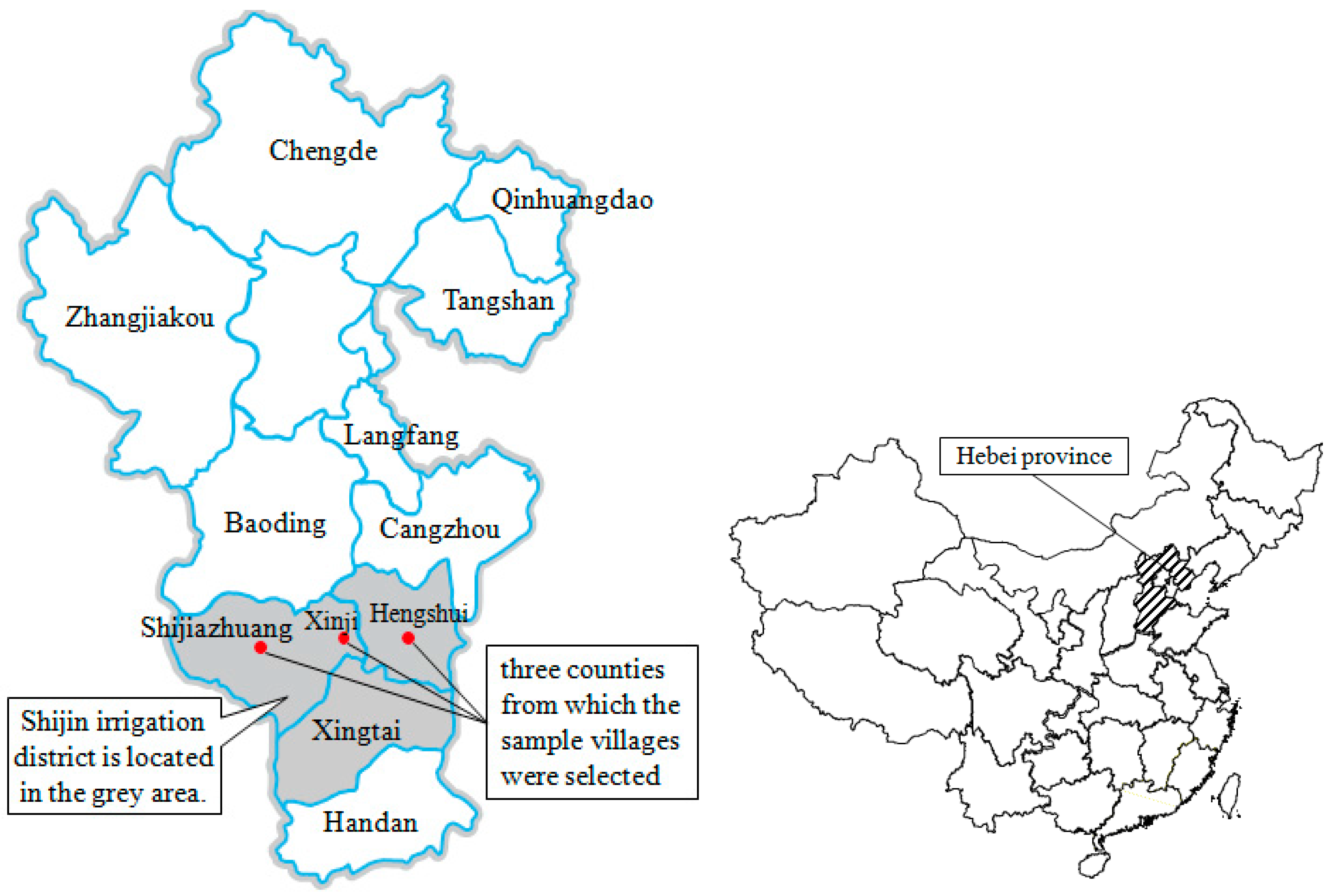
The analysis was based on the cross-sectional dataset collected by the author and collaborators in August 2015 in Hebei Province (
Figure 1) in North China. Hebei Province located in 39°18′ N and 116°42′ E, with an area of 187,700 km
2. Hebei Province has a temperate monsoon climate with an average annual precipitation of about 484.5 mm. Wheat and maize are the two staple crops produced in a single-year rotation [
48]. On average, 86% of cultivated land is allocated to wheat between October and June, then 85% to corn from June to October. Wheat and corn production accounts for almost 90% of households’ land use. Both output and inputs are calculated as the total from wheat and corn production.
A stratified random sampling strategy was used to select counties with varying degrees of water scarcity in Shijin Irrigation District (ID), the largest ID in Hebei Province. Counties were first sorted according to estimates of water resources available per capita and divided into three equally sized groups (the most water-scarce, the least water-scarce and the middle group). Next, three counties in each of the three groups were chosen randomly, and three sample villages were randomly selected from a register of all villages in each county. Within each village, 10 households were randomly selected. In total, 27 villages and 270 farm households were surveyed. In each household, the decision maker for agricultural production activities, who was able to answer detailed questions about local off-farm employment and migration, was selected as the respondent. In our analysis, three groups of households were dropped due to missing data. The first group includes 27 households that only use surface water. Information on the key variable, the volume of water used, is missing. This is because households pay for surface water on a per unit of land area. As a result, the volume of surface water used is not measured at the household level. The surface water using households only take up 10% of our sample. The exclusion of surface water using households is not likely to introduce sample selection bias. Surface water in general is much cheaper than groundwater. Because of the price differences, farmers in rural China almost invariantly prefer surface water if it is available. The availability of surface water depends on the presence of canals and available water supplies from the ID. Neither factor can be influenced by individual farmers. Therefore, the choice of using groundwater or surface water is largely exogenous in our analysis. The second group includes 12 households that have missing information on one or more variables. The third group includes four households that did not irrigate wheat at all. The final sample has 227 households.
Table 1 lists definitions of all variables used in the empirical analysis and reports summary statistics of variables used in this study. In our sample area, the average total household land holding is 7.63 mu (0.51 hectare). This is in line with the prevailing small-scale farm in China. The average land input in wheat and corn production is 12.46 mu. Using the formula in previous studies [
49,
50,
51], the total amount of groundwater pumped in this paper is calculated as: Q = T × 129.5741 × BHP/(DEP + (255.5998 × BHP
2)/(DEP
2 × DIA
4)) where Q is the volume of groundwater pumped in cubic meters, T represents total hours of pumping, BHP denotes the power of engine in horsepower, DEP is the depth of well in meters, and DIA is the diameter in inches of pipe used with pumps. Out of the 1746 m
3 groundwater used to irrigate wheat and corn, about 745 m
3 is applied to irrigate corn and 1001 m
3 applied to irrigate wheat. This is consistent with the fact that wheat relies more on irrigation than corn. About 82% of households have at least one member participating in off-farm employment. Among those, 14% participate only in local off-farm employment and 20% only in migration, while the majority of the households, about 48%, participate in both migration and local off-farm employment. Among the households with individuals engaged in migration, 45% of family laborers were migrant workers. Among the households with local off-farm employment, 52% of family laborers were involved in local off-farm work. Averaged across all households (with or without off-farm employment), the share of migrant workers in family laborers is 15% and the share of laborers working off-farm locally is 36%. This is consistent with the recent trend that local off-farm employment has surpassed migration to become the dominant off-farm activity in rural China.
The average share of elderly laborers in the households reaches nearly 38%, which reflects the typical structure of household laborers in rural China. With large shares of children and elderly as well as an increasing share of off-farm laborers, the share of agricultural laborers in farm households is on the decline. The average age of respondents is 54.13 years, which reflects the aging problem in China’s agricultural sector. Only 19% of the households have received extension services. The average well depth reaches 125 m. in the sample area. The well depth observed in the sample areas is deeper than most areas in North China, which is among the most water scarce area worldwide.
5. Results and Discussion
Table 2 reports the estimated production function parameters βs in Equation (1). The parameters βs are not directly estimated. Instead Equation (4) is estimated. Then the estimates of βs are recovered from the estimated αs based their relationship described in the Empirical specification section. Since Equations (4) and (5) are estimated simultaneously in one step, the estimation results of Equation (4) when Equation (5) is estimated with OLS are different from those when Equation (5) is estimated with 2SLS. Therefore, two sets of estimates of βs are reported in
Table 2. The first set (column 1) is obtained using the results of the joint estimation of Equations (4) and (5) using the method of MLE. The second set (column 2) is obtained using the results of the joint estimation of Equations (4) and (5) with the method of MLE and 2SLS is applied to Equation (5).
The coefficients for input factors (
Table 2, column (2)) show that land is the most important factor significantly influencing wheat and corn production, with an elasticity of 2.38. This means that, ceteris paribus, a one percent increase in land leads to 2.38% increase of output value. The importance of increasing land input has been supported in literature [
52]. Though not significant, the negative sign of fertilizer and material indicates the slight overuse of chemical inputs in agricultural production in China. This is consistent with most findings in previous studies [
53,
54]. With a
p-value of 0.52, we fail to reject the null hypotheses of constant returns to scale.
Table 3 summarizes estimated IWE for households with and without individuals engaged in off-farm employment activities. The average IWE for the entire sample is found to be 88.31%, which means that, at the observed levels of other inputs and the same production technology, the same level of output can be produced with 11.69% less irrigation water. Households with individuals engaged in migration or local off-farm employment (87.60%) have slightly lower average IWE than households without members engaged in off-farm employment (91.62%). The difference, however, is not statistically significant.
The findings in
Table 3 do not necessarily mean there is no difference in IWEs between the two groups of households. First, the descriptive statistics reported in
Table 3 do not control for any factors that may influence IWE. So it may not reveal the true relationship between off-farm employment and IWE. For example, if households with larger farm are more likely to engage in off-farm employment and farmers with smaller farms tend to enjoy higher technical efficiency, then we may observe a spurious negative relationship between off-farm employment and technical efficiency. Second,
Table 3 reveals that although the average IWE is smaller for that of the group of households with off-farm activities (87.6 versus 91.6), the standard error is larger for this group (19.9 versus 9.23). The larger variation means that the IWEs of households with off-farm activities are less clustered around the mean. Some have low IWEs while others have high IWEs. In other words, some households with off-farm activities have higher IWEs than households without any off-farm activities while other households have lower IWEs. Third, the simple descriptive analysis in
Table 3 cannot identify a nonlinear relationship between the total off-farm employment and IWE, which is very likely to lead to the observation of no statistical difference between the mean IWEs. For instance, if IWE increases with the total off-farm employment up to a certain point, then decreases as the total off-farm employment increases. This nonlinear relationship makes it possible that in
Table 4, when only the mean IWEs are compared, no statistical difference is observed.
In the following analysis, we have distinguished between two different types of off-farm employment: the share of laborer migrated and the share of local off-farm laborers. Because there is no strong one-to-one correspondence between total off-farm employment (as denoted in
Table 3) and the share of laborer migrated, or between total off-farm employment and the share of laborers working off-farm locally, the estimated coefficients on these variables are not expected to have the same signs or similar levels of statistical significance.
The sample area shows a high IWE relative to others. Karagiannis et al. estimated IWE as 47.20% [
9] and Chebil et al. found that as 61.25% [
10]. However, both studies examined IWE in vegetable production. In the study of Tang et al., the average IWE is 35% [
13]. The higher estimated IWE in our study are likely explained by differences between the study areas in the first place. The main off-farm activities in the study area in China are jobs in the manufacturing, construction and service industries, where salaries are relatively low. The sample area in the study of Karagiannis et al. is selected from Crete in Greece where the high annual off-farm income mostly comes from tourism. This means farmers in Greece are less focused on agricultural production.
Another difference is that Hebei is among the most water scarce areas in China and worldwide. In Hebei, irrigation water efficiency is generally higher in more water-scarce sub-areas. Tanner and Sinclair argued that the economic view of efficient water use is most easily recognized in arid-region irrigated agriculture where water is scarce [
55]. Karaba et al. pointed out that water scarcity results in stresses like drought and salinity, which may promote adoption of drought-resistant crops, which in turn results in higher IWE [
56]. Tang and Folmer observed a positive and statistically significant relationship between the degree of water scarcity as perceived by farmers and the level of IWE [
57].
Additionally, in the study of Tang et al. wheat irrigation is mainly organized by irrigation districts and relies on surface water [
13], while our study examines households’ groundwater IWE. The 2006 National Irrigation Water Use Efficiency Measure and Analysis Report shows that IWE is relatively high in areas irrigated by groundwater (about 0.60) and lower in surface water areas (lower than 0.40) [
58]. This is probably because less seepage loss occurs during conveyance in the groundwater irrigated area [
16]. Farmers’ plots are located closer to wells than to the branch canals that supply surface water, so the conveyance distance is shorter for groundwater. In addition, surface plastic pipes are often used to deliver groundwater to the fields while surface water often flows through mud canals.
Table 4 reports coefficients for the determinants of IWE (
Table 4, columns (2) and (4)). Notably, the negative sign of coefficients indicates a positive relationship between IWE and variables under consideration, since the one-step approach measures the factors influencing technical inefficiency. The results provide evidence to support the income effect on IWE. Other things held constant, a one percentage point increase in the share of family laborers working locally leads to IWE increase by 13.98%. One reason is that remittance from off-farm income alleviates the credit constraints experienced by rural households. Off-farm income can be used to finance irrigation investment and to get better access to irrigation technologies, which helps farmers obtain higher irrigation efficiency. Our result is in line with previous findings that time spent on farming has significantly negative impact on IWE and there is a significant positive relationship between income and IWE [
13].
Among the characteristics of household laborers and decision makers, the share of elderly laborers is the only factor negatively and significantly affecting households’ IWE. Households with a higher share of elderly laborers have lower IWE. Households with a large share of elderly laborers have less available laborers on farm, as well as less laborers on irrigation water management. This finding is in line with previous studies [
28]. None of the coefficients for characteristics of decision-makers is significant.
The robust positive relationship between total land area and inefficiency indicates that smaller farms are more efficient in irrigation water use. This finding is consistent with previous studies [
1,
9,
12,
59]. A positive coefficient for fragmentation indicates that fragmentation can be a barrier to increasing IWE. It is also found that households have higher IWE if the soil quality of their land is considered as good. Studies have shown that IWE is higher in surface-irrigated areas with appropriate soils and low with shallow soils [
60].
Well depth is used as a proxy for water price in our model. The robust negative sign indicates that pricing water higher helps to improve IWE. Similar arguments have been made in previous studies. Cummings and Nercissiantz have proposed that water pricing can be used as a means for improving IWE [
61]. In addition, Huang et al. have found, that reforming water pricing can induce water-savings, but the price of water needs to be raised to a relatively high level [
62].
Two significant negative coefficients of the interaction terms are found between the number of furrows and the share of laborers migrated, and between the number of furrows and the share of laborers working off-farm locally. This supports the existence of heterogeneous effects of local off-farm employment on IWE across households with different furrow irrigation levels. In addition, the number of furrows, as a moderator, adjusts the effect of off-farm employment on IWE. The more furrows households have in fields, the greater the positive effect of local off-farm employment on IWE. In other words, effects of local off-farm employment on improved IWE can be moderated and enhanced in households at higher levels of furrow irrigation. Raine and Bakker reported that significant higher IWE can be achieved through better management of furrow irrigation [
63]. As more laborers in households participate in off-farm employment, less labor is available in furrow irrigation. While preparing land for furrow irrigation is a one-time per season task, it remains time consuming. Nonetheless, once furrows are dug, less pumping is needed to achieve the same rate of irrigation application in the field, because seepage losses are reduced with more furrows. Therefore, despite the initial labor requirement, furrow irrigation saves the total amount of irrigation labor needed for the whole irrigation season.


