Article

Groundwater Hydraulics in Increased Spring Discharge following Earthquakes: Some Applications and Considerations

by
Eugenio Sanz Pérez
,
Juan Carlos Mosquera-Feijóo
*,
Joaquín Sanz de Ojeda
and
Pablo Rosas Rodrigo
ETSI Caminos, Canales y Puertos, Universidad Politécnica de Madrid, 28040 Madrid, Spain
*
Author to whom correspondence should be addressed.
Water 2024, 16(4), 520; https://doi.org/10.3390/w16040520
Submission received: 28 December 2023 / Revised: 31 January 2024 / Accepted: 2 February 2024 / Published: 6 February 2024
(This article belongs to the Special Issue How Earthquakes Affect Groundwater)

Abstract

:
Earthquakes often entail alterations in the groundwater flow regime, in the phreatic level, surges and losses of springs, and the discharge in brooks. A variety of theoretical approaches attempt to elucidate the post-earthquake effects on spring discharge. This study adopts a conceptual approach, primarily presenting diverse methods to estimate water released by earthquakes involving calculations of discharge surpluses in springs. This study delves into refined techniques rooted in groundwater hydraulics, displaying applications of analytical and simulation methodologies to quantify earthquake-induced groundwater discharge in springs. This research investigates springs as natural indicators and applies mathematical precipitation–runoff models, particularly the CREC model, to simulate hydrographs in post-earthquake scenarios. We apply analytical procedures or mathematical simulation techniques employed in groundwater hydraulics for natural aquifer recharge calculations. Firstly, we briefly describe the methods based on the analysis of depletion curves of hydrographs in spring discharge. Additionally, specific mathematical rainfall–runoff models used to simulate hydrographs of karstic springs, along with derived analytical approximations, are adapted for this scenario. These hydraulic calculations involve the depletion coefficient and hydrodynamic volumes of aquifers, parameters that reveal certain aspects of the relation between groundwater and earthquakes. Three main features are: (a) Acknowledging faults as the primary geological structures in transmitting pore pressures due to earthquakes. Thus, for large and deep faults, which connect the ground surface with the Earth’s crust bottom—where earthquakes trigger—the depletion coefficient, α, usually reaches high values (α = 0.1 days−1). Therefore, these faults become more sensitive to pore pressure than other lithologies. (b) Elucidating the mechanisms of permeability enhancement caused by earthquakes. (c) Highlighting the substantial volumes in motion within the Earth’s interior, which, for instance, could constitute a significant source for the origin of mineral deposits. Mathematical calculations enable the determination of the volume of mobilized water that can be discharged by gravity in each earthquake. This, along with its recurrence, justifies the substantial mineralization volumes.

1. Introduction

As is known, one of the most common hydrogeological effects induced by earthquakes is the persistent increase in spring and stream discharge connected to aquifers, as well as the rise in piezometric levels [1,2]. These post-seismic flow increases can impact extensive areas and last for days, months, or even years. However, post-earthquake increases in water levels in wells are not universal phenomena. There may also be prolonged drops in water levels [3,4].
The most pronounced spring discharge increase after earthquakes is typical for gas-saturated groundwater. A possible reason for this phenomenon is the transition of dissolved gas to a free state under the influence of seismic waves on the feeding aquifer system. Such a possible mechanism for a sharp increase in spring water flows after earthquakes has also been reported [5].
While extensively documented, the origins of these changes remain a subject of debate. These observed phenomena result from the interaction between hydrogeological processes and the mechanical and tectonic properties of the Earth’s crust in response to seismic deformation [6]. Hence, they provide insight into the interaction among water cycle, tectonics, and crust properties. An earthquake induces changes in static and dynamic stresses in the crust, which decrease differently with distance.
The ultimate origin of these phenomena involves various mechanisms related to static and dynamic stresses [6,7], permeability changes [3,7,8,9,10,11], and sediment consolidation [9,11,12,13]. However, common hydraulic explanations draw on the ease or sensitivity of an aquifer to the increase in piezometric or hydraulic head potential due to the earthquake, manifesting in the rise in groundwater levels (groundwater level changes). This rise may result in the emergence of new springs or an increase in the flow of existing springs and water streams. This hydraulic explanation is directly related to diverse hydrogeological parameters of the aquifer, including diffusivity (hydraulic diffusivity) and the aquifer-specific storage coefficient, among others.
Sanz de Ojeda et al. [14], reviewed the hydrogeological parameters that significantly influence the hydrological impact of earthquakes and developed a theoretical analytical model. They proposed the depletion coefficient as the primary sensitivity parameter for persistent water level changes and alterations in springs in general.
Our conceptual research provides insights into the application of groundwater hydraulics to increased spring discharges induced by earthquakes. Hydraulic calculations involve the depletion coefficient and hydrodynamic volumes of aquifers, revealing aspects of the interplay between groundwater and seismic activity.
Specifically, the pursued objectives in this research are as follows:
  • Proposing various methods for estimating volumes and excess groundwater mobilized by earthquakes in springs. Analytical procedures or mathematical simulation methods used in groundwater hydraulics for calculating natural aquifer recharge are applied.
  • Explaining some of the potential mechanisms of increase and decrease in aquifer discharges induced by earthquakes based on the results of applying spring hydraulics, and clarifying the mechanisms of increased permeability during earthquakes, drawing attention to the large volumes moving internally, which could be a significant source of the origin of mineral deposits, for instance.
  • Recognizing faults as the primary geological structures in transmitting pore pressures due to earthquakes.

2. Materials and Methods

To estimate the excess spring discharge caused by earthquakes, we present procedures based on the analysis of depletion curves in spring hydrographs. We also adapt mathematical rainfall–runoff models used in simulating karstic spring hydrographs, along with analytical approximations derived from these models. We emphasize the potential and validity of these methods for studying this subject, such as predicting how a spring behaves during a seismic event.

2.1. Terminology and Background

2.1.1. The Depletion Coefficient of a Spring

Natural groundwater discharges on continents may occur through springs, which are localized outflows with appreciable flow rates, often associated with contacts between lithologies of varying permeability. Alternatively, discharges can occur diffusely along water streams hydraulically connected to the aquifer’s water table.
The discharge rate of a spring from an aquifer with constant-level outflow under conditions unaffected by pumping or recharge, for example, is defined by the depletion curve, which can be calculated using an exponential-type equation:
Q t   L 3 T 1 = Q 0 e α t   ,
where Q t is the discharge at time t , Q 0 is the initial discharge at the beginning of the recession or depletion curve ( t 0 = 0 ), and the depletion coefficient is denoted by α (established by Boussinesq in 1877) [15]. The expression for the depletion coefficient, α , is given by [16]:
α   T 1 = 2 ( K   b ) S L 2
This equation implies that the depletion coefficient not only depends on the hydrogeological parameters of the aquifer, K   L T 1 (hydraulic conductivity) and S (storage coefficient), but also on the aquifer geometric properties: L is the length from the center of gravity of the aquifer to the discharge point and b is the average saturated thickness of the aquifer. The aquifer transmissivity T is given by T = K b .
The definition of α in this equation could be described as the mathematical integration of L along the x direction of the flow transect through its thickness b and length from the initial discharge point to the center of the aquifer.
To obtain the volume of groundwater stored in an aquifer above the spring (hydrodynamic volume or reserves) at the beginning of the recession period t 0 = 0 , it is sufficient to integrate expression (1) from 0 to infinity:
V t 0 = t 0 Q t d t = t 0 Q 0 e α t d t = Q t 0 α     V t 0 = Q t 0 α   .
From Equation (3), it can be seen that α has the dimension of t 1 . Its value can be determined from Equation (1) through the depletion phase hydrograph as follows:
ln Q t   = ln Q 0 α t   α = ln Q 0 ln Q t   t   .
If a sufficiently filled aquifer is conceptualized as multiple flow layers with different depletion coefficients α 1 ,   α 2 ,   α 3 ,   α n , the expression for Q t would be
Q t = Q 01   e α 1 t + Q 02   e α 2 t +   Q 0 n   e α n t ,
Water circulation within the saturated zone can be highly complex, involving interactions with other potential porous or fractured aquifers, the coexistence of interconnected or non-interconnected fissures and conduits with different hydrodynamic properties, etc. [17]. These conditions depend on the position of the piezometric surface. It is generally accepted that when the latter is shallow at the beginning of discharge in an unconfined flow regime (after an earthquake, for example), drainage of all conduits and fissures, both large and small, occur. Undoubtedly, wider fissures drain more rapidly (higher slope α 1 ). However, after a certain point, their flow becomes negligible compared with that of smaller cracks, which often represent a larger volume of water but with a slower rate (lower slope α 2 ).

2.1.2. Theory of Seismic-Origin Discharge during Spring Recession

An earthquake originating from a nearby or distant source can cause a sudden increase or decrease in hydraulic head in an aquifer. From a hydraulic perspective, these are considered external actions on the aquifer. Unlike natural meteoric-origin recharge, other factors like precipitation and air temperature do not influence this recharge. Instead, it is triggered by a single, very rapid tectonic event. Also, clearly establishing the lower recharge area of the aquifer is uncertain, as it depends primarily on vertical hydraulic conductivity and, in any case, on the greater or lesser hydraulic connection with source zones where positive or negative pore pressures occur, even if these are shallow.
In the case of a pore pressure increase, regardless of the potential mechanisms that may cause it, there is a groundwater bottom-up flow ( B ), rapidly raising the piezometric level and increasing the hydrodynamic volume to V . Here, V is the sum of the hydrodynamic volumes before the earthquake ( V 1 ) and those caused by the seismic event ( V 2 ), so that V = V 1 + V 2 (see Figure 1). After the earthquake, and until the previous equilibrium is restored through the depressurization of the system, this increase in stored volume can be drained in two ways: through either an outward flow via new or existing springs or a downward flow ( B ). The latter becomes evident, for example, through the water level decrease measured by piezometers in aquifers without outlets. This can occur due to depressurization effects, as part of the general tendency to restore tectonic equilibrium. After restoring equilibrium, a residual volume might remain undrained, evident through a positive change in the water level.
Both piezometric levels and discharge increases are two ways of measuring the same phenomenon, which is a rapid pressure pulse initially and slow depressurization afterward. This becomes evident since the recession curve is similar for either well levels or spring discharges. This indicates that the depressurization mechanism is the same.
Depending on the initial situation and the increase in piezometric level due to the earthquake, the geological setting of the aquifer, and the site’s topography, we can consider three common cases (see Figure 2):
  • If the piezometric level was already at the surface, then the earthquake will result in an increase in the discharge of existing springs and streams. The excess water due to the earthquake emerges to the surface and can be measured using flow gauging stations.
  • If the piezometric level did not reach the surface, but its increase due to the earthquake gives rise to new springs and streams, only a portion of the excess water due to the earthquake can be measured at a flow gauging station; the rest can be observed through the water level decrease.
  • If the increase in the piezometric level due to the earthquake does not reach the surface, the excess water can only be observed through changes in the water level but cannot be quantified in terms of discharge.
The analysis in this work primarily builds on the first and second cases. Hence, the analysis specifically addresses variations in spring flows, not piezometric levels in wells.
Earthquakes initially produce a filling of the aquifers with water and, consequently, a large increase in the flow of the springs; then, as the aquifer empties, water flow and discharge decrease over time (see Figure 2). As mentioned earlier, the aquifer can naturally operate with a discharge reflected in hydrographs that respond to mathematical functions of a single exponential (1) or a sum of several exponentials (5). Generally, it is a single exponential, but there could be a scenario where, during the period of increased flow due to the earthquake, the spring is discharging with two or more exponentials. However, we will disregard it in our analysis since it is a rare situation.

3. Results and Discussion

3.1. Spring Depletion Coefficient Due to the Earthquake

The case illustrated in 
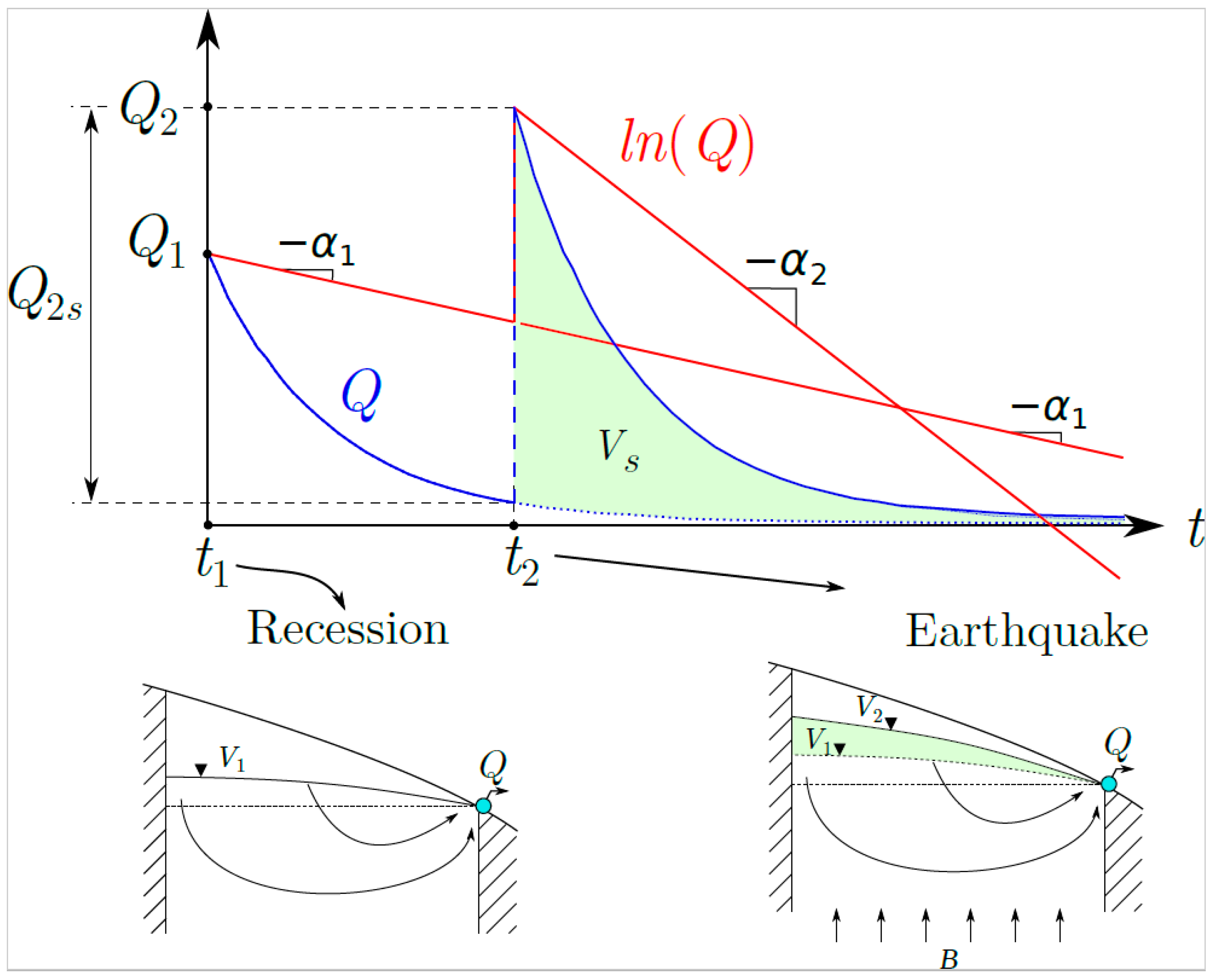
Figure 2a involves two depletion coefficients. This is reflected in the final resulting discharge curve: the one representing the aquifer’s discharge as if there had been no seismic effect, and the exponential curve due to the earthquake (α1 is the recession coefficient of the discharge curve before the seismic event, and α2 is the depletion coefficient due to the earthquake). These two depletion coefficients have been observed in actual cases in both well levels and spring discharge hydrographs, e.g., for the 1989 Loma Prieta earthquake [6], for the 1999 Chi-Chi earthquake [16,18,19], and for the Mw8.8 Maule 2010 earthquake in Chile [20]. Figure 3 depicts such a response, which, although it seems the most logical, does not occur in all the cases consulted.
A sketch of this hydrograph, neglecting aquifer inertias, is the composite recession curve shown in Figure 3. In this case, in a semi-logarithmic diagram, the hydrograph would consist of two straight lines, and the expression for the depletion curve would be:
Q = Q 1   e α 1 t + Q 2 s   e α 2 t     ,   t > t 2   .
In this expression, Q 1 stands for the initial discharge at the beginning of the spring or stream depletion curve before the earthquake, α 1 is the pre-earthquake depletion coefficient of the spring discharge curve, Q 2 s is the increase in discharge mobilized by the earthquake, and α 2 is the coefficient of its depletion curve. However, it might also occur that only an increase in discharge could be observed, but with the same depletion curve characteristic of the spring before the earthquake ( α 2 = α 1 ).
Some springs have revealed that after the earthquake-induced discharge increase, the aquifer depletes with its initial, interseismic α value, behaving hydraulically as usual. This fact has been documented for the 1989 Mw6.9 Loma Prieta earthquake [21] and the 1999 Chi-Chi earthquake [18,19,22]. Hence, Wang and Manga [11,12] deduced that the increased permeability mechanism could not explain the increased spring discharge due to earthquakes, given that the depletion coefficient of a spring before and after an earthquake does not vary.
However, this does not seem to be the case, as a sensitivity analysis of the diverse variables involved in this coefficient, according to Equation (2), seems to show that significant increases in permeability involve imperceptible variations in the depletion coefficient. Thus, according to Equation (2), of the four variables influencing the depletion coefficient ( K ,   b ,   S , and L ), we can consider b and L as fixed for each specific aquifer. S depends on the aquifer type (unconfined, semi-confined, or confined), and its variation concerning K is much smaller according to Darcy’s law. In other words, small increments of S imply significant increases in K . Additionally, K appears multiplied by two. This analysis only seeks to envisage the influence of S on K , rather than performing a sensitivity analysis of S . The reason is to demonstrate that a large variation in K , being the factor that furthest affects the depletion coefficient, hardly varies.
For example, in the Vozmediano Spring (Spain), with an average discharge of 1100 L/s, if the permeability of the entire aquifer varies from K = 1.1 m/day to K = 1.2 m/day, the depletion coefficient would change from α = 0.0033 to α = 0.0036 [22,23,24,25,26]. We would need to increase an order of magnitude ( K = 2 m/day) for the coefficient to vary relatively significantly ( α = 0.006 ). We can then verify that significant changes in aquifer permeability are masked within the margins of measurement errors of spring discharge gauging. The changes in slope on the recession lines are so small that they are imperceptible at the hydrograph drawing level.
This does not imply that there cannot be a very significant increase in permeability occurring at great depths, near the rupture zone, but its influence on the average permeability of the entire aquifer will be small if the aquifer draining the spring is large (parameter L in Equation (2)). However, if we restrict ourselves to faults, we do believe that vertical permeability can be substantially improved over geological timescales.
The ratio between the size of the aquifer and that of the fault ruptured by the earthquake is a relevant factor. In an aquifer with tens or hundreds of km2, the size of a crossing fault can be small. Even if the entire fault slips, it has little impact on the average permeability. However, if the fault itself embodies the aquifer and is surrounded by an impermeable ground, its permeability variation can become high. When faults constitute the aquifers, spring discharges are rather low. Large flow springs are usually related to massive aquifers entailing large recharge surface, although the faults associated with them become the outlet conduits. Mathematical models are valuable tools to quantify these responses in each case; otherwise, it is elusive beforehand.
The geological mechanisms that can increase vertical permeability would not only be those produced by the hydraulic fracture of the at-depth earthquake but also the increase in the fault slip, caused by friction failure between the contacting blocks, and the increase in the fault opening, cleaning the fault plane, among others.

3.2. Calculation of Post-Seismic Excess Discharge and the Mobilized Volume of Water Due to Earthquakes

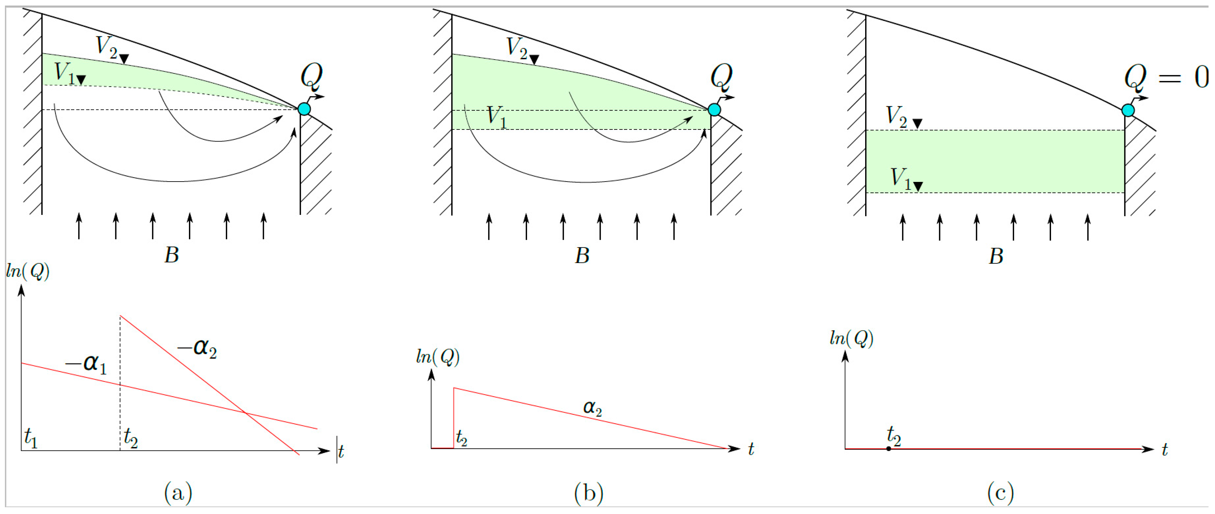
Not all water mobilized by an earthquake can be quantified as post-seismic excess discharge, as it does not always come to the surface. This occurs when piezometric levels only rise but later return to lower levels and reach equilibrium. Therefore, the estimation of excess discharge measured in springs and streams will be a minimum of the water mobilized by earthquakes.
In the case of new springs and streams (see Figure 2c), after the initial abrupt increase, there will be a descending branch in the hydrograph with slope α 1 , as in the previous case, until the new spring dries up at t 1 , after which only the piezometric level descent due to depressurization or downward flow will operate.
In case 2-D, only levels are available, and the effect operating in the piezometric level descent is the downward flow, with the manifestation of a single descending branch with slope α 2 . If tools were available to convert elevations into discharge (mathematical models, for example), discharge hydrographs could be obtained, and excess volumes due to earthquakes could be calculated.

3.2.1. Estimation of the Volume Mobilized by an Earthquake Using the Hydrograph of a Spring

The volume of water discharged by the earthquake ( V s ) is the increase in hydrodynamic volume of the aquifer, which, from the hydrograph, can be calculated as the difference between the volume discharged by the spring after the earthquake and what it would have discharged if the earthquake had not occurred:
V S   L 3 = V 2 V 1 = t 2 Q 1 e α 1 t + Q 2 s e α 2 t d t t 2 Q 1 e α 1 t d t = t 2 Q 2 s e α 2 t d t ,
where Q 1 is the spring discharge at the beginning of the recession and Q 2 s is the flow induced by the earthquake. A simple way to estimate this volume is
V S   L 3 = V 2 V 1 = V 2 Q 1 α 1 Q 2 α 2 Q 1 α 1   .
Expression (7) can be easily related to the colored region of Figure 3, i.e., V S . The previous graph corresponds only to the case in which the spring was flowing at the time of the earthquake occurrence. The possibilities with their respective graphs (see Figure 2) are as follows.

3.2.2. Analysis of Spring Hydrographs

Regardless of other methods for calculating recharge using piezometric variations or mathematical models, we will focus here on those that utilize the spring hydrograph. We will consider recharge as the excess discharge draining through a spring due to an earthquake. These methods are based on the analysis of hydrograph peaks: the surges that occur as a result of upward flow due to an earthquake and their subsequent decline when the seismic activity has ceased. In addition to the method proposed by Wang and Manga [12,13], we present below, as an example, the recession curve shifting method. Other similar methods can be found in Sanz Pérez [23,24,25,27]. The goal is not to exhaust the topic but to adapt and apply hydrogeological theory to earthquake scenarios to demonstrate the possibilities of these estimations.

3.2.3. The Recession Curve Shifting Method

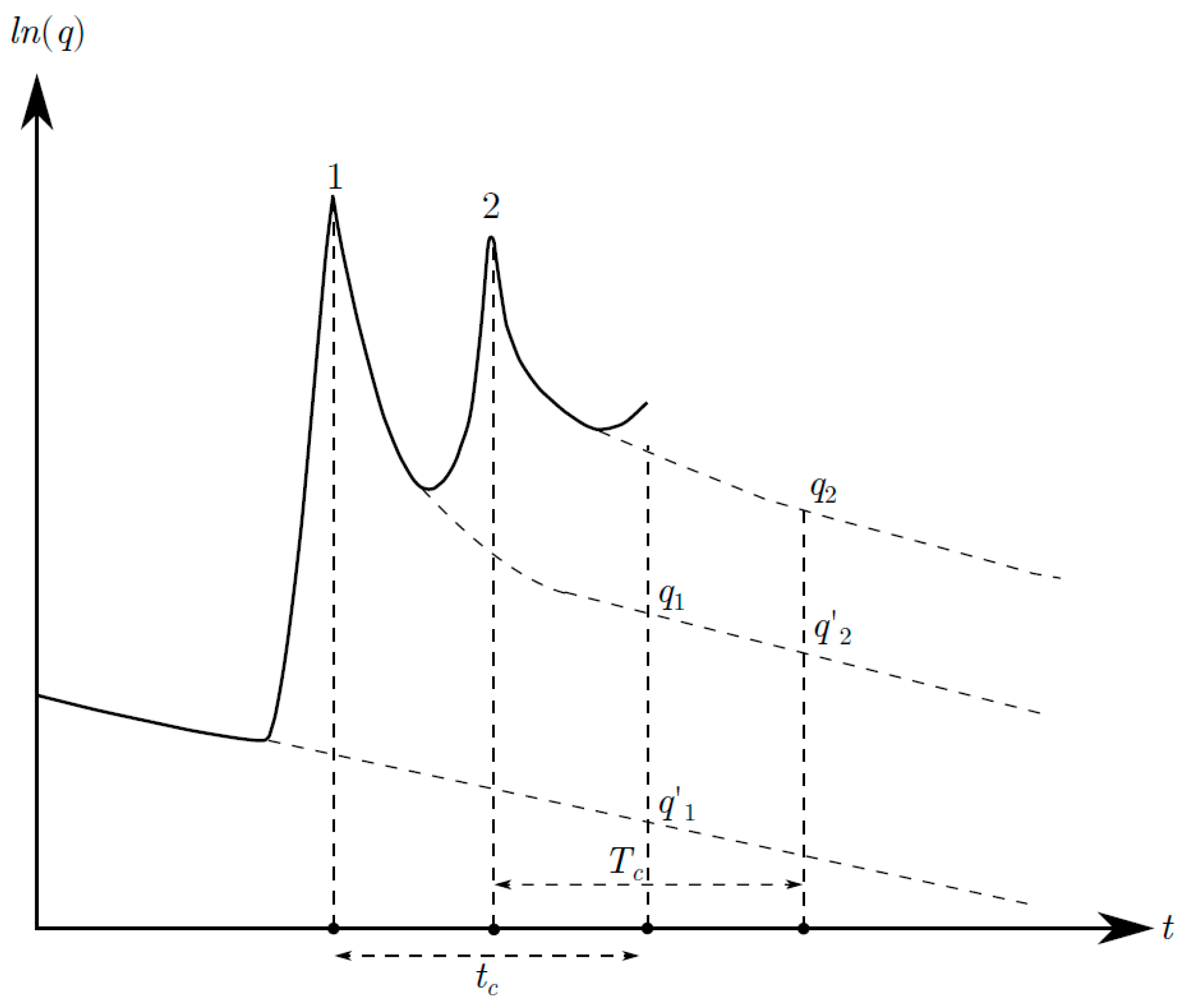
This method is based on raising the recession curve of the discharge ensuing from recharge induced by an earthquake from below. It includes the possibility of analyzing the inflow injections from various events, such as aftershocks, although the first event causes the most significant surge in the spring. If α is the depletion coefficient, which has been determined beforehand, it assumes that at the so-called “critical time” ( t e = L / 2 α ) from the end of the recharge, the spring acquires its base flow.
For each hydrograph peak, with semi-logarithmic representation (see Figure 1), estimate on the graph the descent curve of the peak until it becomes parallel to the recession line or, in other words, with slope α, at the “critical time.” At this moment, measure the flows q i from the recession line of the peak and q i from the previous recession.
Formulations by Glover [28] and Rorabaught [29], automated later by Rutledge and Daniel [30], show that the total potential groundwater recharge at a critical time after the flow peak is approximately equal to half the recharged water volume into the system. Therefore, for peaks 1 and 2 in Figure 4, the following recharges R j and R 2 would be obtained:
R j = 2 q 1 α q j α = 2 q 1 q j α ;       R 2 = 2 q 2 q j α   .

3.2.4. Rainfall–Runoff Mathematical Models

For the mathematical description of recharge and discharge transfer in the simulation of spring hydrographs and well levels, mainly aggregated models (uni- and multicellular models) have been employed, some of which are also called black-box models. A variety of authors have explained some of such models, e.g., [23,30,31,32].
A simple and effective model is the single-cell model, which considers the aquifer as a linear reservoir in which the volume of stored water above the outlet level relates to the discharge through a depletion coefficient, as expressed in Equation (4). Otherwise, multicellular models are suitable when the spring has several depletion coefficients.
In the encompassed multicellular models, for example, modeling is expressed exclusively under drained flow conditions, volumes, and recharges in each decomposition cell. Therefore, knowledge of piezometric level series is not required, as they do not intervene in the calculation. The quantification of evapotranspiration is not required, nor is the aquifer geometry and conditions at the borders; only the total surface of the aquifer and the precipitation and natural flow gauge series of the spring are necessary.
Both unicellular and multicellular models can be used to analyze the effect of pumping or recharge induced by an earthquake. These models are more suitable than finite difference or finite element ones for heterogeneous media. The reason is that these latter models require knowing the parameters of the aquifer distributed over its spatial domain, which is very difficult. On the contrary, all these aggregate or black-box models explained below build exclusively on the analysis of the spring hydrograph. These aggregate models suggest that the interpretation of attributing the slopes these pluricellular models may not be as complete, but they can simulate the hydrograph very well. Another question is whether we can draw direct geological conclusions. For example, different depletion coefficients with different slopes are not exclusively due to differences in hydraulic conductivity.
Some other valuable models, such as SIMERO [23,25,27] or CREC [29,31], are very appropriate for the research at hand. These models consider the aquifer as divided into three deposits distributed in series and representing three successive water stages, from precipitation to its outlet to the spring. In the first, a conventional hydraulic balance is operated, from which the water comes out to the unsaturated zone (second deposit) and saturated (third deposit), where the flow undergoes a delay and phase shift. SIMERO can assume a linear and invariant system, by specifying such condition in the last two layers, and therefore, the circulation of water is expressed by a convolution integral. In the CREC model, the deposit representing the unsaturated zone is responsible for the nonlinear drainage of the aquifer and the transfer of flow to the saturated zone, and in the latter, linear drainage occurs. From these models, flows, pressures, and volumes can be obtained.

3.2.5. Application to the Case of Seismic Alteration of a Spring

These precipitation–runoff models could simulate not only flow variations but also pressure variations, i.e., piezometric level variations. For this, a reasonable assumption is made, such as that recharge comes from bottom to top, passing directly to the saturated zone. In this way, the flow does not undergo the reduction in balance in the soil, such as rain-infiltrated water, nor the delay and phase shift of the following deposits of mathematical models. It is as if we recharged the aquifer by injecting water through a well into the saturated zone.
As an example, we present the simulation of an earthquake affecting the Fuentetoba Spring (Soria, Spain) [32,33,34,
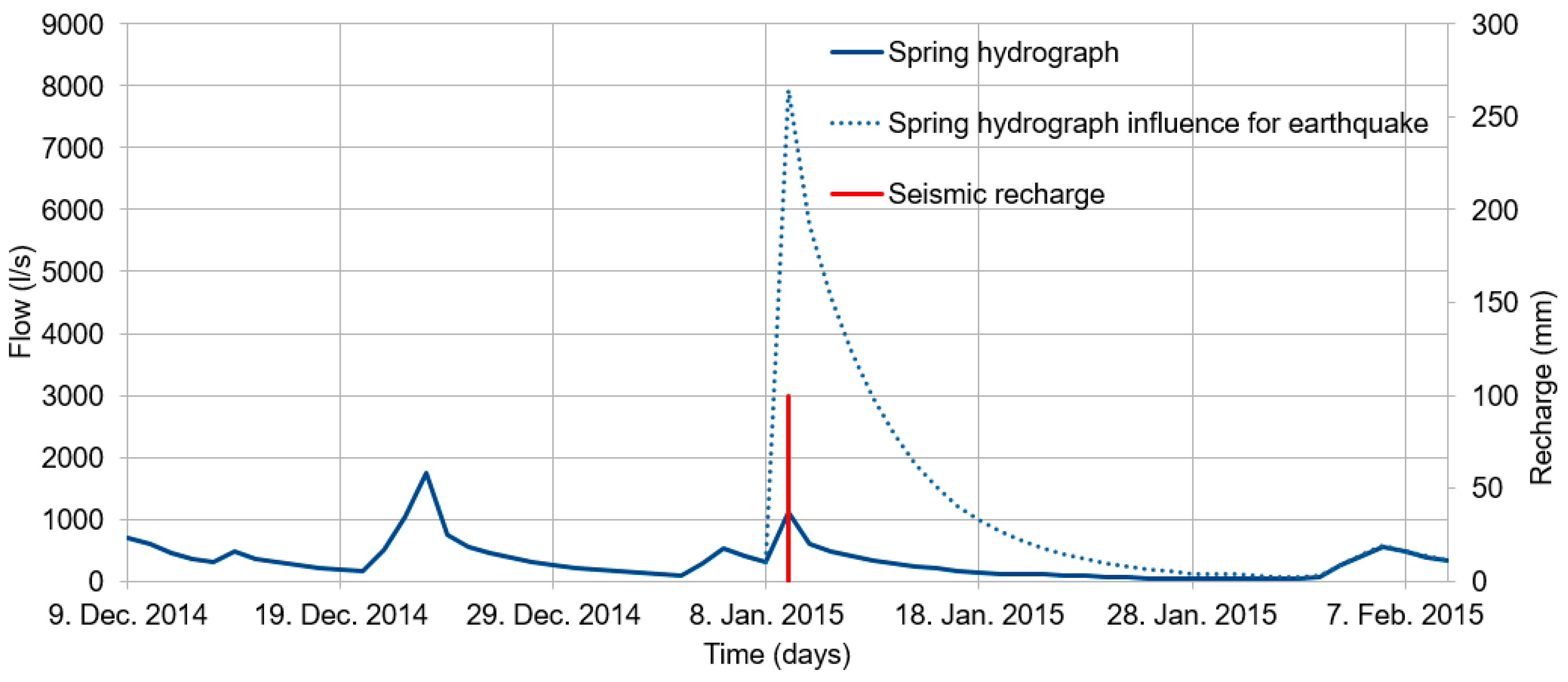
35]. This spring drains a karstic aquifer naturally, without exploitation wells, and the recharge comes only from rainfall. It has an average flow of 200 L/s, but a very variable regime, so that it has peaks of up to 7000 L/s, although it can also dry up. Its hydrograph has been simulated using the CREC model for 20 years, so it is very well calibrated. The first simulation of an earthquake involved injecting a recharge directly into the saturated zone during a rainless period and a dry spring, albeit with the water table at the natural drain outlet level of the spring. It could be assimilated somehow to the appearance of new springs due to the effect of an earthquake. The recharged flow was practically instantaneous (31 July 2011), and with a very large amount (100 mm spread throughout the aquifer). As shown in Figure 5, the reaction was immediate, with a vertical ascending branch in the hydrograph, and a spring-depletion-coefficient dependent recession that lasted more than a month, until it dried up again.
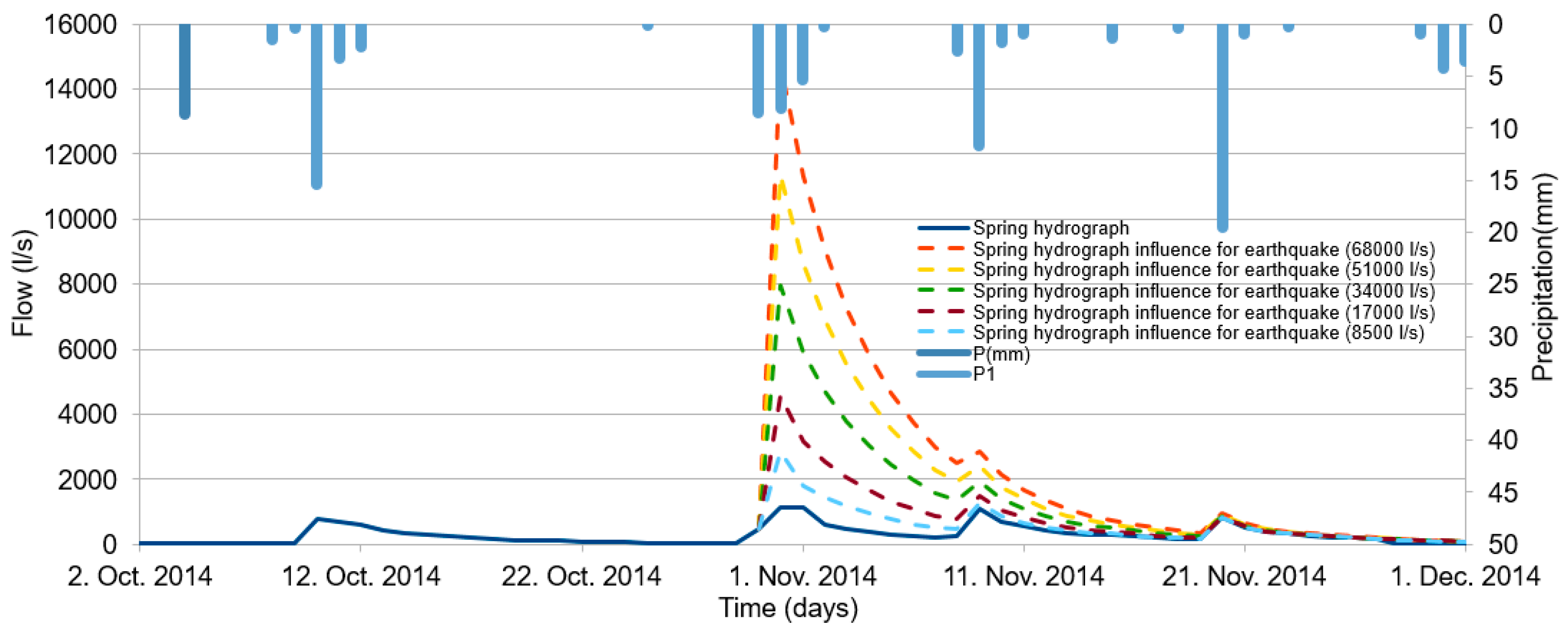
In the case of a spring that is active during seismic-induced recharge, Figure 6 presents the results of various simulations for the same Fuentetoba Spring. Different recharge values are considered for hypothetical earthquakes without aftershocks occurring on 30 October 2010. As expected, we observe the immediate effect of seismic recharge in all cases, and later, the aquifer emptying law is reflected according to its α, which prevails for seismic recharges with higher values. The separation in the hydrograph of the two effects, rainfall recharge and seismic recharge, is very clear. We highlight that the use of these models enables this differentiation even during intense rainfall events that could obscure a co-seismic increase. We also observe how the seismic effect persists for more than 15 days in all cases. The persistence time increases with seismic recharge, but it does not influence as much. It is assumed that aftershocks contribute to the persistence time.
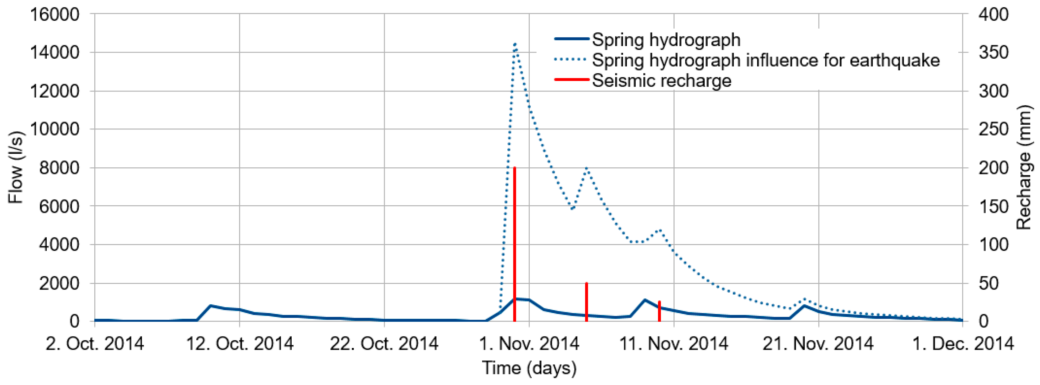
The last simulation assumed a 200 mm recharge, corresponding to the main earthquake, along with aftershocks 5 and 10 days later with 50 mm and 25 mm, respectively. Figure 7 depicts how the persistence time remains significantly longer, and the slopes vary based on the juxtaposition of events.

3.2.6. Effects of Seismic-Induced Recharge Actions Using Analytical Solutions Derived from Precipitation–Runoff Mathematical Models

After a spring has been previously simulated using a rainfall–runoff model, including its iterative formulas and once discretized, there are analytical solutions to calculate the effects on its flow from deep seismic-origin recharges. Pressure buildups (piezometric levels) can also be calculated. In these cases, the aquifer is considered homogeneous, and it is assumed that deep seismic-origin recharges are instantaneous and uniformly distributed along the aquifer or around its center of gravity. These induced actions consist of seismic-origin recharges, as mentioned (similar to artificial recharges in conventional hydrogeology), or effects of seismic pumping on the aquifer that lead to the decrease or drying up of springs (similar to groundwater pumping through wells in conventional hydrogeology). The mathematical treatment is analogous in both cases, but the sign of these recharges is changed.
For one of the most well-known mathematical models (SIMERO), these solutions are given in Sanz Pérez [23,25,27] and adapted to the case of fluid flow or pressure from an earthquake, summarized in the following iterative formula, where U ( I ) is the actual contribution of the spring, considering the effect of seismic recharges up to period I .
U I = U I + U R I   ,
where U ( I ) is the flow that the spring would have if there were no seismic-origin recharges in period I or the preceding ones, and U R I is the difference between the two aforementioned values, i.e., the increase in the historical flow of the spring due to all seismic-origin recharges made up until period I .
These formulas can be applied to the extreme case of a significant spring decrease and drying up due to earthquakes. It is a case opposite to those seen in this study but will serve to verify the possible mechanism that originates it. As an illustrative example, Vozmediano is a spring with an average flow of about 1100 L/s. This spring is located in the Iberian Mountain Range (Spain) and drains a large limestone aquifer over 1500 m thick with significant confinement. Its hydrodynamic volume at the average initial date of the depletion curves has been estimated as 25 hm3, with a flow rate of 870 L/s. Its hydrograph was simulated for 20 years using the SIMERO model [23,25,27], and presents an analysis of the effects on its flow from a possible artificial recharge made at the center of gravity of its aquifer.
According to Sanz et al. [32,33], this spring exhibits the same behavior during earthquakes: a sudden post-seismic decrease (never an increase) lasting several hours (no more than 24 h) and a rapid, progressive increase until the previous flow is restored. During recovery, the water comes out with white turbidity for no more than 24 h. This behavior repeats itself for strong or moderate earthquakes in both the far field—like the Lisbon earthquake of 1755, M (8.5–9)—and the near field (like the one on 3 September 1961 in Aguilar del Rio Alhama, La Rioja, Spain, M5). The flow modification depends on the felt intensity at the site, regardless of its magnitude and distance. In the nearby earthquake of Aguilar del Rio Alhama on 3 September 1961 (M5), the Vozmediano Spring, which had a flow rate of 780 L/s, gradually dried up within 20 min to an hour after the earthquake and two minutes after an aftershock. It remained completely dry for nine hours, leading to a lack of electrical production in the power plants until, also gradually, it recovered its previous flow. During the Lisbon earthquake of 1755, this spring dried up completely for approximately one day [34].
The consequences of these seismic events on the discharge of the Vozmediano Spring can be evaluated using Equation (7). This analysis helps confirm that achieving its desiccation would necessitate pumping a volume of water approximately equivalent to its hydrodynamic capacity within a single day, which is practically unattainable. To elucidate the potential desiccation mechanism of this spring, there is no need to invoke significant alterations in the hydraulic parameters of the aquifer. In this scenario, it appears evident that stress variations induced by earthquakes can lead to changes in elastic parameters and temporary deformations in the rock. Consequently, the storage coefficient, contingent upon the vertical compressibility coefficient of the aquifer and its substantial thickness in this instance, can undergo a temporary increment, enabling the retention of water that would otherwise discharge through the spring over a day.

3.3. Confirmation of Faults as Principal Pathways for Fluid Pressure Transmission Due to Earthquakes

While the fact that faults serve as preferential conduits for transmitting fluid pressure during seismic events is established, employing the depletion coefficient as a hydraulic parameter offers a quantifiable confirmation of this assertion. As demonstrated by Sanz de Ojeda et al. [14], the significance of faults as sensitive geological discontinuities for transmitting fluid pressure surpasses other lithologies during seismic events, particularly evident in the Lisbon earthquake of 1755, M (8.5–9).
Anticipating such behavior from faults seems reasonable, given their typical attributes as confined aquifers characterized by a very small storage coefficient ( S ) and a substantial length ( L 
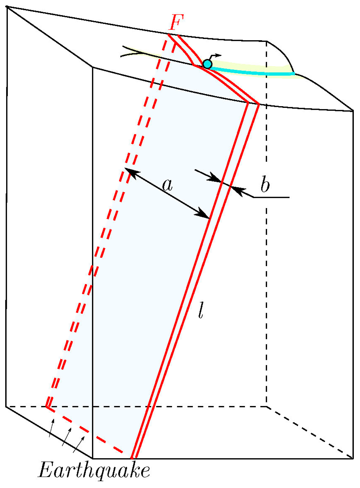
). Consider a fault F discharging through a spring (see Figure 8). This fault exhibits a small saturated thickness b (a few meters), a length L (hundreds of meters), and a subvertical (non-vertical) dip, ensuring that the aquifer in the fault zone becomes confined at shallow depths. Assigning standard values to the variables in Equation (2), and defining the depletion coefficient, such as k = 10 3   m / s for fractured zones (Hoek and Bray, 1981), S = 10 6 for confined aquifers like this one, and b = 10 m for major faults, gives us the following results:
  • If L = 1000 m ⇒ α = 2131.83 days−1.
  • If L = 5000 m ⇒ α = 85.27 days−1.
  • If L = 10,000 m ⇒ α = 21.31 days−1.
It is evident that all α values are greater than 0.1 days−1, and as the fault length L decreases, α (its hydraulic sensitivity to earthquakes) increases. While other factors ( k , b , S ) could be varied, these calculations suffice to verify that faults generally exhibit elevated α values. In conclusion, depletion coefficient (α) values corresponding to faults of considerable length, such as those connecting the Earth’s surface to the depths of the crust where earthquakes originate, tend to be high (α > 0.1 days−1). This heightened sensitivity to pore pressure renders faults more responsive than other lithologies.

3.4. On the Water Temperature Rise during an Earthquake

It has been observed that variations in the chemical composition and temperature of many springs that increase their flow due to earthquakes are not as substantial as might be expected initially (e.g., Rojstaczer and Wolf, in the 1989 Loma Prieta earthquake [
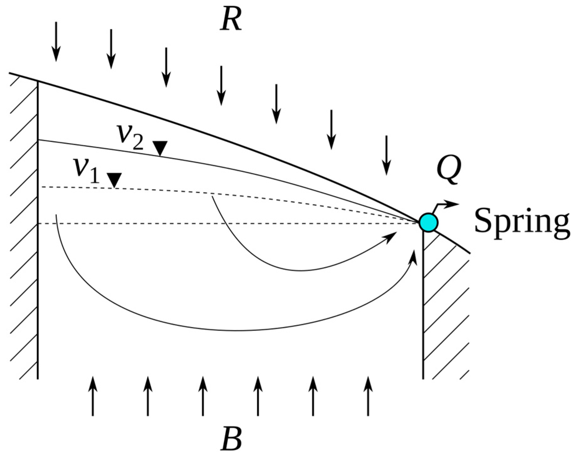
36]). However, as depicted in Figure 1 and Figure 2 and the equations derived here from a laminar Darcian regime, everything indicates a piston-type flow, where the fault rupture acts as a fluid pressure pump pushing groundwater upwards, with minimal mixing with the lower part. Despite this, the uplift eventually results in an increase in piezometric levels or surface spring flows. In other words, the water emerging originates from the upper part, which is similar in composition and temperature to that exiting the spring.
As the regime is laminar, the actual velocity is V r   L T 1 = K . i / m e , where K is hydraulic conductivity, i is the hydraulic gradient (the modification of i is crucial in the case of an earthquake), and m e is the effective porosity. For an earthquake at a depth of 5 km, for instance, a velocity of 5 km/day (5.78 cm/s) would be required for water to reach the surface in accordance with the observed rapid increase in hydrographs. However, even assuming this velocity, and with values for the dynamic viscosity of water at 100 °C and a fault width of 2 mm, for example, the Reynolds number would exceed the laminar regime. For greater depths, necessary velocities would demand turbulent regimes.
In summary, the bottom-up piston flow model and the Darcian laminar regime seem to explain why the water increment in springs after an earthquake does not significantly raise its temperature or alter its chemical composition.

3.5. Groundwaters Mobilized by Earthquakes and the Origin of Hydrothermal Mineral Deposits

As known, structural evidence indicating that the mineralization of hydrothermal deposits was synchronous with ancient host faults led many researchers to propose the connection between episodes of hydrothermal precipitation and increased seismic ruptures when those faults were active. The presence of fluids at high temperatures and high mineralization in the upper half of the seismogenic continental crust, the generation of permeability associated with rupture, and mineral precipitation due to sudden pressure reductions or fluid mixing at specific structural sites all indicate the significant role played by seismic pumping flow. This not only explains many deep hydrothermal deposits but also shallower deposits like those of the Mississippi Valley (ore type), whose source of mineralized thermal water is attributed to seismic origins associated with specific faults. The works of Sibson et al. are crucial in this regard [37,38]. However, this is not yet well-quantified. The application of groundwater hydraulics and mathematical models can shed light on the subject. For instance, estimating the hydrodynamic volumes mobilized by an earthquake over geological history is fundamental to understanding the mineralizing potential and capacity that seismic pumping can produce. This section only aims to initiate the topic.
Direct evidence of fluid involvement with earthquakes comes from post-seismic discharges near active faults. In the Chi-Chi earthquake alone, over 2 km3 of groundwater expelled through some streams was estimated [18,19,22]. One must consider that the water mobilized by an earthquake can surpass that expelled by springs and watercourses hydraulically connected to aquifers, as not all water can be drained by gravity to the exterior. As seen in Section 3.2.1, the water mobilized above the drainage level, which can be consistently drained through a spring activated by an earthquake, can be calculated in its hydrograph by the difference in hydrodynamic volumes before and after the earthquake. For instance, for a spring with a flow rate of 100 L/s and a constant depletion coefficient of α = 0.0033 days−1 that increases to 500 L/s due to an earthquake, the volume of water mobilized and drainable by gravity, calculated by the formula V = Q / α , would increase from 2.6 hm3 to 13.09 hm3, which is five times more. The time “ t ” it would take for this spring to return to 100 L/s without recharge would be determined by the equation:
t = ln Q 0 ln Q t α   ,
where Q 0 = 500 L/s (0.5 m3/s) and Q t = 100 L/s (0.1 m3/s), resulting in t = 487 days. The volume evacuated during this period would be 8.4 hm3.
The recurrence intervals between successive main earthquakes typically range from one decade to many thousands of years, depending on the fault’s activity level. Consider, for instance, an active fault with a return period of 500 years mobilizing 1 km3 in each event; this would be equivalent to a continuous flow of approximately 63 L/s over those 500 years. Moreover, a significant portion of the mobilized water expelled externally is likely to be from the upper part. Therefore, the hot and mineralized water is not renewed but rather stirred near the fault. This water fractures the rock, increases its porosity, mineralizes, and, in turn, refills it.

4. Conclusions

This work mainly aims to apply a part of conventional underground spring hydraulics to evaluate the increase in spring discharges induced by earthquakes.
As regards methodology, this article provides various techniques for estimating the volumes released externally and calculating seismic-origin recharge. For the calculation of this recharge, hydrograph analysis, mathematical rainfall–runoff models, and analytical functions derived from these are employed. Our findings confirm that mathematical models are particularly interesting as, once a spring is simulated under natural conditions before an earthquake, we can analyze and distinguish the earthquake’s effect on flow hydrographs or pressures (water levels in piezometers), or predict a spring’s behavior during seismic action. The rainfall during the post-seismic increase is considered in the simulated hydrograph and cannot obscure the induced earthquake flow response.
On the other hand, the analysis of the depletion coefficient recognizes faults as major geological structures in transmitting pore pressures due to earthquakes. It appears that this coefficient cannot be used as a tool to identify permeability changes during earthquakes. Finally, it emphasizes the large volumes of water moving within the crust, which could be a significant source of the origin of mineral deposits, for example.
Given that earthquakes and water interact through changes in both stress and the physical properties of rocks, understanding the origin of hydrological responses can provide valuable insights into hydrogeological and tectonic processes at spatial and temporal scales that would otherwise be challenging to study. Additionally, there is still much to learn about the interactions between water and earthquakes, with numerous unresolved issues. This research aims to give a step ahead in this regard.

Author Contributions

Conceptualization, E.S.P. and J.S.d.O.; methodology, E.S.P. and J.S.d.O.; software, P.R.R.; validation, E.S.P., J.C.M.-F. and P.R.R.; formal analysis, E.S.P. and J.S.d.O.; investigation, E.S.P., J.C.M.-F. and P.R.R.; resources, E.S.P., J.S.d.O. and J.C.M.-F.; data curation, E.S.P., J.S.d.O. and P.R.R.; writing—original draft preparation, E.S.P. and J.C.M.-F.; writing—review and editing, E.S.P., J.C.M.-F. and J.S.d.O.; visualization, E.S.P., J.C.M.-F. and J.S.d.O.; supervision, E.S.P. and J.C.M.-F.; project administration, E.S.P.; funding acquisition, E.S.P. All authors have read and agreed to the published version of the manuscript.

Funding

This research received no external funding.

Data Availability Statement

The data presented in this study are available from the authors upon request.

Acknowledgments

The authors gratefully thank the anonymous reviewers for their constructive criticism.

Conflicts of Interest

The authors declare no conflicts of interest.

Nomenclature

B L 3 T 1 upward flow due to earthquake-induced increased pore pressure
b   L average saturated thickness of the aquifer
i   hydraulic gradient
K   L T 1 hydraulic conductivity
L   L length from the center of gravity of the aquifer to the discharge point
m e % effective porosity
Q   L 3 T 1 flow rate
Q t   L 3 T 1 discharge at time t
Q 0   L 3 T 1 initial discharge, i.e., at the beginning of the depletion curve ( t 0 = 0 )
Q 1   L 3 T 1 spring or stream discharge at t 1 , i.e., the beginning of the recession, before the earthquake
Q 2   L 3 T 1 spring discharge at the moment of the earthquake
Q 2 s   L 3 T 1 increase in discharge induced by the earthquake at time t 2
R   L 3 T 1 natural meteoric-origin recharge
R j   L 3 T 1 recharges from other sources
S   T 1 aquifer storage coefficient
T   L 2 T 1 aquifer transmissivity
U I   L 3 T 1 actual contribution of the spring, considering the effect of seismic recharges up to period I
U I   L 3 T 1 flow that the spring would have if there were no seismic-origin recharges in period I or the preceding ones
U R I   L 3 T 1 increase in the historical flow of the spring due to all seismic-origin recharges made up until period I
V 1   L 3 hydrodynamic volume before the earthquake
V 2   L 3 hydrodynamic volume caused by the earthquake
V r   L T 1 actual velocity
V s   L 3 volume of water discharged by the earthquake
α   T 1 depletion coefficient
α 1 ,   α 2 ,   α 3 ,   α n depletion coefficients
α 1 pre-earthquake depletion coefficient of the spring discharge curve
α 2 coefficient of its depletion curve

References

  1. Nespoli, M.; Todesco, M.; Serpelloni, E.; Belardinelli, M.E.; Bonafede, M.; Marcaccio, M.; Gualandi, A. Modeling earthquake effects on groundwater levels: Evidences from the 2012 Emilia earthquake (Italy). Geofluids 2016, 16, 452–463. [Google Scholar] [CrossRef]
  2. Xiang, Y.; Peng, S. Changes in well water level and rock damage zones in a shallow aquifer before and after local earthquakes. Hydrogeol. J. 2023, 31, 1937–1951. [Google Scholar] [CrossRef]
  3. Liao, X.; Wang, G.; Shi, Z. Sustained Changes in Well Water Levels Following a Large Earthquake: Possible Evidence of Permeability Decreases in a Shallow Groundwater System. Geophys. Res. Lett. 2021, 48, e2020GL090232. [Google Scholar] [CrossRef]
  4. Kopylova, G.; Boldina, S. Seismo-Hydrogeodynamic Effects in Groundwater Pressure Changes: A Case Study of the YuZ-5 Well on the Kamchatka Peninsula. Water 2023, 15, 2174. [Google Scholar] [CrossRef]
  5. Kopylova, G.; Boldina, S. Hydrogeological earthquake precursors: A case study from the Kamchatka peninsula. Front. Earth Sci. 2020, 8, 576017. [Google Scholar] [CrossRef]
  6. Muir Wood, R.; King, G.C.P. Hydrological signatures of earthquake strain. J. Geophys. Res. 1993, 98, 22035–22068. [Google Scholar] [CrossRef]
  7. Wakita, H. Water wells as possible indicators of tectonic strain. Science 1975, 189, 553–555. [Google Scholar] [CrossRef]
  8. Jónsson, S.; Segall, P.; Pedersen, R.; Björnsson, G. Post-earthquake ground movements correlated to pore-pressure transients. Nature 2003, 424, 179–183. [Google Scholar] [CrossRef]
  9. Montgomery, D.R.; Manga, M. Streamflow and water well responses to earthquakes. Science 2003, 300, 2047–2049. [Google Scholar] [CrossRef] [PubMed]
  10. Elkhoury, J.E.; Brodsky, E.E.; Agnew, D.C. Seismic waves increase permeability. Nature 2006, 441, 1135–1138. [Google Scholar] [CrossRef] [PubMed]
  11. Di Matteo, L.; Dragoni, W.; Azzaro, S.; Pauselli, C.; Porreca, M.; Bellina, G.; Cardaci, W. Effects of earthquakes on the discharge of groundwater systems: The case of the 2016 seismic sequence in the Central Apennines, Italy. J. Hydrol. 2020, 583, 124509. [Google Scholar] [CrossRef]
  12. Wang, C.Y.; Manga, M. Earthquakes and Water. In Lecture Notes in Earth Sciences; Springer: Berlin/Heidelberg, Germany, 2010; Volume 114, ISBN 978-3-642-00809-2. Available online: https://www.springer.com/series/772 (accessed on 8 September 2023).
  13. Wang, C.Y.; Manga, M. Water and Earthquakes. In Lecture Notes in Earth System Sciences (Open Access); Springer: Berlin/Heidelberg, Germany, 2021; ISBN 978-3-030-64307-2. [Google Scholar] [CrossRef]
  14. Sanz de Ojeda, A.; Alhama, I.; Sanz, E. Aquifer sensitivity to earthquakes: The 1755 Lisbon earthquake. J. Geophys. Res. Solid Earth 2019, 124, 8844–8866. [Google Scholar] [CrossRef]
  15. Boussinesq, J. Essai sur la théorie des eaux courantes. Mémoires présentés par divers savants à l’Académie des Sciences France. Impr. Natl. 1877, 23, 252–260. [Google Scholar]
  16. Chia, Y.P.; Wang, Y.S.; Wu, H.P.; Huang, C.J.; Liu, C.W.; Lin, M.L.; Jeng, F.S. Changes of ground water level in response to the Chi-Chi earthquake. In International Workshop on Annual Commemoration of Chi-Chi Earthquake; National Center for Research on Earthquake Engineering: Taipei, China, 2000; pp. 317–328. Available online: http://ntur.lib.ntu.edu.tw/handle/246246/134812 (accessed on 8 September 2023).
  17. Liu, B.; Yan, G.; Ma, Y.; Scheuermann, A. Measurement of In-Situ Flow Rate in Borehole by Heat Pulse Flowmeter: Field-Case Study and Reflection. Geosciences 2023, 13, 146. [Google Scholar] [CrossRef]
  18. Wang, C.-Y.; Wang, C.-H.; Kuo, C.-H. Temporal change in groundwater level following the 1999 (Mw = 7.5) Chi-Chi earthquake, Taiwan. Geofluids 2004, 4, 210–220. [Google Scholar] [CrossRef]
  19. Chia, Y.; Wang, Y.S.; Chiu, J.J.; Liu, C.W. Changes of groundwater level due to the 1999 Chi-Chi earthquake in the Choshui River alluvial fan in Taiwan. Bull. Seismol. Soc. Am. 2001, 91, 1062–1068. [Google Scholar] [CrossRef]
  20. Mohr, C.H.; Manga, M.; Wang, C.Y.; Korup, O. Regional changes in streamflow after a megathrust earthquake. Earth Planet Sci. Lett. 2017, 458, 418–428. [Google Scholar] [CrossRef]
  21. Manga, M. Origin of postseismic streamflow changes inferred from base flow recession and magnitude-distance relation. Geophys. Res. Lett. 2001, 28, 2133–2136. [Google Scholar] [CrossRef]
  22. Wang, C.Y.; Wang, C.H.; Manga, M. Coseismic release of water from mountains: Evidence from the 1999 (Mw = 7.5) Chi-Chi, Taiwan, earthquake. Geology 2004, 32, 769–772. [Google Scholar] [CrossRef]
  23. Sanz Pérez, E. Application and simplification of the SIMERO model for the Vozmediano Spring (Spain). Hydrol. Sci. J. 1996, 42, 763–779. [Google Scholar] [CrossRef]
  24. Sanz Pérez, E. Estimation of Basin Wide Recharge Rates Using Spring Flow, Precipitation, and Temperature Data. Groundwater 1997, 35, 1058–1065. [Google Scholar] [CrossRef]
  25. Sanz Pérez, E. Management of an aquifer with artificial recharge using water balance. Hydrol. Sci. J. 1997, 42, 909–918. [Google Scholar] [CrossRef]
  26. Sanz Pérez, E. Simulación de la recarga artificial de un acuífero en su manantial. Aplicación al manantial de Vozmediano. Estud. Geológicos 1997, 53, 17–23. [Google Scholar] [CrossRef]
  27. Sanz Pérez, E. Simulation of Spring Management with Quasi Aggregated Model. J. Hydrol. Eng. 1999, 4, 77–79. [Google Scholar] [CrossRef]
  28. Glover, R.E. Ground-Water Movement. U.S. Bureau of Reclamation Engineering Monograph Series 31; United States of the Department Interior: Washington, DC, USA, 1964; pp. 31–34. [Google Scholar]
  29. Rorabaugh, M.I. Estimating changes in bank storage and ground-water contribution to streamflow. Int. Assoc. Sci. Hydrology. Publ. 1964, 63, 432–441. [Google Scholar]
  30. Rutledge, A.T.; Daniel, C.C. Testing and automated method to estimate ground-water recgarge from streamflow records. Ground Water 1994, 32, 180–189. [Google Scholar] [CrossRef]
  31. Guilbot, A. Modélisation des Ecoulements d’un Aquifer Karstique (Liasons Pluie–Débit). Aplication aux Bassins de Saugras et du Lez. Ph.D. Thesis, Université des Sciences et Techniques du Languedoc, Montpellier, France, 1975. [Google Scholar]
  32. Estrela, T.; Sahuquillo, A. Modeling the Response of a Karstic Spring at Arteta Aquifer in Spain. Ground Water 1997, 35, 18–24. [Google Scholar] [CrossRef]
  33. Rosas, P.; Sanz, E.; Menéndez-Pidal, I. Hidrogeología del Karst de Pico Frentes (Cordillera Ibérica, España). Estud. Geológicos 2016, 72, 1–21. [Google Scholar] [CrossRef]
  34. Sanz, E.; Menéndez-Pidal, I.; Escavy, J.I.; Sanz de Ojeda, J. Hydrogeological Changes Along a Fault Zone Caused by Earthquakes in the Moncayo Massif (Iberian Chain, Spain). Sustainability 2020, 12, 9034. [Google Scholar] [CrossRef]
  35. Sanz, E.; Rosas, R.; Menéndez-Pidal, I.; Sanz de Ojeda, J. Management and Conservation Strategies for Fuentetoba Springs (Spain). Sustainability 2020, 12, 10131. [Google Scholar] [CrossRef]
  36. Rojstaczer, S.; Wolf, S. Permeability changes associated with large earthquakes: An example from Loma Prieta, California, 10/17/89 earthquake. Geology 1992, 20, 211–214. [Google Scholar] [CrossRef]
  37. Sibson, R.H.; Moore, J.M.M.; Rankin, A.H. Seismic pumping hydrothermal fluid transport mechanism. J. Geol. Soc. Lond. 1975, 131, 635–659. [Google Scholar] [CrossRef]
  38. Sibson, R.H. Faulting and Fluid Flow. In Short Course on Fluids in Tectonically Active Regime of the Continental Crust; Nesbitt, B.E., Ed.; Mineralogical Association of Canada: Vancouver, BC, Canada, 1990; pp. 93–132. [Google Scholar]
Figure 1. Conceptual model of an unconfined aquifer under the effect of an earthquake, discharging with flow rate Q through a previously existing spring. Diverse flow components include natural meteoric-origin recharge R , upward flow B due to earthquake-induced increased pore pressure, hydrodynamic volume V 1 before the earthquake, and hydrodynamic volume V 2 caused by the earthquake.
Water 16 00520 g001
Figure 2. Diverse situations and responses of an unconfined aquifer to an earthquake. (a) The spring is in recession, and the earthquake produces an increasing discharge that decreases with a steeper depletion curve. (b) The earthquake causes a dry spring to emerge. (c) The earthquake causes an increase in the aquifer’s piezometric level, but the spring does not emerge.
Water 16 00520 g002
Figure 3. Hydrograph in natural and semi-logarithmic scale of a spring in an unconfined flow regime (recession) that undergoes, at time t 2 , the instantaneous effect (without inertia or delays) of deep (bottom-up) pumping B due to the action of an earthquake. The post-earthquake slope of the spring’s depletion curve is assumed larger than before the earthquake ( α 2 > α 1 ). For t 1 t t 2 the depletion curve follows the equation Q t = Q 1 e α 1 t . From t 2 onward, the discharge curve is expressed as Q t = Q 1 e α 1 t + Q 2 s e α 2 t . Q 1 is the spring discharge at the beginning of the recession t 1 , Q 2 s is the discharge induced by the earthquake at time t 2 , and Q 2 is the spring discharge at the moment of the earthquake: Q 2 = Q 2 s + Q t 2 = Q 2 s + Q 1 e α 1 t 2 .
Water 16 00520 g003
Figure 4. Displacement of the recession curve for seismic recharge estimation.
Water 16 00520 g004
Figure 5. Effect of simulating a hypothetical earthquake on a dry spring. It is worth mentioning the sudden response of Fuentetoba Spring to the earthquake input.
Water 16 00520 g005
Figure 6. Hydrographs from hypothetical earthquake simulations by considering diverse earthquake-induced recharge increment values for an operating spring during the event.
Water 16 00520 g006
Figure 7. Simulation of the resulting hydrograph from the increased flow due to excess recharge from the main seismic event (200 mm) and two aftershocks (50 mm and 25 mm).
Water 16 00520 g007
Figure 8. Fault parameters influencing the definition of its depletion coefficient from Equation (2).
Water 16 00520 g008
Disclaimer/Publisher’s Note: The statements, opinions and data contained in all publications are solely those of the individual author(s) and contributor(s) and not of MDPI and/or the editor(s). MDPI and/or the editor(s) disclaim responsibility for any injury to people or property resulting from any ideas, methods, instructions or products referred to in the content.

