
Appraisal of Land Cover and Climate Change Impacts on Water Resources: A Case Study of Mohmand Dam Catchment, Pakistan
 , ,
, ,  , ,
, ,  ,
,  and
and
Abstract
:1. Introduction
2. Study Area and Datasets
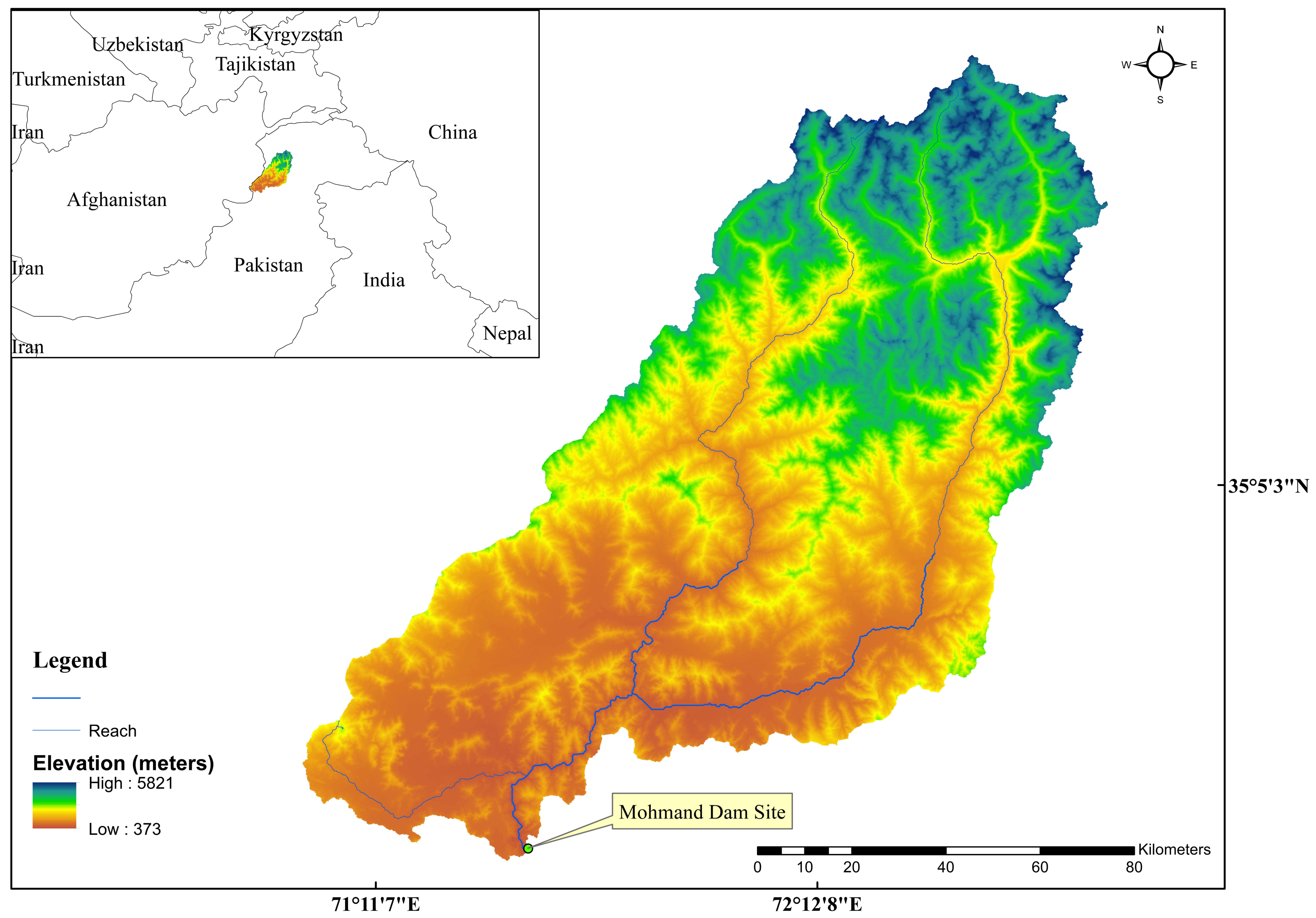
2.1. Study Area
2.2. Datasets
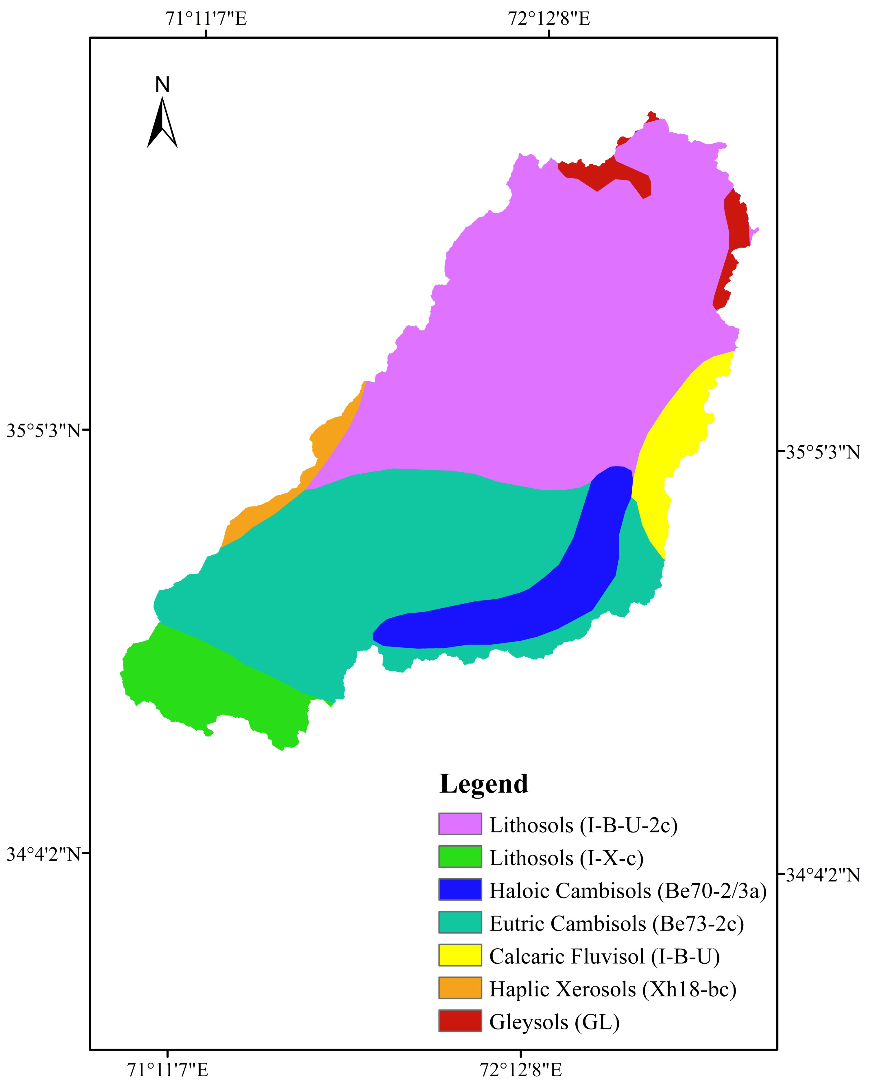
2.2.1. Soil Data
2.2.2. GCMs-Based Climate Data
2.2.3. Flow Data
3. Methodology
3.1. Statistical Downscaling
3.2. Description and Setup of the SWAT Model
3.3. Calibration and Validation of the SWAT Model
Model Performance Evaluation
3.4. Land Cover Scenarios and Validation of Land Cover Prediction
3.4.1. Markov Chain Analysis
3.4.2. CA–MARKOV
4. Results
4.1. Downscaling of Future Climate Data
4.1.1. Selection of the GCM
4.1.2. Selection of Bias Correction Techniques
4.2. Probable Changes in the Precipitation and Temperature
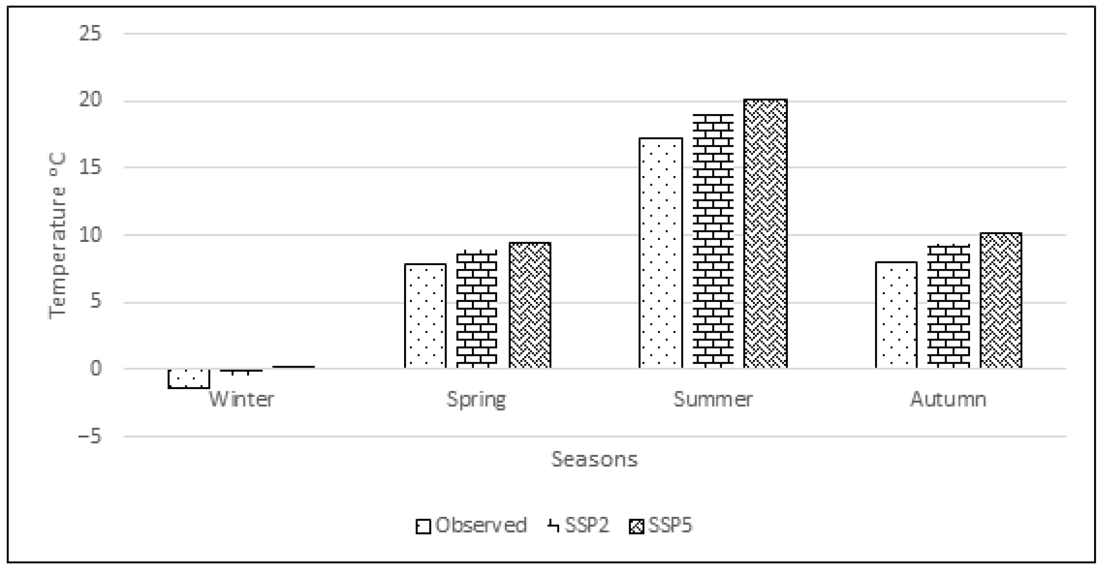
4.2.1. Projection of Mean Maximum Temperature
4.2.2. Projection of Mean Minimum Temperature
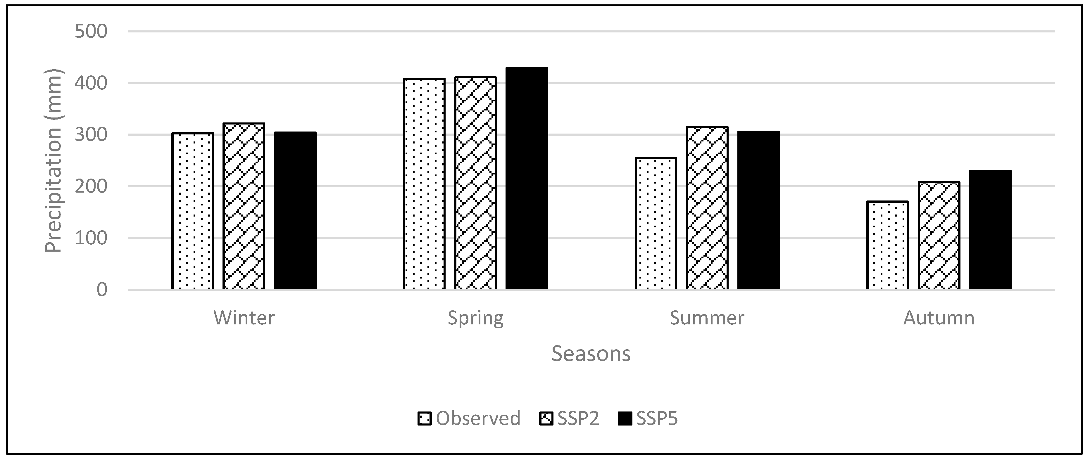
4.2.3. Projection of Precipitation
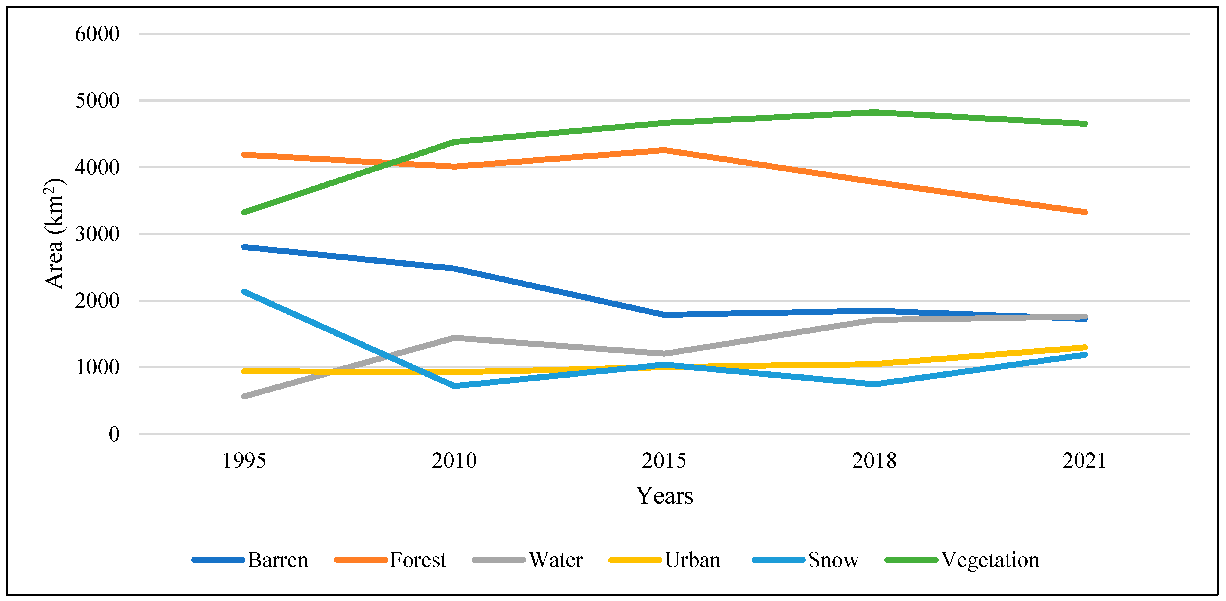
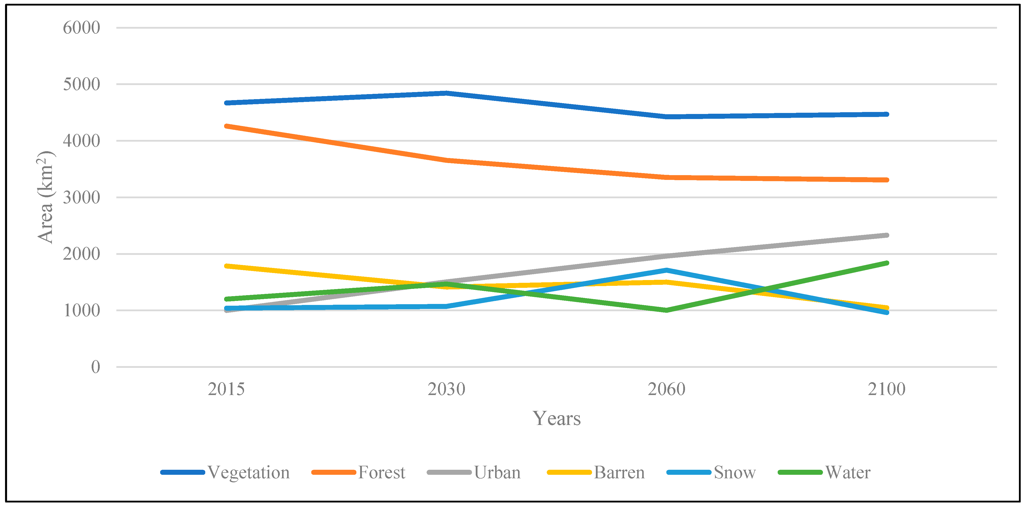
4.3. Land Cover Change Trends
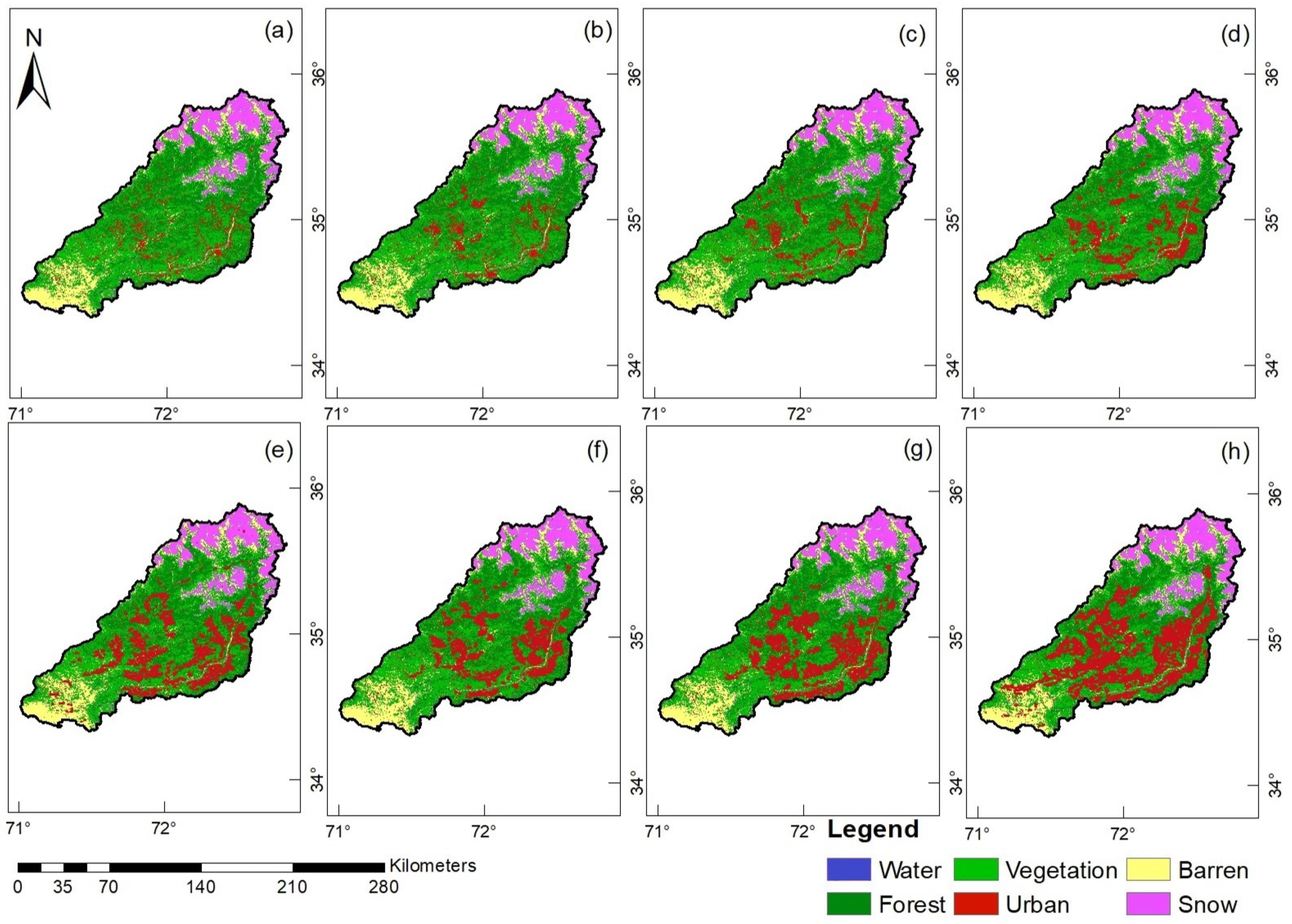
Future Land Cover Maps
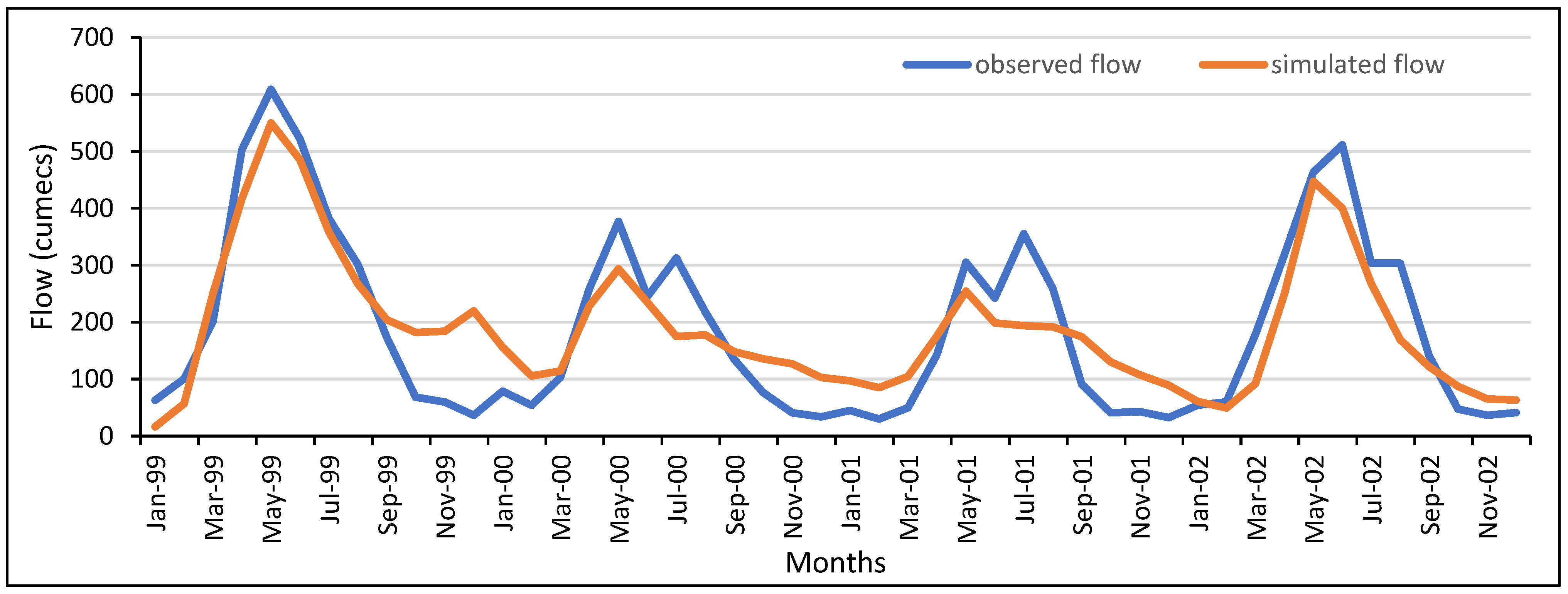
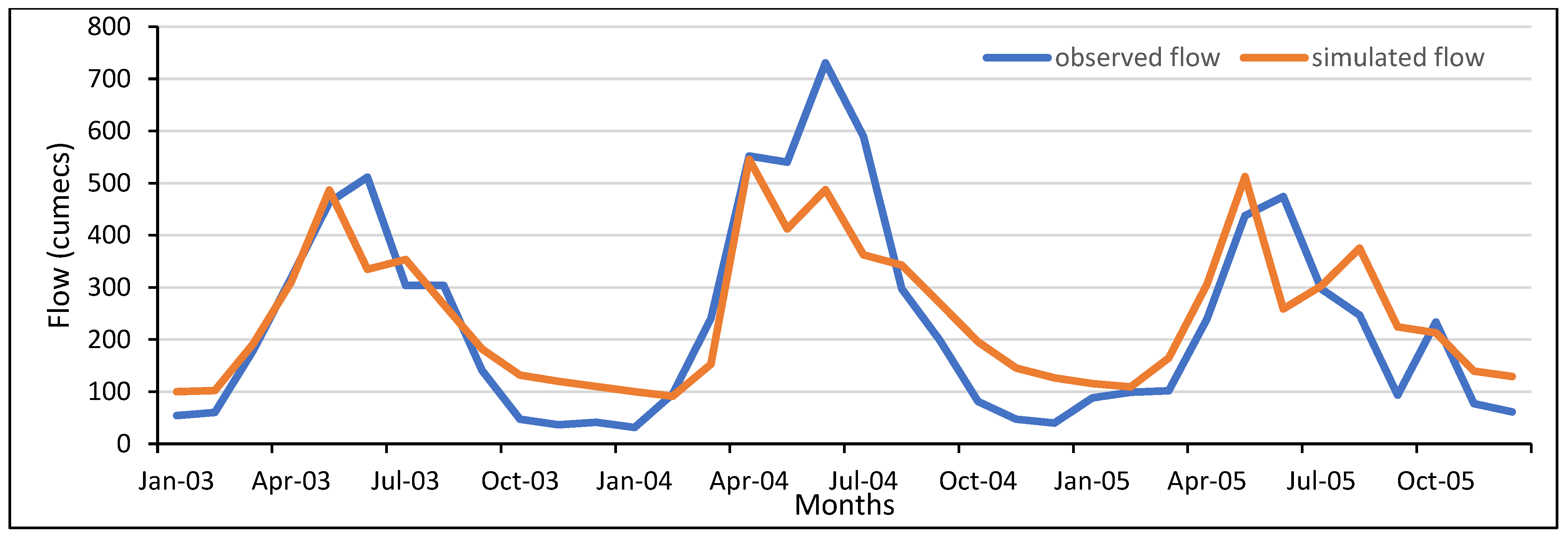
4.4. Calibration and Validation of the SWAT Model
4.5. Impact of Projected Climate on Flows
4.5.1. Scenario A: Climate Change Only
4.5.2. Scenario B: Climate and Land Cover Change
5. Discussion
6. Conclusions
- Compared to the baseline period (1990–2015), the annual maximum, minimum and mean temperature and precipitation increased consistently in the Mohmand Dam catchment in the future time horizon (2016–2100). The increased precipitation leads to increased streamflows in the future;
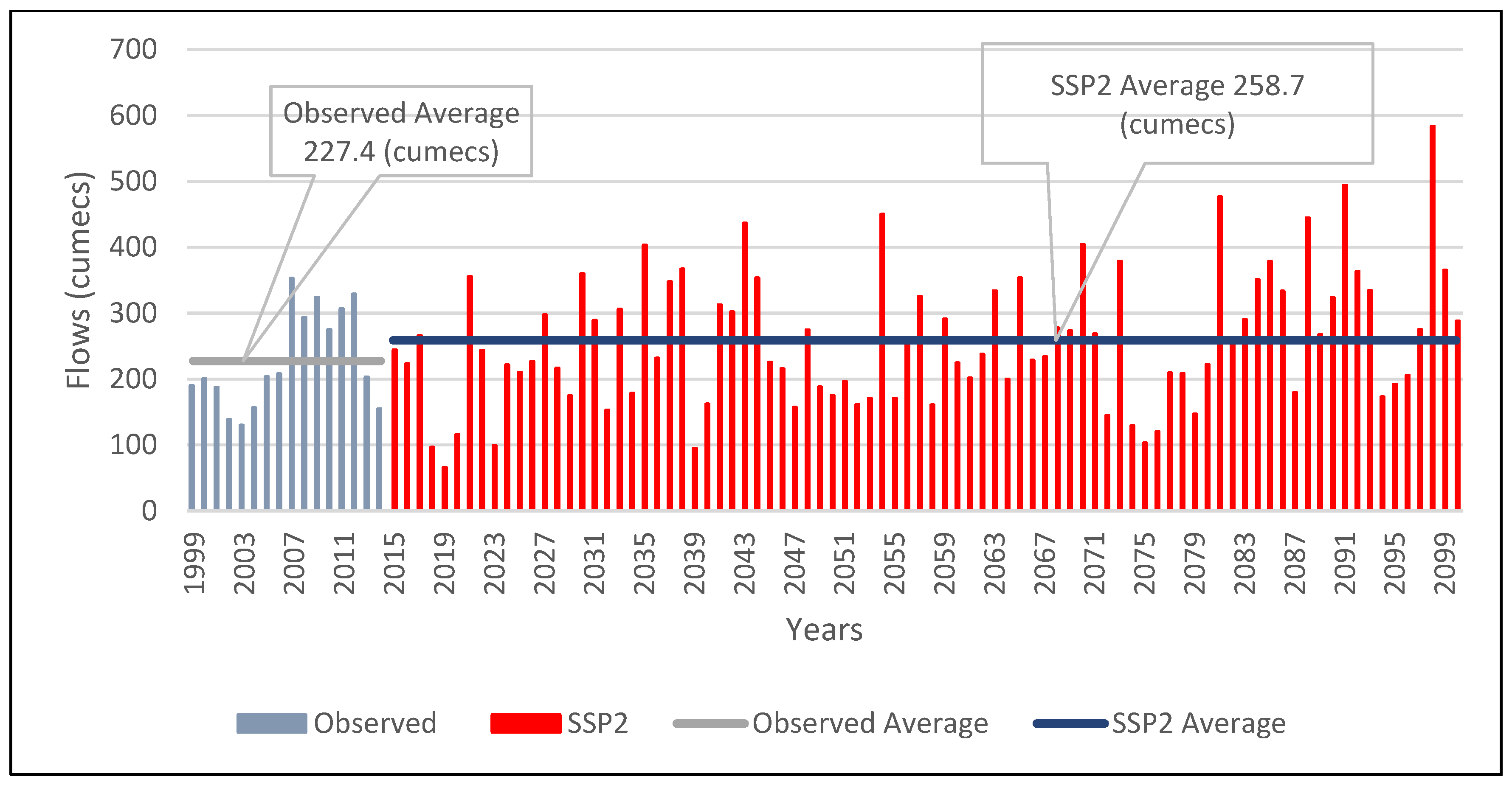
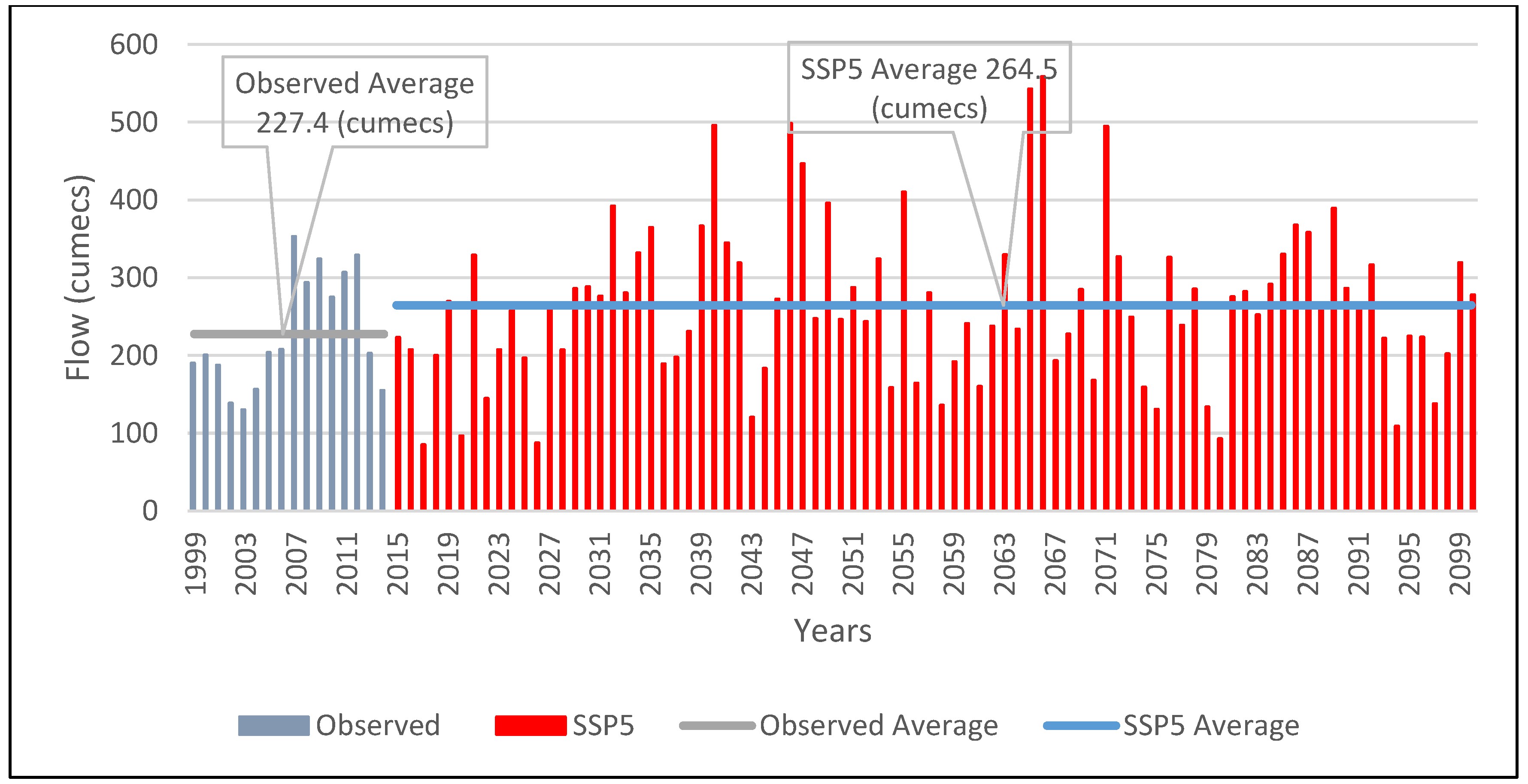
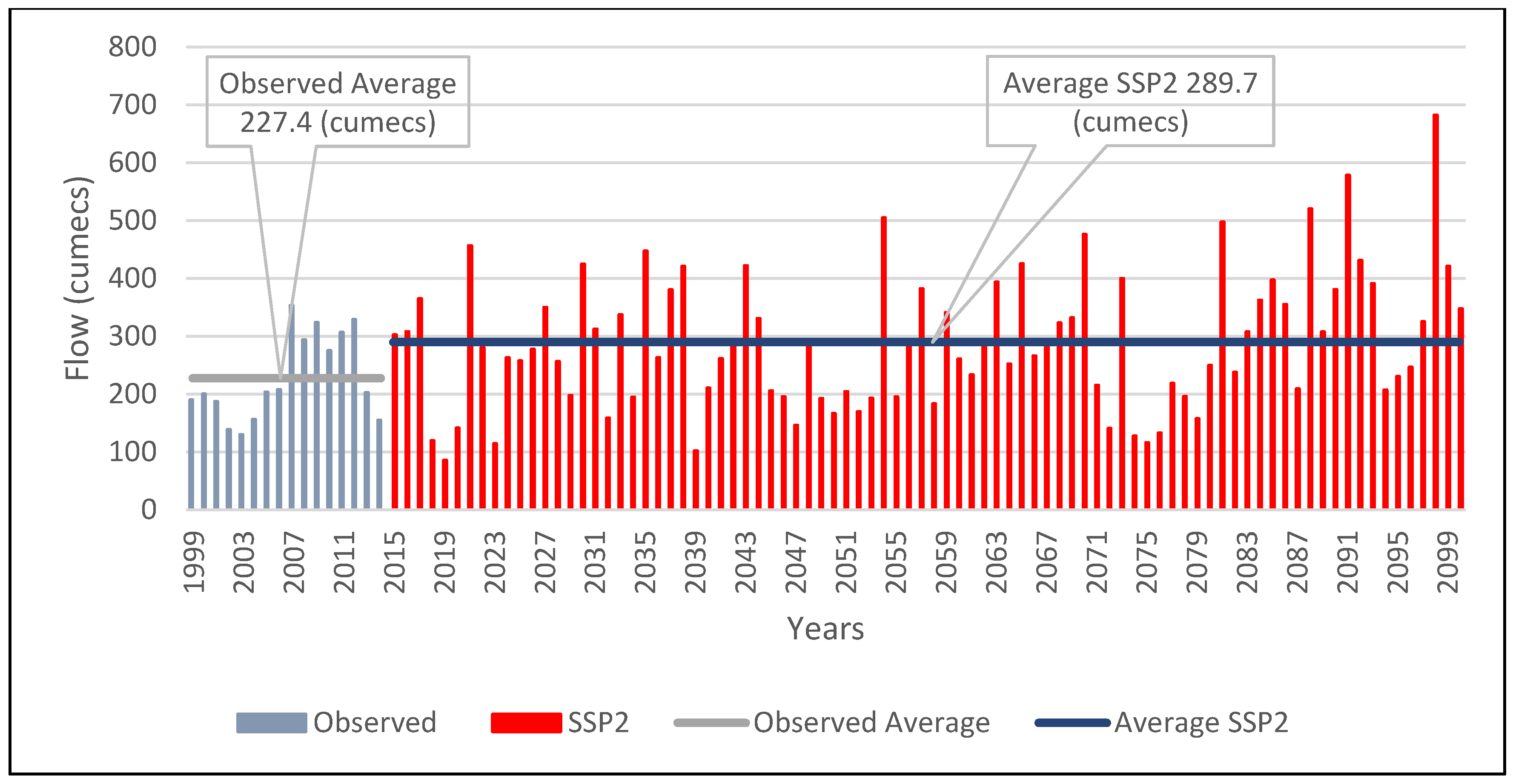
- The average daily streamflow at the Mohmand Dam site increased from 227.4 cumecs (1999–2015) to 258.7 cumecs under SSP2 and to 264.5 cumecs under SSP5 using the present land cover conditions;
- Under the future land cover change scenario, the flow increased from 227.4 cumecs (1999–2015) to 289.8 cumecs and 306.6 cumecs under SSP2 and SSP5, respectively;
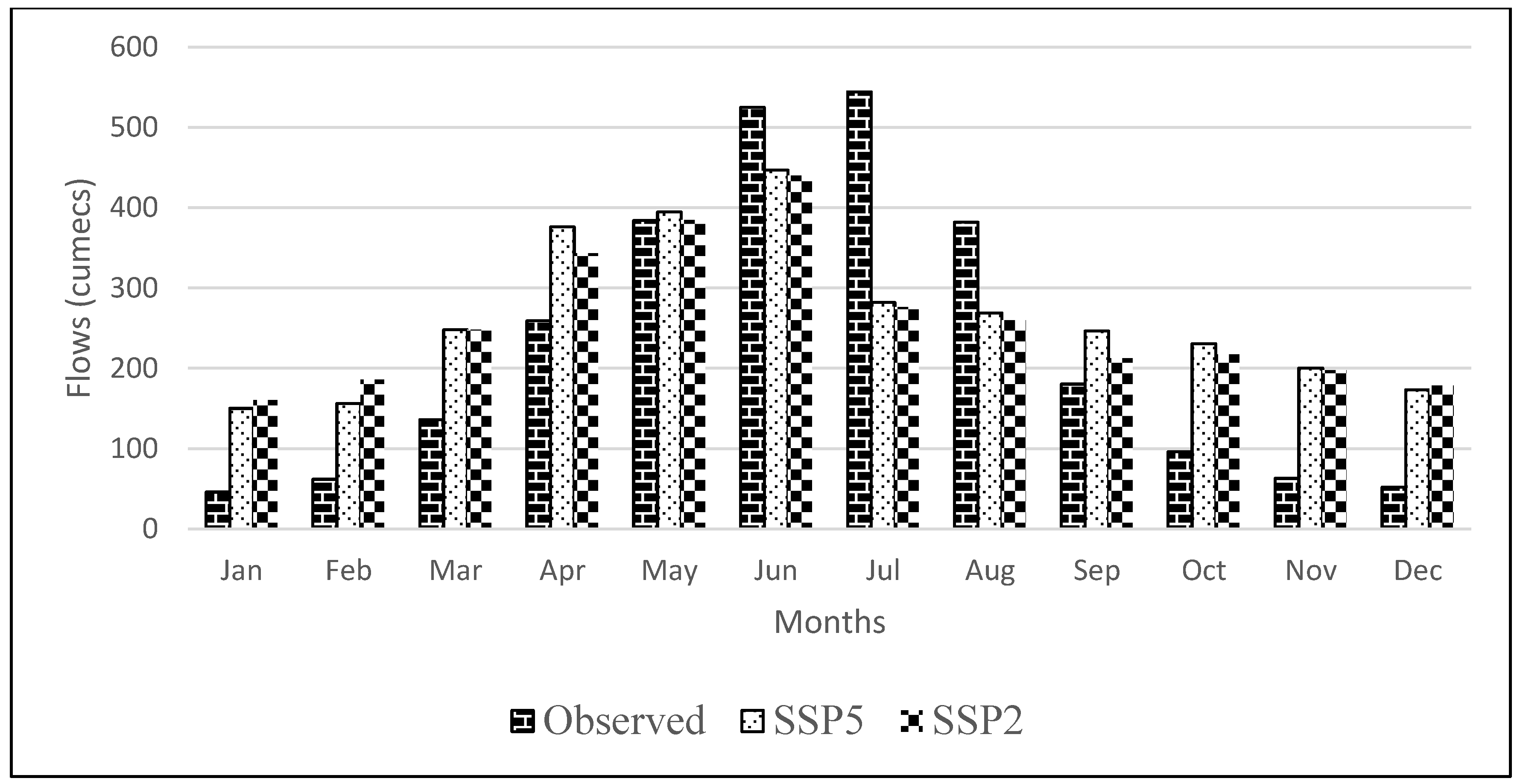
- The land cover and climate change scenarios results revealed that the overall mean monthly flows will increase by 27.4% and 34.8% under both SSPs, whereas the mean monthly flows in June, July and August will decrease (Figure 14), while the flows for November, December and January will increase under both SSPs (Figure 14); and
- The peak flow in the Mohmand Dam catchment is anticipated to advance by a month, i.e., from July to June in future scenarios of land cover and climate change conditions (Figure 14).
Author Contributions
Funding
Data Availability Statement
Conflicts of Interest
References
- Arheimer, B.; Donnelly, C.; Lindström, G. Regulation of snow-fed rivers affects flow regimes more than climate change. Nat. Commun. 2017, 8, 62. [Google Scholar] [CrossRef] [Green Version]
- Bolch, T. Asian glaciers are a reliable water source. Nature 2017, 545, 161–162. [Google Scholar] [CrossRef] [PubMed] [Green Version]
- Deng, H.; Chen, Y.; Wang, H.; Zhang, S. Climate change with elevation and its potential impact on water resources in the Tianshan Mountains, Central Asia. Glob. Planet. Chang. 2015, 135, 28–37. [Google Scholar] [CrossRef]
- Lutz, A.; Immerzeel, W.; Shrestha, A.B.; Bierkens, M.F. Consistent increase in High Asia’s runoff due to increasing glacier melt and precipitation. Nat. Clim. Chang. 2014, 4, 587–592. [Google Scholar] [CrossRef] [Green Version]
- Sharma, C.S.; Panda, S.N.; Pradhan, R.P.; Singh, A.; Kawamura, A. Precipitation and temperature changes in eastern India by multiple trend detection methods. Atmos. Res. 2016, 180, 211–225. [Google Scholar] [CrossRef]
- Haider, H.; Zaman, M.; Liu, S.; Saifullah, M.; Usman, M.; Chauhdary, J.; Anjum, M.; Waseem, M. Appraisal of Climate Change and its Impact on Water Resources of Pakistan: A Case Study of Mangla Watershed. Atmosphere 2020, 11, 1071. [Google Scholar] [CrossRef]
- Yao, T.D.; Thompson, L.; Yang, W.; Yu, W.S.; Gao, Y.; Guo, X.J.; Yang, X.X.; Duan, K.Q.; Zhao, H.B.; Xu, B.Q.; et al. Different glacier status with atmospheric circulations in Tibetan Plateau and surroundings. Nat. Clim. Chang. 2012, 2, 663–667. [Google Scholar] [CrossRef]
- Garee, K.; Chen, X.; Bao, A.; Wang, Y.; Meng, F. Hydrological Modeling of the Upper Indus Basin: A Case Study from a High-Altitude Glacierized Catchment Hunza. Water 2017, 9, 17. [Google Scholar] [CrossRef] [Green Version]
- Cheema, M.; Immerzeel, W.; Bastiaanssen, W. Spatial Quantification of Groundwater Abstraction in the Irrigated Indus Basin. Groundwater 2013, 52, 25–36. [Google Scholar] [CrossRef] [Green Version]
- Khan, A.; Naz, B.S.; Bowling, L.C. Separating snow, clean and debris covered ice in the Upper Indus Basin, Hindukush-Karakoram-Himalayas, using Landsat images between 1998 and 2002. J. Hydrol. 2015, 521, 46–64. [Google Scholar] [CrossRef] [Green Version]
- Ali, S.; Eum, H.-I.; Cho, J.; Dan, L.; Khan, F.; Dairaku, K.; Shrestha, M.L.; Hwang, S.; Nasim, W.; Khan, I.A.; et al. Assessment of climate extremes in future projections downscaled by multiple statistical downscaling methods over Pakistan. Atmos. Res. 2019, 222, 114–133. [Google Scholar] [CrossRef]
- Anjum, M.N.; Ding, Y.; Shangguan, D.; Ahmad, I.; Ijaz, M.W.; Farid, H.U.; Yagoub, Y.E.; Zaman, M.; Adnan, M. Performance evaluation of latest integrated multi-satellite retrievals for Global Precipitation Measurement (IMERG) over the northern highlands of Pakistan. Atmos. Res. 2018, 205, 134–146. [Google Scholar] [CrossRef]
- Tahir, A.A.; Adamowski, J.F.; Chevallier, P.; Haq, A.U.; Terzago, S. Comparative assessment of spatiotemporal snow cover changes and hydrological behavior of the Gilgit, Astore and Hunza River basins (Hindukush–Karakoram–Himalaya region, Pakistan). Meteorol. Atmos. Phys. 2016, 128, 793–811. [Google Scholar] [CrossRef]
- Dahri, Z.H.; Ludwig, F.; Moors, E.; Ahmad, B.; Khan, A.; Kabat, P. An appraisal of precipitation distribution in the high-altitude catchments of the Indus basin. Sci. Total. Environ. 2016, 548, 289–306. [Google Scholar] [CrossRef] [PubMed] [Green Version]
- Filippi, L.; Palazzi, E.; von Hardenberg, J.; Provenzale, A. Multidecadal Variations in the Relationship between the NAO and Winter Precipitation in the Hindu Kush–Karakoram. J. Clim. 2014, 27, 7890–7902. [Google Scholar] [CrossRef]
- Hasson, S.U.; Böhner, J.; Lucarini, V. Prevailing climatic trends and runoff response from Hindukush–Karakoram–Himalaya, upper Indus Basin. Earth Syst. Dyn. 2017, 8, 337–355. [Google Scholar] [CrossRef] [Green Version]
- Archer, D.R.; Forsythe, N.; Fowler, H.J.; Shah, S.M. Sustainability of water resources management in the Indus Basin under changing climatic and socio economic conditions. Hydrol. Earth Syst. Sci. 2010, 14, 1669–1680. [Google Scholar] [CrossRef] [Green Version]
- Ahmed, N.; Wang, G.; Booij, M.J.; Xiangyang, S.; Hussain, F.; Nabi, G. Separation of the Impact of Landuse/Landcover Change and Climate Change on Runoff in the Upstream Area of the Yangtze River, China. Water Resour. Manag. 2022, 36, 181–201. [Google Scholar] [CrossRef]
- Chernos, M.; MacDonald, R.J.; Straker, J.; Green, K.; Craig, J.R. Simulating the cumulative effects of potential open-pit mining and climate change on streamflow and water quality in a mountainous watershed. Sci. Total. Environ. 2022, 806, 150394. [Google Scholar] [CrossRef]
- Philip, E.; Rudra, R.P.; Goel, P.K.; Ahmed, S.I. Investigation of the Long-Term Trends in the Streamflow Due to Climate Change and Urbanization for a Great Lakes Watershed. Atmosphere 2022, 13, 225. [Google Scholar] [CrossRef]
- Ahmed, N.; Wang, G.; Lü, H.; Booij, M.J.; Marhaento, H.; Prodhan, F.A.; Ali, S.; Imran, M.A. Attribution of Changes in Streamflow to Climate Change and Land Cover Change in Yangtze River Source Region, China. Water 2022, 14, 259. [Google Scholar] [CrossRef]
- Shokouhifar, Y.; Lotfirad, M.; Esmaeili-Gisavandani, H.; Adib, A. Evaluation of climate change effects on flood frequency in arid and semi-arid basins. Water Supply 2022, 22, 6740–6755. [Google Scholar] [CrossRef]
- Baig, M.F.; Mustafa, M.R.U.; Baig, I.; Takaijudin, H.B.; Zeshan, M.T. Assessment of Land Use Land Cover Changes and Future Predictions Using CA-ANN Simulation for Selangor, Malaysia. Water 2022, 14, 402. [Google Scholar] [CrossRef]
- Azmat, M.; Liaqat, U.W.; Qamar, M.U.; Awan, U.K. Impacts of changing climate and snow cover on the flow regime of Jhelum River, Western Himalayas. Reg. Environ. Change 2016, 17, 813–825. [Google Scholar] [CrossRef]
- Ahmad, Z.; Hafeez, M.; Ahmad, I. Hydrology of mountainous areas in the upper Indus Basin, Northern Pakistan with the perspective of climate change. Environ. Monit. Assess. 2011, 184, 5255–5274. [Google Scholar] [CrossRef]
- Anjum, M.N.; Ding, Y.; Shangguan, D.; Liu, J.; Ahmad, I.; Ijaz, M.W.; Khan, M.I. Quantification of spatial temporal variability of snow cover and hydro-climatic variables based on multi-source remote sensing data in the Swat watershed, Hindukush Mountains, Pakistan. Meteorol. Atmos. Phys. 2018, 131, 467–486. [Google Scholar] [CrossRef]
- Rahman, M.A.; Yunsheng, L.; Sultana, N. Analysis and prediction of rainfall trends over Bangladesh using Mann–Kendall, Spearman’s rho tests and ARIMA model. Meteorol. Atmos. Phys. 2016, 129, 409–424. [Google Scholar] [CrossRef]
- Zhang, Y.; You, Q.; Chen, C.; Ge, J. Impacts of climate change on streamflows under RCP scenarios: A case study in Xin River Basin, China. Atmos. Res. 2016, 178, 521–534. [Google Scholar] [CrossRef]
- Almazroui, M.; Islam, M.N.; Saeed, F.; Alkhalaf, A.K.; Dambul, R. Assessing the robustness and uncertainties of projected changes in temperature and precipitation in AR5 Global Climate Models over the Arabian Peninsula. Atmos. Res. 2017, 194, 202–213. [Google Scholar] [CrossRef]
- Liu, Y.; Fan, K. An application of hybrid downscaling model to forecast summer precipitation at stations in China. Atmos. Res. 2014, 143, 17–30. [Google Scholar] [CrossRef]
- Xue, Y.; Janjic, Z.; Dudhia, J.; Vasic, R.; De Sales, F. A review on regional dynamical downscaling in intraseasonal to seasonal simulation/prediction and major factors that affect downscaling ability. Atmos. Res. 2014, 147, 68–85. [Google Scholar] [CrossRef] [Green Version]
- Akhtar, M.; Ahmad, N.; Booij, M. The impact of climate change on the water resources of Hindukush–Karakorum–Himalaya region under different glacier coverage scenarios. J. Hydrol. 2008, 355, 148–163. [Google Scholar] [CrossRef]
- Iqbal, M.; Wen, J.; Masood, M.; Masood, M.U.; Adnan, M. Impacts of Climate and Land-Use Changes on Hydrological Processes of the Source Region of Yellow River, China. Sustainability 2022, 14, 14908. [Google Scholar] [CrossRef]
- Haleem, K.; Khan, A.U.; Ahmad, S.; Khan, M.; Khan, F.A.; Khan, W.; Khan, J. Hydrological impacts of climate and land-use change on flow regime variations in upper Indus basin. J. Water Clim. Chang. 2021, 13, 758–770. [Google Scholar] [CrossRef]
- Mahmood, R.; Jia, S. Assessment of Impacts of Climate Change on the Water Resources of the Transboundary Jhelum River Basin of Pakistan and India. Water 2016, 8, 246. [Google Scholar] [CrossRef] [Green Version]
- Babur, M.; Babel, M.S.; Shrestha, S.; Kawasaki, A.; Tripathi, N.K. Assessment of Climate Change Impact on Reservoir Inflows Using Multi Climate-Models under RCPs—The Case of Mangla Dam in Pakistan. Water 2016, 8, 389. [Google Scholar] [CrossRef] [Green Version]
- Mahmood, R.; Jia, S.; Babel, M.S. Potential Impacts of Climate Change on Water Resources in the Kunhar River Basin, Pakistan. Water 2016, 8, 23. [Google Scholar] [CrossRef] [Green Version]
- Ahmad, I.; Zhang, F.; Tayyab, M.; Anjum, M.N.; Zaman, M.; Liu, J.; Farid, H.U.; Saddique, Q. Spatiotemporal analysis of precipitation variability in annual, seasonal and extreme values over upper Indus River basin. Atmos. Res. 2018, 213, 346–360. [Google Scholar] [CrossRef]
- Rozenberg, J.; Davis, S.J.; Narloch, U.; Hallegatte, S. Climate constraints on the carbon intensity of economic growth. Environ. Res. Lett. 2015, 10, 95006. [Google Scholar] [CrossRef] [Green Version]
- Basheer, A.K.; Lu, H.; Omer, A.; Ali, A.B.; Abdelgader, A.M.S. Impacts of climate change under CMIP5 RCP scenarios on the streamflow in the Dinder River and ecosystem habitats in Dinder National Park, Sudan. Hydrol. Earth Syst. Sci. 2016, 20, 1331–1353. [Google Scholar] [CrossRef] [Green Version]
- Diaz-Nieto, J.; Wilby, R.L. A comparison of statistical downscaling and climate change factor methods: Impacts on low flows in the River Thames, United Kingdom. Clim. Chang. 2005, 69, 245–268. [Google Scholar] [CrossRef]
- Anandhi, A.; Frei, A.; Pierson, D.C.; Schneiderman, E.M.; Zion, M.S.; Lounsbury, D.; Matonse, A.H. Examination of change factor methodologies for climate change impact assessment. Water Resour. Res. 2011, 47. [Google Scholar] [CrossRef] [Green Version]
- Zhang, Y.; Su, F.; Hao, Z.; Xu, C.; Yu, Z.; Wang, L.; Tong, K. Impact of projected climate change on the hydrology in the headwaters of the Yellow River basin. Hydrol. Process. 2015, 29, 4379–4397. [Google Scholar] [CrossRef]
- Moriasi, D.N.; Arnold, J.G.; Van Liew, M.W.; Bingner, R.L.; Harmel, R.D.; Veith, T.L. Model evaluation guidelines for systematic quantification of accuracy in watershed simulations. Trans. ASABE 2007, 50, 885–900. [Google Scholar] [CrossRef]
- Kumar, K.S.; Kumari, K.P.; Bhaskar, P.U. Application of Markov chain & cellular automata based model for prediction of Urban transitions. In Proceedings of the 2016 International Conference on Electrical, Electronics, and Optimization Techniques (ICEEOT), Chennai, India, 3–5 March 2016; pp. 4007–4012. [Google Scholar] [CrossRef]
- Tan, M.L.; Ibrahim, A.L.; Yusop, Z.; Chua, V.P.; Chan, N.W. Climate change impacts under CMIP5 RCP scenarios on water resources of the Kelantan River Basin, Malaysia. Atmos. Res. 2017, 189, 1–10. [Google Scholar] [CrossRef]
- Yang, T.; Hao, X.; Shao, Q.; Xu, C.-Y.; Zhao, C.; Chen, X.; Wang, W. Multi-model ensemble projections in temperature and precipitation extremes of the Tibetan Plateau in the 21st century. Glob. Planet. Change 2012, 80, 1–13. [Google Scholar] [CrossRef]
- Yan, L.; Liu, Z.; Chen, G.; Kutzbach, J.E.; Liu, X. Mechanisms of elevation-dependent warming over the Tibetan plateau in quadrupled CO2 experiments. Clim. Change 2016, 135, 509–519. [Google Scholar] [CrossRef]
- You, Q.; Min, J.; Kang, S. Rapid warming in the Tibetan Plateau from observations and CMIP5 models in recent decades. Int. J. Clim. 2015, 36, 2660–2670. [Google Scholar] [CrossRef] [Green Version]
- Dimri, A.; Kumar, D.; Choudhary, A.; Maharana, P. Future changes over the Himalayas: Maximum and minimum temperature. Glob. Planet. Chang. 2018, 162, 212–234. [Google Scholar] [CrossRef]
- Xin, J.; Gong, C.; Wang, S.; Wang, Y. Aerosol direct radiative forcing in desert and semi-desert regions of northwestern China. Atmos. Res. 2016, 171, 56–65. [Google Scholar] [CrossRef]
- Ozturk, T.; Turp, M.T.; Türkeş, M.; Kurnaz, M.L. Projected changes in temperature and precipitation climatology of Central Asia CORDEX Region 8 by using RegCM4.3.5. Atmos. Res. 2017, 183, 296–307. [Google Scholar] [CrossRef]
- Shamir, E.; Megdal, S.B.; Carrillo, C.; Castro, C.L.; Chang, H.-I.; Chief, K.; Corkhill, F.E.; Eden, S.; Georgakakos, K.P.; Nelson, K.M.; et al. Climate change and water resources management in the Upper Santa Cruz River, Arizona. J. Hydrol. 2015, 521, 18–33. [Google Scholar] [CrossRef] [Green Version]
- Kaskaoutis, D.; Houssos, E.; Solmon, F.; Legrand, M.; Rashki, A.; Dumka, U.; Francois, P.; Gautam, R.; Singh, R. Impact of atmospheric circulation types on southwest Asian dust and Indian summer monsoon rainfall. Atmos. Res. 2018, 201, 189–205. [Google Scholar] [CrossRef]
- Wang, C. Impact of anthropogenic absorbing aerosols on clouds and precipitation: A review of recent progresses. Atmos. Res. 2013, 122, 237–249. [Google Scholar] [CrossRef]
- Immerzeel, W.W.; Pellicciotti, F.; Bierkens, M.F.P. Rising river flows throughout the twenty-first century in two Himalayan glacierized watersheds. Nat. Geosci. 2013, 6, 742–745. [Google Scholar] [CrossRef]


| Sr. No. | Soil | Name | Texture | Area (km2) | Weightage of Area |
|---|---|---|---|---|---|
| 1 | I-B-U-2c-3503 | Lithosols | LOAM | 6517.53 | 46.7 |
| 2 | I-X-c-3512 | Lithosols | LOAM | 919.52 | 6.6 |
| 3 | Be70-2-3a-3667 | Haloic Cambisols | CLAY_LOAM | 1043.86 | 7.5 |
| 4 | Be73-2c-3673 | Eutric Cambisols | LOAM | 4464.06 | 32.0 |
| 5 | I-B-U-3712 | Calcaric Fluvisol | LOAM | 523.71 | 3.8 |
| 6 | Xh18-bc-3870 | Haplic Xerosols | SILT_LOAM | 220.86 | 1.6 |
| 7 | GLACIER-6998 | Gleysols | UWB | 266.75 | 1.9 |
| No. | Model Name | Institute | Nominal Resolution | Release Year |
|---|---|---|---|---|
| 1 | MIROC6 (Model for Interdisciplinary Research on Climate, 6th version) | National Institute for Environmental Studies and the Agency for Marine-Earth Science and Technology (MIROC), Japan | 250 km | 2017 |
| 2 | MPI-ESM1-2-HR (Max Planck Institute Earth System Model, version 1.2, high resolution) | Max Planck Institute for Meteorology, Germany | 100 km | 2017 |
| 3 | ACCESS-CM2 (Australian Community Climate and Earth System Simulator-Coupled Model, version 2) | Australian Community Climate and Earth System Simulator-Coupled Model, Australia | 250 km | 2016 |
| 4 | MRI-ESM2-0 (Meteorological Research Institute Earth System Model, version 2.0) | Meteorological Research Institute (MRI) of the Japan Meteorological Agency (JMA) | 100 km | 2017 |
| Model | R2 | NSE | PBIAS | MAE | RMSE |
|---|---|---|---|---|---|
| Access-CM2 | 0.09 | −0.81 | 0.73 | 71.38 | 113.56 |
| MIROC6 | 0.11 | −0.48 | −0.24 | 73.71 | 93.00 |
| MPI-ESM1-2-HR | 0.17 | 0.04 | 0.22 | 60.89 | 86.28 |
| MRI-ESM2 | 0.10 | −0.61 | −0.57 | 68.67 | 103.96 |
| Model | R2 | NSE | PBIAS | MAE | RMSE |
|---|---|---|---|---|---|
| Access-CM2 | 0.16 | −1.60 | 0.25 | 9.57 | 11.14 |
| MIROC6 | 0.20 | −1.64 | 0.39 | 10.05 | 19.61 |
| MPI-ESM1-2-HR | 0.26 | −0.58 | 0.06 | 7.62 | 9.00 |
| MRI-ESM2 | 0.19 | −1.58 | 0.20 | 8.55 | 11.05 |
| Model | R2 | NSE | PBIAS | MAE | RMSE |
|---|---|---|---|---|---|
| Access-CM2 | 0.14 | −0.93 | 0.46 | 12.36 | 12.40 |
| MIROC6 | 0.19 | −1.84 | 0.73 | 16.24 | 18.77 |
| MPI-ESM1-2-HR | 0.23 | −0.55 | 0.26 | 7.28 | 9.40 |
| MRI-ESM2 | 0.18 | −0.71 | 0.31 | 9.73 | 11.55 |
| Bias Correction for Precipitation | Bias Correction for Temperature |
|---|---|
|
|
| Model | Method | R2 | NSE | PBIAS | MAE | RMSE |
|---|---|---|---|---|---|---|
| MPI-ESM1 | Raw (model simulated historical) | 0.33 | 0.04 | 0.22 | 60.89 | 86.28 |
| Delta change | 0.68 | 0.60 | 0.10 | 31.72 | 46.83 | |
| Distribution mapping | 0.71 | 0.73 | 0.09 | 28.80 | 40.02 | |
| Linear scaling | 0.65 | 0.57 | 0.12 | 42.61 | 60.19 | |
| Power transformation | 0.75 | 0.74 | 0.04 | 19.42 | 29.44 | |
| Local intensity scaling | 0.66 | 0.58 | 0.11 | 36.27 | 53.47 |
| Model | Method | R2 | NSE | PBIAS | MAE | RMSE |
|---|---|---|---|---|---|---|
| MPI-ESM1 | Maximum temperature | |||||
| Raw (model simulated historical) | 0.38 | −0.58 | 0.06 | 7.62 | 9.00 | |
| Delta change | 0.68 | 0.36 | 0.20 | 3.69 | 5.72 | |
| Distribution mapping | 0.86 | 0.72 | 0.02 | 2.56 | 3.76 | |
| Linear scaling | 0.78 | 0.56 | 0.10 | 2.96 | 4.73 | |
| Variance scaling | 0.75 | 0.48 | 0.16 | 3.32 | 5.15 | |
| Minimum temperature | ||||||
| Raw (model simulated historical) | 0.33 | −0.55 | 0.26 | 7.28 | 9.40 | |
| Delta change | 0.64 | 0.29 | 0.18 | 3.58 | 6.40 | |
| Distribution mapping | 0.88 | 0.76 | 0.05 | 2.11 | 3.70 | |
| Linear scaling | 0.77 | 0.53 | 0.14 | 3.15 | 5.20 | |
| Variance scaling | 0.80 | 0.64 | 0.10 | 2.85 | 4.56 | |
| Parameters | Statistics | Historical | SSP2 | SSP5 |
|---|---|---|---|---|
| Precipitation | mm | 1136.05 | 1255.67 | 1269.51 |
| % Change | - | 10.5% | 11.7% | |
| Max Temperature | °C | 22.42 | 23.98 | 24.91 |
| % Change | - | 6.9% | 11.1% | |
| Min Temperature | °C | 7.92 | 9.20 | 10.01 |
| % Change | - | 16.1% | 26.3% |
| Parameter Name | Fitted Value | Min Value | Max Value |
|---|---|---|---|
| A__REVAPMN.gw | 200.225494 | 196 | 205 |
| V__ESCO.hru | 0.62635 | 0.4 | 0.7 |
| A__HRU_SLP.hru | 0.00882 | 0 | 0.12 |
| A__SLSUBBSN.hru | 58.1325 | 55 | 90 |
| V__CH_K2.rte | 138.827499 | 130 | 145 |
| V__SMFMN.bsn | 0.08125 | 0 | 6.5 |
| A__SURLAG.bsn | 12.341 | 11 | 17 |
| V__CN2.mgt | 89.525002 | 70 | 92 |
| V__CH_N2.rte | 0.09975 | 0 | 0.1 |
| V__SFTMP.bsn | 4.971110 | 4 | 5 |
| R__OV_N.hru | 0.09255 | 0 | 0.1 |
| R__SOL_BD(..).sol | 1.2704 | 0.9 | 2.5 |
| R__SOL_K(..).sol | 0.172985 | 0.16 | 0.23 |
| V__TLAPS.sub | −0.7918 | −1 | 0.2 |
| V__TIMP.bsn | 0.02755 | 0 | 0.1 |
| V__PLAPS.sub | 44.4375 | 25 | 50 |
| V__GW_DELAY.gw | 286.875 | 270 | 320 |
| V__SMFMX.bsn | 0.37575 | 0 | 4.5 |
| V__GWQMN.gw | 3990.625 | 3400 | 4150 |
| R__SOL_AWC(..).sol | 0.122825 | 0.11 | 0.3 |
| R__CANMX.hru | 47.57 | 30 | 50 |
| V__CH_N1.sub | 1.49275 | 1 | 3.7 |
| Calibration | Validation | |
|---|---|---|
| R2 | 0.81 | 0.78 |
| NSE | 0.79 | 0.74 |
| PBIAS | −10.6 | 11 |
Disclaimer/Publisher’s Note: The statements, opinions and data contained in all publications are solely those of the individual author(s) and contributor(s) and not of MDPI and/or the editor(s). MDPI and/or the editor(s) disclaim responsibility for any injury to people or property resulting from any ideas, methods, instructions or products referred to in the content. |
© 2023 by the authors. Licensee MDPI, Basel, Switzerland. This article is an open access article distributed under the terms and conditions of the Creative Commons Attribution (CC BY) license (https://creativecommons.org/licenses/by/4.0/).
Share and Cite
Masood, M.U.; Khan, N.M.; Haider, S.; Anjum, M.N.; Chen, X.; Gulakhmadov, A.; Iqbal, M.; Ali, Z.; Liu, T. Appraisal of Land Cover and Climate Change Impacts on Water Resources: A Case Study of Mohmand Dam Catchment, Pakistan. Water 2023, 15, 1313. https://doi.org/10.3390/w15071313
Masood MU, Khan NM, Haider S, Anjum MN, Chen X, Gulakhmadov A, Iqbal M, Ali Z, Liu T. Appraisal of Land Cover and Climate Change Impacts on Water Resources: A Case Study of Mohmand Dam Catchment, Pakistan. Water. 2023; 15(7):1313. https://doi.org/10.3390/w15071313
Chicago/Turabian StyleMasood, Muhammad Umer, Noor Muhammad Khan, Saif Haider, Muhammad Naveed Anjum, Xi Chen, Aminjon Gulakhmadov, Mudassar Iqbal, Zeshan Ali, and Tie Liu. 2023. "Appraisal of Land Cover and Climate Change Impacts on Water Resources: A Case Study of Mohmand Dam Catchment, Pakistan" Water 15, no. 7: 1313. https://doi.org/10.3390/w15071313