
Assessment of Regression Models for Surface Water Quality Modeling via Remote Sensing of a Water Body in the Mexican Highlands
 , , , ,
Abstract
:1. Introduction

| WQP | Surface (km2) | Resolution (m) | Sample of Size | Bands of Normalization | R2 | Estimation Interval (mg/L) | Author |
|---|---|---|---|---|---|---|---|
| TSS | 12,000 | 30 m | 26 | 0.98 | 0–386 | [45] | |
| 30 m | 14 | 0.69 | 0–135 | [22] | |||
| TN | 53 | 30 m | 18 | -------- | 0–36 | [3] | |
| TP | 53 | 30 m | 18 | -------- | 0–26 | [3] | |
| COD | 150 | 30 m | ------- | -------- | 0–19.3 | [19] |
2. Materials and Methods
2.1. Statistical Analysis for Model Development
2.2. Spatio-Temporal Distribution of Estimated WQPs
3. Results and Discussion
4. Conclusions
Author Contributions
Funding
Data Availability Statement
Acknowledgments
Conflicts of Interest
References
- Adjovu, G.E.; Stephen, H.; James, D.; Ahmad, S. Measurement of Total Dissolved Solids and Total Suspended Solids in Water Systems: A Review of the Issues, Conventional, and Remote Sensing Techniques. Remote Sens. 2023, 15, 3534. [Google Scholar] [CrossRef]
- Zeinalzadeh, K.; Rezaei, E. Determining spatial and temporal changes in surface water quality using principal component analysis. J. Hydrol. Reg. Stud. 2017, 13, 1–10. [Google Scholar] [CrossRef]
- Zeiny, A.; Kafrawy, S. Assessment of water pollution induced by human activities in Burullus Lake using Landsat 8 operational land imager and GIS. Egypt. J. Remote Sens. Space Sci. 2016, 20, 549–556. [Google Scholar]
- Ouma, Y.; Noor, K.; Herbert, K. Modelling Reservoir Chlorophyll-a, TSS, and Turbidity Using Sentinel-2A MSI and Landsat-8 OLI Satellite Sensors with Empirical Multivariate Regression. J. Sens. 2020, 2020, 8858408. [Google Scholar] [CrossRef]
- Gholizadeh, M.H.; Melesse, A.M.; Deddi, L. A Comprehensive Review on Water Quality Parameters Estimation Using Remote Sensing Techniques. Sensor 2016, 16, 1298. [Google Scholar] [CrossRef]
- Wang, X.; Yang, W. Water quality monitoring and evaluation using remote sensing techniques in China: A systematic review. Ecosyst. Health Sustain. 2019, 5, 47–56. [Google Scholar] [CrossRef]
- Yang, H.; Kong, J.; Hu, H.; Du, Y.; Gao, M.; Chen, F. A review of remote sensing for water quality retrieval: Progress and challenges. Remote Sens. 2022, 14, 1770. [Google Scholar] [CrossRef]
- Chang, N.B.; Imen, S.; Vannah, B. Remote Sensing for Monitoring Surface Water Quality Status and Ecosystem State in Relation to the Nutrient Cycle: A 40-Year Perspective. Crit. Rev. Environ. Sci. Technol. 2015, 45, 101–166. [Google Scholar] [CrossRef]
- Chang, N.B.; Bai, K.; Imen, S.; Chen, C.F.Y.; Gao, W. Fusión y creación de redes de imágenes satelitales multisensor para el monitoreo ambiental en todo clima. IEEE Syst. J. 2018, 12, 1341–1357. [Google Scholar] [CrossRef]
- Fauzi, M.; Wicaksono, P. Total Suspended Solid (TSS) Mapping of Wadaslintang Reservoir Using Landsat 8 OLI. In IOP Conference Series: Earth and Environmental Science-Proceedings of the 2nd International Conference of Indonesian Society for Remote Sensing (ICOIRS), Yogyakarta, Indonesia, 17–19 October 2016; IOP Publishing: Bristol, UK, 2019; Volume 47, pp. 1–9. [Google Scholar]
- Wang, H.; Wang, J.; Cui, Y.; Yan, S. Consistency of Suspended Particulate Matter Concentration in Turbid Water Retrieved from Sentinel-2 MSI and Landsat-8 OLI Sensors. Sensor 2021, 21, 1662. [Google Scholar] [CrossRef]
- Gómez, J.L.; Dalence, J.S. Determinación del parámetro sólidos suspendidos totales (SST) mediante imágenes de sensores ópticos en un tramo de la cuenca media del río Bogotá (Colombia). Rev. UD Geomática 2014, 9, 19–27. [Google Scholar]
- Torres Vera, M.A. Mapping of total suspended solids using Landsat imagery and machine learning. Int. J. Environ. Sci. Technol. 2023, 20, 11877–11890. [Google Scholar] [CrossRef]
- Xu, H.; Xu, G.; Hu, X.; Wang, Y. Lockdown effects on total suspended solids concentrations in the Lower Min River (China) during COVID-19 using time-series remote. Int. J. Appl. Earth Obs. Geoinf. 2021, 98, 102301. [Google Scholar] [CrossRef] [PubMed]
- Kumar, A.; Equeenuddin, S.M.; Mishra, D.R.; Acharya, B.C. Remote monitoring of sediment dynamics in a coastal lagoon: Long-term Spatio-temporal variability of suspended sediment in Chilika. Estuar. Coast. Shelf Sci. 2016, 170, 155–172. [Google Scholar] [CrossRef]
- Li, W.; Yu, W. Modelling Reservoir Turbidity Using Landsat 8 Satellite Imagery by Gene Expression Programming. Water 2019, 11, 1479. [Google Scholar] [CrossRef]
- Langhorst, T.; Pavelsky, T.; Eidam, E.; Cooper, L.; Davis, L.; Spellman, K.; Clement, S.; Arp, C.; Bondurant, A.; Friedmann, E.; et al. Increased scale and accessibility of sediment transport research in rivers through practical, open-source turbidity and depth sensors. Res. Square 2023, 1, 1–23. [Google Scholar] [CrossRef]
- Hajigholizadeh, M.; Melesse, A.M. Assortment and spatiotemporal analysis of surface water quality using. CATENA 2016, 151, 247–258. [Google Scholar] [CrossRef]
- Li, J.; Meng, Y.; Li, Y.; Cui, Q.; Yand, X.; Tao, C.; Wang, Z.; Li, l.; Zhang, W. Accurate water extraction using remote sensing imagery based on Normalized difference water index and unsupervised deep learning. J. Hydrol. 2022, 612, 128202. [Google Scholar] [CrossRef]
- Zhang, Y.; Wu, L.; Ren, H.; Deng, L.; Zhan, P. Retrieval of Water Quality Parameters from Hyperspectral Images Using Hybrid Bayesian Probabilistic Neural Network. Remote Sens. 2020, 12, 1567. [Google Scholar] [CrossRef]
- Chang, N.B.; Benjamin, W.; Jeffrey-Yang, Y.; Elovitz, M. Evaluation of dynamic linkages between evapotranspiration and land-use/land-cover changes with Landsat TM and ETM+ data. Int. J. Remote Sens. 2014, 33, 3733–3750. [Google Scholar]
- Jaelani, L.M.; Ratnaningsih, R.Y. Spatial and Temporal Analysis of Water Quality Parameter using Sentinel-2A Data; Case Study: Lake Matano and Towuti. Int. J. Adv. Sci. Eng. Inf. Technol. 2018, 8, 547–553. [Google Scholar] [CrossRef]
- Zheng, Z.; Wang, D.; Gong, F.; He, X.; Bai, Y. A Study on the Flux of Total Suspended Matter in the Padma River in Bangladesh Based on Remote-Sensing Data. Water 2021, 13, 2373. [Google Scholar] [CrossRef]
- Abdelmalik, K.W. Role of statistical remote sensing for Inland water quality parameters prediction. Egypt. J. Remote Sens. Space Sci. 2016, 21, 193–200. [Google Scholar] [CrossRef]
- Rahman, A.S.; Rahman, A. Application of Principal Component Analysis and Cluster Analysis in Regional Flood Frequency Analysis: A Case Study in New South Wales, Australia. Water 2020, 12, 781. [Google Scholar] [CrossRef]
- Sagan, V.; Peterson, K.T.; Maimaitijiang, M.; Sidike, P.; Sloan, J.; Greeling, B.A.; Adams, C. Monitoring inland water quality using remote sensing: Potential and limitations of spectral indices, bio-optical simulations, machine learning, and cloud computing. Earth-Sci. Rev. 2020, 205, 103187. [Google Scholar] [CrossRef]
- Bernardo, N.; Watanabe, F.; Rodrigues, T.; Alcántara, E. Atmospheric correction issues for retrieving total suspended matter concentrations in inland waters using OLI/Landsat-8 image. Adv. Space Res. 2017, 59, 2335–2348. [Google Scholar] [CrossRef]
- Chen, J.; Quan, W.; Duan, H.; Xing, Q.; Xu, N. An Improved Inherent Optical Properties Data Processing System for Residual Error Correction in Turbid Natural Waters. IEEE J. Sel. Top. Appl. Earth Obs. Remote Sens. 2021, 14, 6596–6607. [Google Scholar] [CrossRef]
- Wang, C.; Chen, S.; Li, D.; Wang, D.; Liu, W.; Yang, J. A Landsat-based model for retrieving total suspended concentration of estuaries and coasts in China. Geoscientific Model Dev. 2017, 10, 4347–4365. [Google Scholar] [CrossRef]
- Loaiza, J.G.; Rangel-Peraza, J.G.; Monjardín-Armenta, S.A.; Bustos-Terrones, Y.A.; Bandala, E.R.; Sanhouse-García, A.J.; Rentería-Guevara, S.A. Surface Water Quality Assessment through Remote Sensing Based on the Box–Cox Transformation and Linear Regression. Water 2023, 15, 2606. [Google Scholar] [CrossRef]
- Chongyang, W.; Weijiao, L.; Shuisen, C.; Dan, L.; Danni, W.; Jia, L. The spatial and temporal variation of total suspended solid concentration in Pearl River Estuary during 1987–2015 based on remote sensing. Sci. Total Environ. 2018, 618, 1125–1138. [Google Scholar]
- Ghada, Y.E.; Marieke, A.E.; Meinte, B.; Kessel, T.; Gaytan, S.; Hendrik, J. Improving the Description of the Suspended Particulate Matter Concentrations in the Southern North Sea through Assimilating Remotely Sensed Data. Ocean Sci. J. 2011, 46, 179–204. [Google Scholar]
- Cahyono, B.; Jamilah, U.L.; Nugroho, M.A.; Subekti, A. Analysis of Total Suspended Solids (TSS) at Bedadung River, Jember District of Indonesia Using Remote Sensing Sentinel 2A Data. Singap. J. Sci. Res. 2019, 9, 117–123. [Google Scholar]
- Saberioon, M.; Brom, J.; Nedbal, V.; Soucek, P.; Cízar, P. Chlorophyll-a and total suspended solids retrieval and mapping using Sentinel-2A and machine learning for inland waters. Ecol. Indic. 2020, 113, 106236. [Google Scholar] [CrossRef]
- Vakili, T.; Amanollahi, J. Determination of optically inactive water quality variables using Landsat 8 data: A case study in Geshlagh reservoir affected by agricultural land use. J. Clean. Prod. 2019, 247, 119134. [Google Scholar] [CrossRef]
- Zhao, J.; Zhang, F.; Chen, S.; Wang, C.; Chen, J.; Zhou, H.; Xue, Y. Remote Sensing Evaluation of Total Suspended Solids Dynamic with Markov Model: A Case Study of Inland Reservoir across Administrative Boundary in South China. Sensors 2020, 20, 6911. [Google Scholar] [CrossRef]
- Pizani, F.C.; Ferreira, A.F.; Amorim, C.C. Estimation of water quality in a reservoir from Sentinel-2 MSI and Landsat 8-OLI Sensor. SPRS Ann. Photogramm. Remote Sens. Spat. Inf. Sci. 2020, 3, 401–408. [Google Scholar] [CrossRef]
- Ekercin, S. Water Quality Retrievals from High-Resolution Ikonos Multispectral Imagery: A Case Study in Istanbul, Turkey. Water Air Soil Pollut. 2007, 183, 239–251. [Google Scholar] [CrossRef]
- Carrillo, I.D.; Medina, R.J. Multitemporal analysis of the flow of sediments using modis MYD09 and MOD09 images. Cienc. Ing. Neogranadina-Univ. Mil. Nueva Guin. 2019, 29, 69–86. [Google Scholar] [CrossRef]
- Yeboah, Y.; Quaye-Ballard, J.; Amatey, A.; Appiah, A. Spatial prediction mapping of water quality of Owabi reservoir from satellite imageries and machine learning models. Egypt. J. Remote Sens. Space Sci. 2021, 24, 825–833. [Google Scholar]
- Nguyen, T.H.; Phan, D.; Nguyen, H.T.; Tran, S.; Tran, T.; Tran, B.; Doan, T. Total Suspended Solid Distribution in au River Using Sentinel 2A Satellite Imagery. ISPRS Ann. Photogramm. Remote Sens. Spat. Inf. Sci. 2020, 4, 91–97. [Google Scholar] [CrossRef]
- Markogianni, V.; Kalivas, D.; Petropoulos, G.; Dimitriou, E. Analysis on the Feasibility of Landsat 8 Imagery for Water Quality Parameters Assesment in an Oligotrophic Mediterranean Lake. Int. J. Geol. Environ. Eng. 2017, 11, 906–914. [Google Scholar]
- Wang, D.; Ma, R.; Xue, K.; Loiselle, S.A. The Assessment of Landsat-8 OLI Atmospheric Correction Algorithms for Inland Waters. Remote Sens. 2019, 11, 169. [Google Scholar] [CrossRef]
- Kavurmacı, M.; Karakuş, C.B. Evaluación de la calidad del agua de riego mediante análisis envolvente de datos e índices de calidad del agua basados en procesos de jerarquía analítica: El caso de la ciudad de Aksaray, Turquía. Contam. Agua Aire Suelo 2020, 55, 1–123. [Google Scholar]
- Ruiz, D.C. Method of Estimating Total Suspended Solids as an Indicator of Water Quality Using Satellite Images. In Reposiorio Institucional-Biblotteca Digital; National University of Colombia: Bogotá, Colombia, 2017; pp. 1–47. [Google Scholar]
- Fernández, A.; Moreira, J.M. Methodology for the Multitemporal Monitoring of the Quality of Coastal Waters in Andalusia through Landsat-TM Image Processing; Remote Sensing Uses and Applications, University of Seville; Deposito de Investigation Universidad de Sevilla: Seville, Spain, 2014; Volume 1, pp. 1–65. [Google Scholar]
- Lu, H.; Liu, Q.; Liu, X.Y.; Zhang, Y. Un estudio sobre la construcción semántica y la aplicación de imágenes y datos de teledetección por satélite. Rev. De Informática Organ. Usuario Final. (JOEUC) 2021, 33, 1–20. [Google Scholar]
- Hernandez, J. Methodology for the Evaluation of Volumetric and Energy Impacts Inflows by Transfer: Case Study Upper Course of the Lerma River. Master’s Thesis, Inter-American Water Resources Center/UAEMex, Toluca, Mexico, 2018. (In Spanish). [Google Scholar]
- Ciancia, E.; Campanelli, A.; Lacava, T.; Palombo, A.; Pascucci, S.; Pergola, N.; Tramutoli, V. Modeling and Multi-Temporal Characterization of Total Suspended Matter by the Combined Use of Sentinel 2-MSI and Landsat 8-OLI Data: The Pertusillo Lake Case Study (Italy). Remote Sens. 2020, 12, 2147. [Google Scholar] [CrossRef]
- Doña, C. Monitoring water quality and hydrological patterns of wetlands using recent techniques in remote sensing. In Departament de Física de la Terra i Termodinàmica; Universitat Valencia: Valencia, Spain, 2016; pp. 1–93. [Google Scholar]
- DOF. Water Analysis—Measurement of Total Nitrogen Kjeldahl in Natural Water, Wastewater and Treated Wastewater—Test Method; Ministry of Economy: Mexico City, Mexico, 2010. (In Spanish)
- DOF. Water Analysis—Measurement of Dissolved Solids and Salts in Natural Water, Wastewater, and Treated Wastewater—Test Method; Ministry of Economy: Mexico City, Mexico, 2015. (In Spanish)
- DOF. Water Analysis—Measurement of Total Phosphorus in Natural Water, Wastewater, and Treated Wastewater—Test Method; Ministry of Economy: Mexico City, Mexico, 2001. (In Spanish)
- DOF. Water Analysis—Measurement of Chemical Oxigen Demand in Natural Water, Wastewater, and Treated Wastewater—Test Method; Ministry of Economy: Mexico City, Mexico, 2012. (In Spanish)
- NOM-001-SEMARNART-2021; Official Mexican Standard. SEGOB: Mexico City, Mexico, 2023. (In Spanish)
- Kim, Y.; Im, J.; Ha, H.K.; Choi, J.-K.; Ha, S. Machine learning approaches to coastal water quality monitoring using GOCI Satellite data. GIS Sci. Remote Sens. 2014, 51, 158–174. [Google Scholar] [CrossRef]
- Li, C.; Rousta, I.; Olafsoon, H.; Zhang, H. Lake Water Quality and Dinamics Assesssment during 1990–2020 (A case Study: Chao Lake: China). Atmosphere 2023, 14, 382. [Google Scholar] [CrossRef]
- Li, L.; Gu, M.; Gong, C.; Hu, Y.; Wang, X.; Yang, Z.; He, Z. An advanced remote sensing retrieval method for urban non-optically active water quality parameters: An example from Shanghai. Sci. Total Environ. 2023, 880, 163389. [Google Scholar] [CrossRef]
- Mun, J. Risk Simulator User Manual in Spanish; R-Real Options Valuation: Dublin, Ireland, 2012. [Google Scholar]
- Swain, R.; Sahoo, B. Improving river water quality monitoring using satellite data product and a genetic algorithm processing aproach. Sustain. Water Qual. Ecol. 2017, 10, 122–149. [Google Scholar]
- IBM. IBM SPSS Statistics 28 Brief Guide; IBM Corporation: Endicott, NY, USA, 2021; Volume 1, pp. 1–90. [Google Scholar]
- Zou, D.; Lloyd, J.V.; Baumbusch, J.L. Using SPSS to analyze Complex Survey Data: A Primer. J. Mod. Appl. Stat. Methods 2019, 18, 16. [Google Scholar] [CrossRef]
- Aiman, M.; Mohosen, M.; Hossam, S. Statistical estimation of Rosetta Branch Water Quality using multi-spectral data. Water Sci. 2014, 28, 18–30. [Google Scholar]
- CONAGUA. (1 July 2019). National Water Commission. Available online: https://app.conagua.gob.mx/bandas/ (accessed on 14 April 2021).
- Tu, M.C.; Smith, P.; Filippi, A.M. Hybrid forward-selection method-based water-quality estimation via combining Landsat TM, ETM+, and OLI/TIRS images and ancillary environmental data. PLoS ONE 2018, 13, e0201255. [Google Scholar] [CrossRef] [PubMed]
- Sundarabalan, V.; Pahlevan, N.; Smith, B.; Binding, C.; Schalles, J.; Loisel, H.; Boss, E. Robust algorithm for estimating total suspended solids (TSS) in inland and nearshore coastal waters. Remote Sens. Environ. 2020, 246, 111768. [Google Scholar]


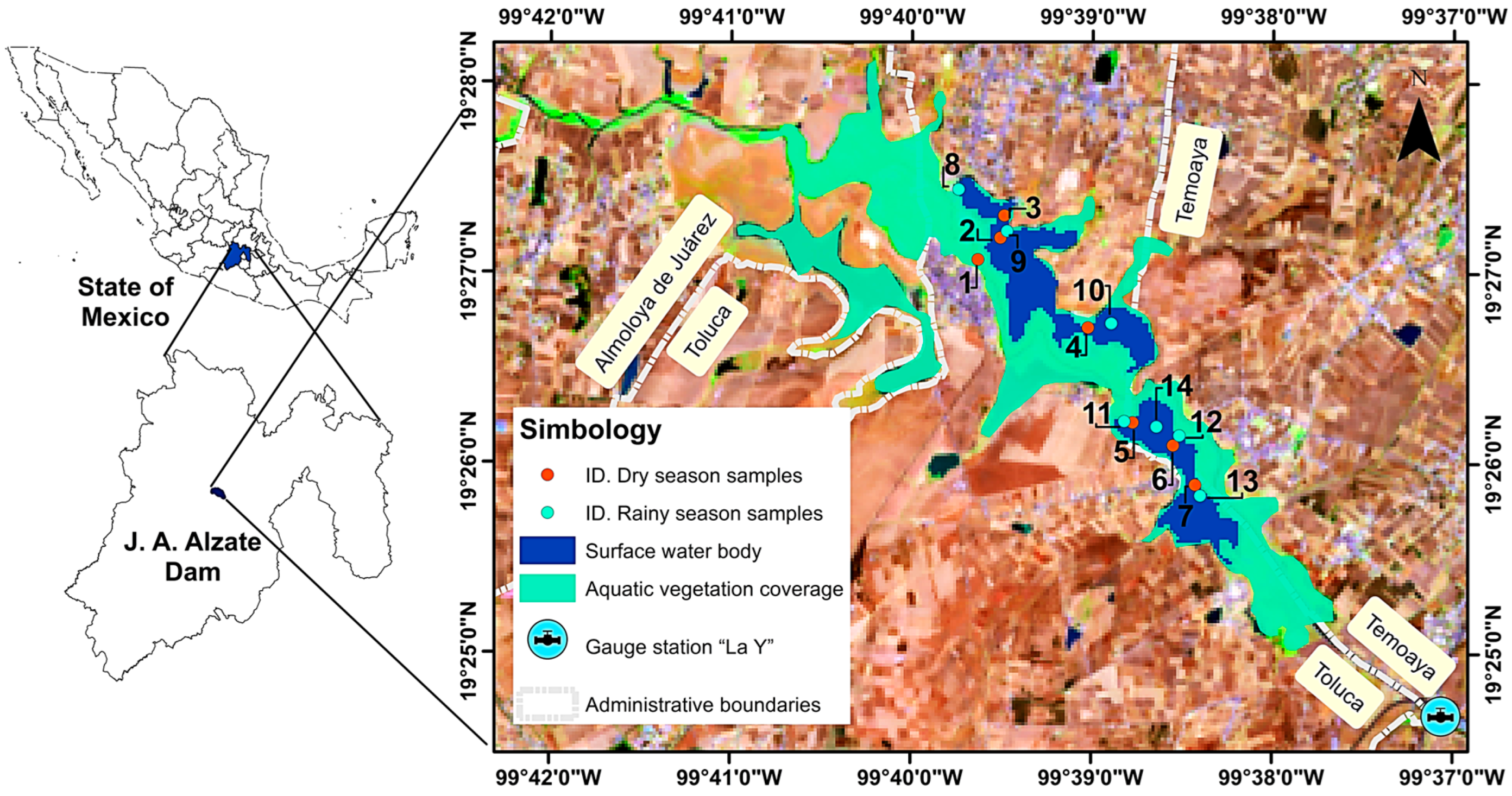
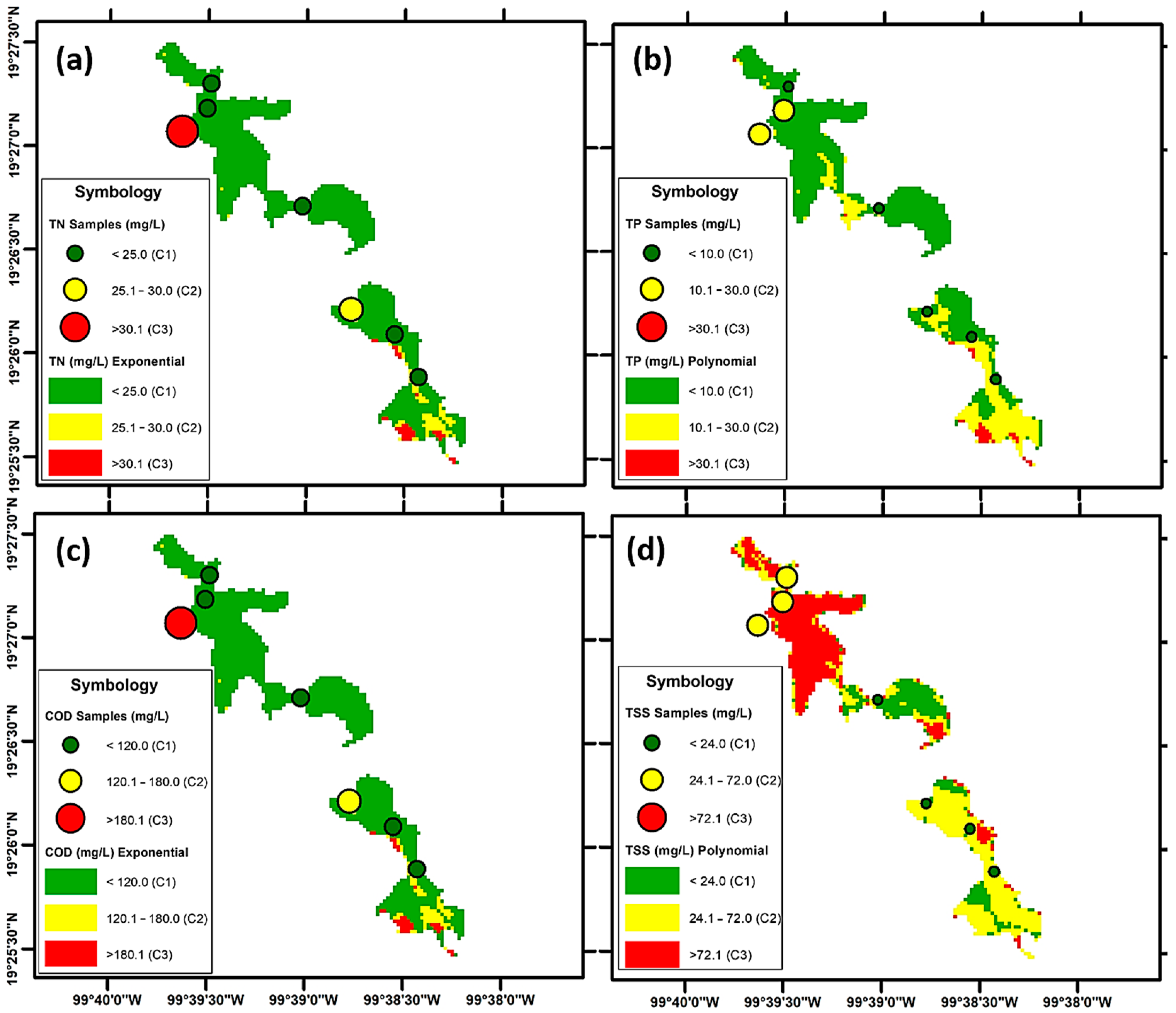
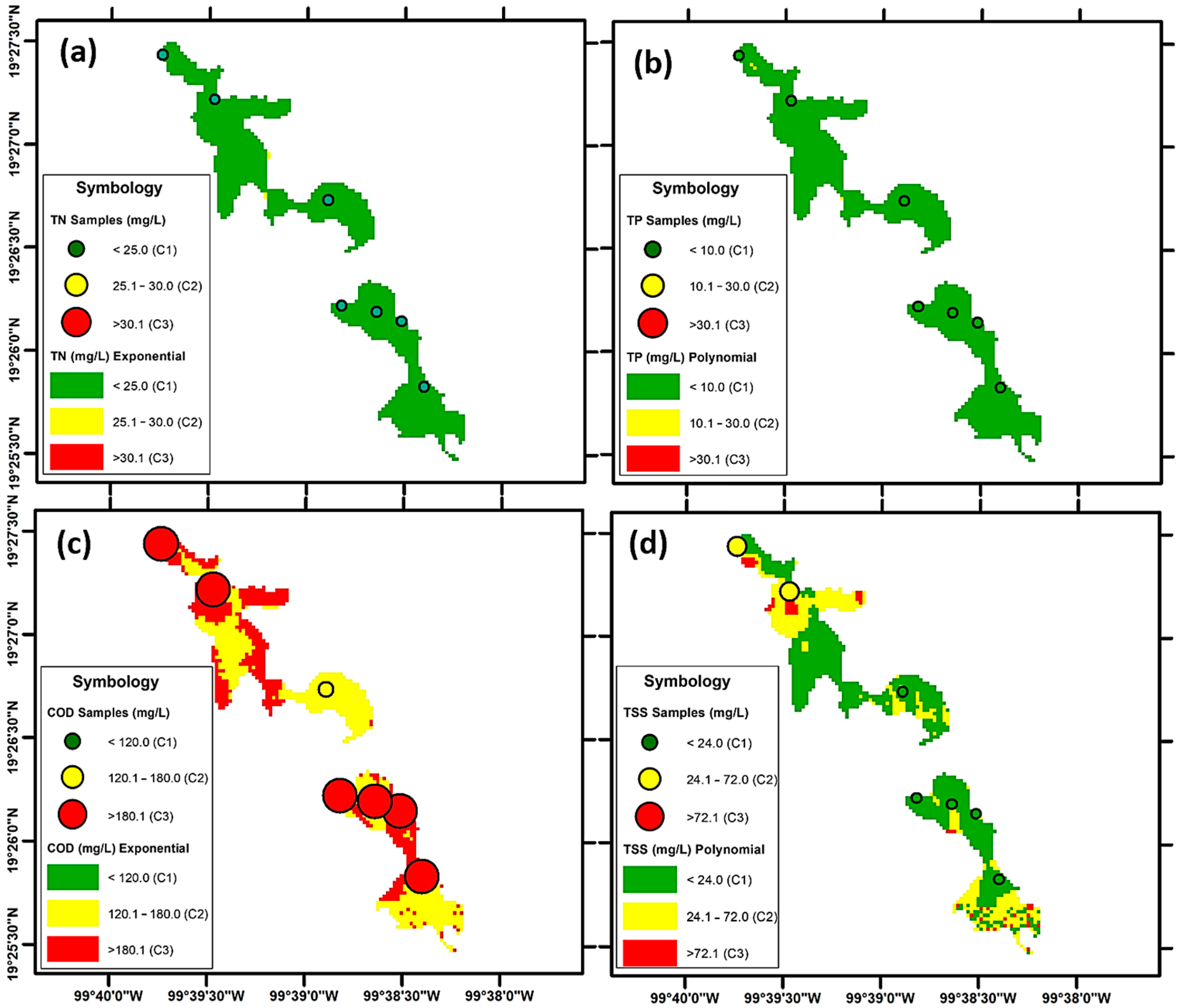
| ID | X (W Longitude) | Y (N Latitude) | Season | Chemistry Parameters | Physics p. | ||
|---|---|---|---|---|---|---|---|
| TN (mg/L) | COD (mg/L) | TP (mg/L) | TSS (mg/L) | ||||
| PL = 40–60 | PL = 60–75 | PL = 20–30 | PL = 12–75 | ||||
| 1 | −99.660564 | 19.451172 | Before the rain season 18th May | 33 | 173 | 99.76 | 92.5 |
| 2 | −99.658486 | 19.453087 | 11 | 127 | 46.27 | 151.5 | |
| 3 | −99.658131 | 19.455031 | 16 | 66 | 44.34 | 198 | |
| 4 | −99.650393 | 19.445229 | 9 | 93 | 34.25 | 48 | |
| 5 | −99.646237 | 19.436919 | 28 | 107 | 70.91 | 33 | |
| 6 | −99.642504 | 19.434917 | 20 | 98 | 67.34 | 55 | |
| 7 | −99.640462 | 19.431472 | 10 | 109 | 74.92 | 42 | |
| 8 | −99.662355 | 19.457317 | After the rain season 26th October | 7.2 | 67.5 | 33.16 | 35 |
| 9 | −99.657869 | 19.453669 | 6.3 | 64 | 34.46 | 34 | |
| 10 | −99.648234 | 19.445605 | 3.9 | 80 | 23.64 | 15.2 | |
| 11 | −99.644043 | 19.436555 | 4.4 | 21 | 30.76 | 11 | |
| 12 | −99.641932 | 19.435785 | 3.5 | 30 | 32.79 | 16 | |
| 13 | −99.639985 | 19.430514 | 2.8 | 26 | 30.39 | 17 | |
| 14 | −99.647021 | 19.437027 | 3.3 | 39.5 | 33.71 | 19 | |
| Statistical Test | WQP | Total Nitrogen (TN) | Chemistry Oxygen Demand (COD) | |||||||||||||||||
|---|---|---|---|---|---|---|---|---|---|---|---|---|---|---|---|---|---|---|---|---|
| Model Type | Exponential | Linear | Polynomial | Exponential | Linear | Polynomial | ||||||||||||||
| Independent Variables | B1, B3 | B3, B6, (B3 + B7) | (B1/B3) | LN(B5), LN(B2/B3), LN(B7) | (B1/B6), (B7/B4), (B2/B1), (B2/B3) | (B3/B1), (B3/B5) | ||||||||||||||
| Vcrit | V | Vcrit | V | Vcrit | V | Vcrit | V | Vcrit | V | Vcrit | V | |||||||||
| Homoscedasticity | W-pvalue > Vcrit | 0.1 | 0.25 | 0.1 | 0.33 | 0.1 | 0.23 | 0.1 | 0.18 | 0.1 | 0.25 | 0.1 | 0.38 | |||||||
| Square chi test | χ2 < Vcrit | 7.81 | 4.54 | 7.81 | 4.65 | 11.07 | 9.30 | 7.81 | 2.25 | 9.48 | 2.26 | 11.07 | 0.82 | |||||||
| Atypical values | Vcalc ≤ Vcrit | 2 | 1 | 2 | 1 | 2 | 1 | 2 | 1 | 2 | 0 | 2 | 1 | |||||||
| Collinearity | VIF < Vcrit | 4 | 0.21 | 4 | 0.16 | 4 | 4.0 | 4 | 0.21 | 4 | 2.6 | 4 | 1.17 | |||||||
| r ≤ Vcrit | 0.75 | 0.74 | 0.75 | 0.75 | 0.75 | 0.86 | 0.75 | 0.74 | 0.75 | 0.78 | 0.75 | 0.78 | ||||||||
| Multicollinearity | F > Vcrit | 3.70 | 22.90 | 3.70 | 13.20 | 3.68 | 6.25 | 3.70 | 19.08 | 3.63 | 6.75 | 3.68 | 11.82 | |||||||
| Normality | D < Vcrit | 0.22 | 0.12 | 0.22 | 0.17 | 0.17 | 0.22 | 0.22 | 0.19 | 0.22 | 0.08 | 0.22 | 0.16 | |||||||
| Significance | Pvalue ≤ Vcrit | 0.05 | 0.19 | 0.05 | 0.05 | 0.05 | 0.06 | 0.05 | 0.00 | 0.05 | 0.09 | 0.05 | 0.79 | |||||||
| Statistical Test | WQP | Total Phosphorus (TP) | Total Suspended Solids (TSS) | |||||||||||||||||
| Model Type | Exponential | Linear | Polynomial | Exponential | Linear | Polynomial | ||||||||||||||
| Independent Variables | LN(B5), LN(B6) | (B5/B4), (B5/B6) | (B5/B2), (B5/B2) | LN(B4), LN(B3+B5), LN(B5+B7), LN(B2/B3), LN(B2/B4) | (B7/B4), (B7/B5) | (B3/B5), B3 | ||||||||||||||
| Vcrit | V | Vcrit | V | Vcrit | V | Vcrit | V | Vcrit | V | Vcrit | V | |||||||||
| Homoscedasticity | W-pvalue > Vcrit | 0.1 | 0.18 | 0.1 | 0.64 | 0.1 | 0.10 | 0.1 | 0.11 | 0.1 | 0.11 | 0.1 | 0.12 | |||||||
| Square chi test | χ2 < Vcrit | 5.99 | 4.87 | 5.99 | 2.62 | 11.07 | 5.61 | 11.07 | 5.93 | 3.32 | 5.99 | 11.07 | 1.90 | |||||||
| Atypical values | Vcalc ≤ Vcrit | 2 | 1 | 2 | 0 | 2 | 1 | 2 | 1 | 2 | 0 | 2 | 1 | |||||||
| Collinearity | FIV < Vcrit | 4 | 2.63 | 4 | 6.31 | 4 | 2.88 | 4 | 4.1 | 4 | 1.28 | 4 | 1.38 | |||||||
| r ≤ Vcrit | 0.75 | 0.78 | 0.75 | 0.9 | 0.75 | 0.80 | 0.75 | 0.87 | 0.75 | 0.46 | 0.75 | 0.52 | ||||||||
| Multicollinearity | F > Vcrit | 3.98 | 18.65 | 3.98 | 24.3 | 3.68 | 25.63 | 3.68 | 30.60 | 3.98 | 11.28 | 3.68 | 136.12 | |||||||
| Normality | D < Vcrit | 0.22 | 0.16 | 0.23 | 0.22 | 0.22 | 0.12 | 0.22 | 0.15 | 0.22 | 0.20 | 0.22 | 0.15 | |||||||
| Significance | Pvalue ≤ Vcrit | 0.05 | 0.00 | 0.05 | 0.003 | 0.05 | 0.00 | 0.05 | 0.04 | 0.05 | 0.07 | 0.05 | 0.09 | |||||||
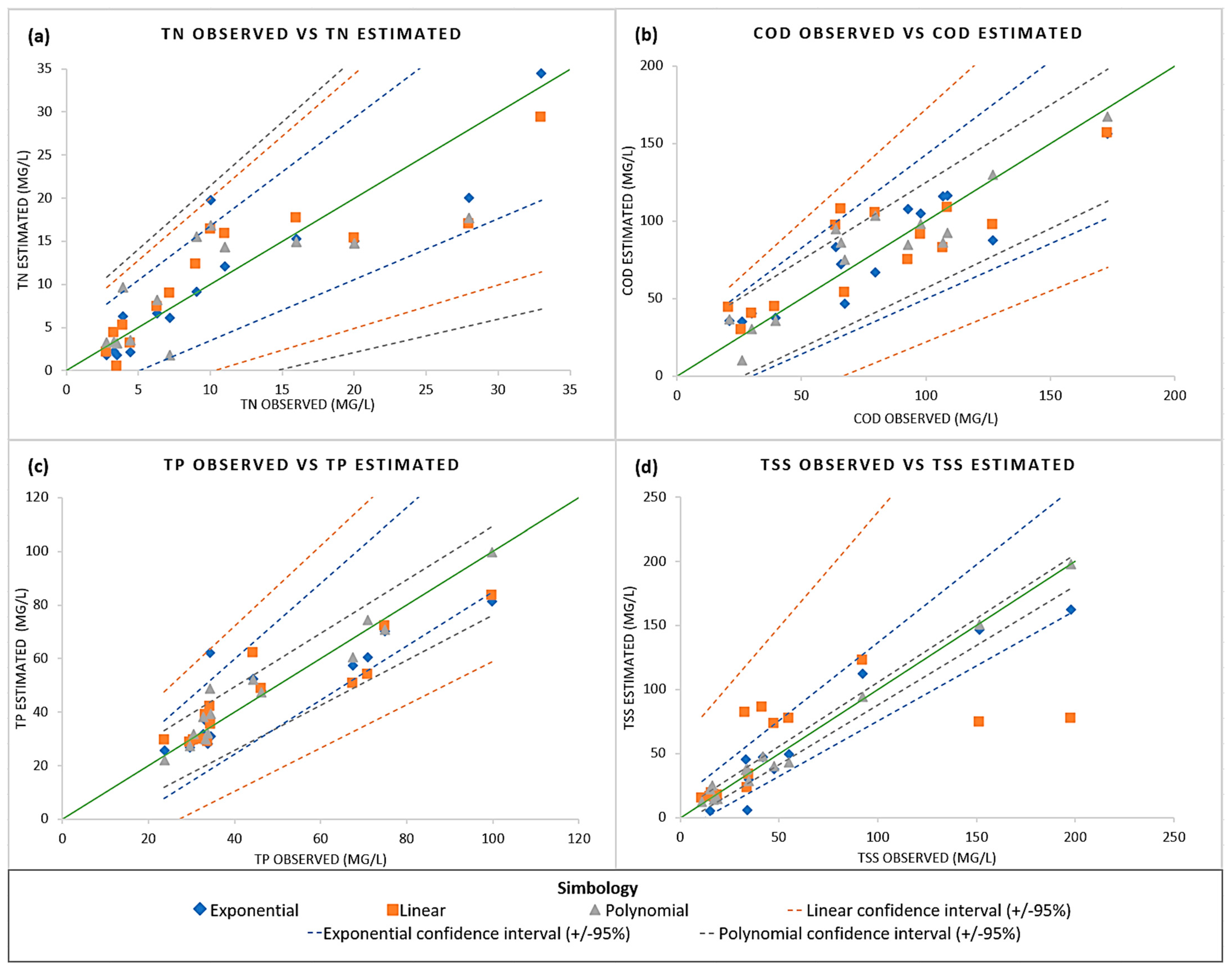
| WQP | Type | Regression Model | RMSE | ||
|---|---|---|---|---|---|
| TN (mg/L) | Exp. | 5 | 3.82 | 0.79 | |
| Linear | 7 | 4.24 | 0.73 | ||
| Pol. | 14 | 31.13 | 0.68 | ||
| COD (mg/L) | Exp. | 6 | 16.1 | 0.80 | |
| Linear | 5 | 21.4 | 0.62 | ||
| Pol. | 9 | 15.35 | 0.84 | ||
| TP (mg/L) | Exp. | 8 | 10.25 | 0.74 | |
| Linear | 5 | 9.63 | 0.79 | ||
| Pol. | 5 | 5.49 | 0.92 | ||
| TSS (mg/L) | Exp. | 5 | 14.37 | 0.90 | |
| Linear | 5 | 43.9 | 0.61 | ||
| Pol. | 6 | 7.19 | 0.98 |
| WQP | Mean in Samples (mg/L) | Standard Deviation (mg/L) | Confidence Interval for Difference in Means (mg/L) | Author | |||
|---|---|---|---|---|---|---|---|
| A.M. | C.M. | A.M. | C.M. | ||||
| TSS | 11.06 | 15.74 | 22.79 | 8.81 | −9.51 | 0.57 | [45] |
| TN | 23.71 | 26.99 | 1.36 | 0.94 | −3.62 | −2.94 | [3] |
| TP | 33.21 | 36.14 | 8.15 | 5.32 | −4.92 | −0.92 | [3] |
Disclaimer/Publisher’s Note: The statements, opinions and data contained in all publications are solely those of the individual author(s) and contributor(s) and not of MDPI and/or the editor(s). MDPI and/or the editor(s) disclaim responsibility for any injury to people or property resulting from any ideas, methods, instructions or products referred to in the content. |
© 2023 by the authors. Licensee MDPI, Basel, Switzerland. This article is an open access article distributed under the terms and conditions of the Creative Commons Attribution (CC BY) license (https://creativecommons.org/licenses/by/4.0/).
Share and Cite
Cruz-Retana, A.; Becerril-Piña, R.; Fonseca, C.R.; Gómez-Albores, M.A.; Gaytán-Aguilar, S.; Hernández-Téllez, M.; Mastachi-Loza, C.A. Assessment of Regression Models for Surface Water Quality Modeling via Remote Sensing of a Water Body in the Mexican Highlands. Water 2023, 15, 3828. https://doi.org/10.3390/w15213828
Cruz-Retana A, Becerril-Piña R, Fonseca CR, Gómez-Albores MA, Gaytán-Aguilar S, Hernández-Téllez M, Mastachi-Loza CA. Assessment of Regression Models for Surface Water Quality Modeling via Remote Sensing of a Water Body in the Mexican Highlands. Water. 2023; 15(21):3828. https://doi.org/10.3390/w15213828
Chicago/Turabian StyleCruz-Retana, Alejandro, Rocio Becerril-Piña, Carlos Roberto Fonseca, Miguel A. Gómez-Albores, Sandra Gaytán-Aguilar, Marivel Hernández-Téllez, and Carlos Alberto Mastachi-Loza. 2023. "Assessment of Regression Models for Surface Water Quality Modeling via Remote Sensing of a Water Body in the Mexican Highlands" Water 15, no. 21: 3828. https://doi.org/10.3390/w15213828