
Modeling of Monthly Rainfall–Runoff Using Various Machine Learning Techniques in Wadi Ouahrane Basin, Algeria

 ,
,  , ,
, ,  and
and
Abstract
:1. Introduction
2. Materials and Methods
2.1. Multivariate Empirical Mode Decomposition (EMD)
- Over the entire signal length, the number of zero-crossings and the number of local maxima and minima are either equal to or at least differ by one.
- The average upper and lower envelopes calculated by local maxima and minima should be equal to zero.
2.2. Principle Component Analysis (PCA)
2.3. Multivariate Nonlinear Regression (MNLR)
2.4. Artificial Neural Networks (ANNs)
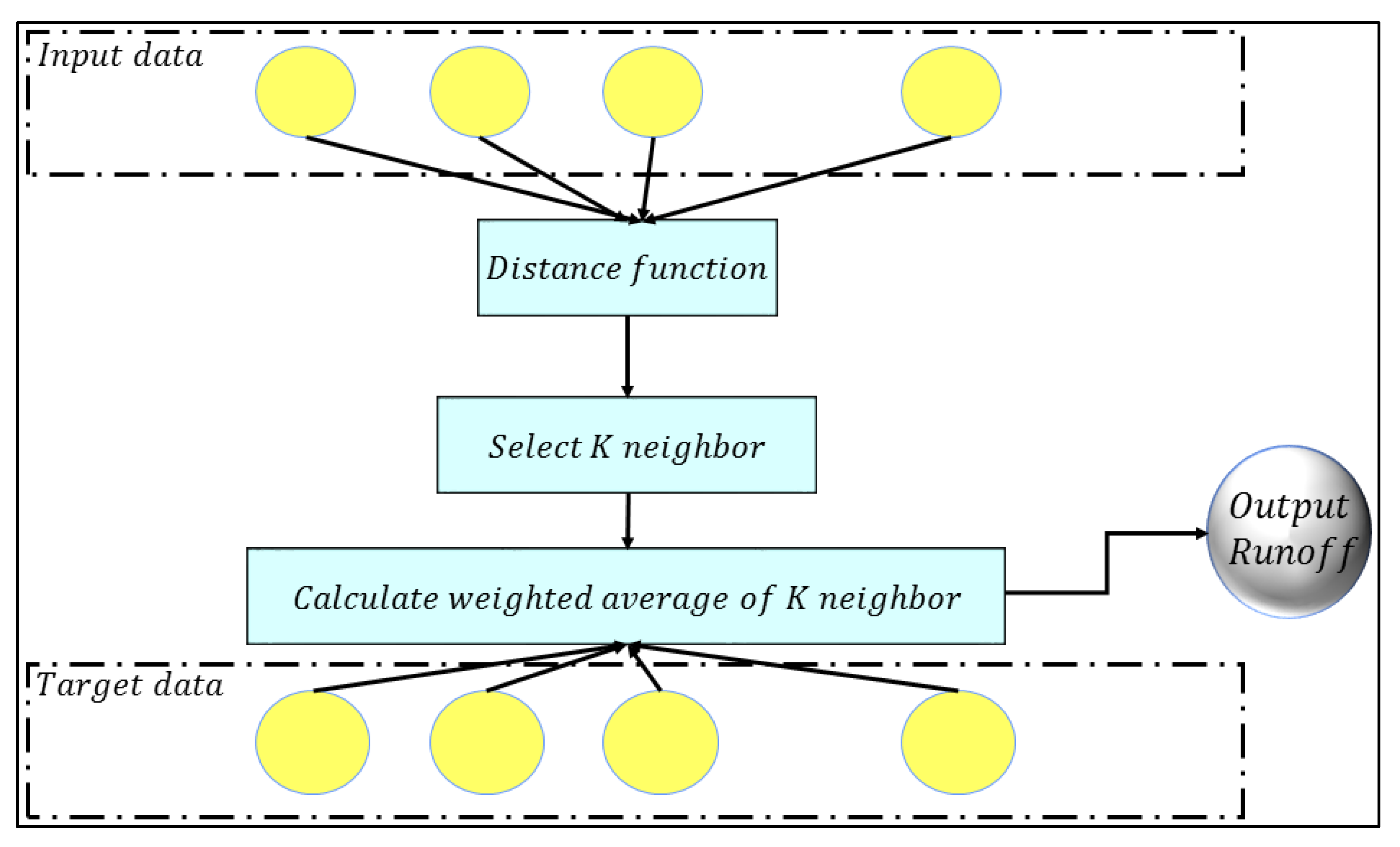
2.5. K-Nearest Neighbor (KNN)
2.6. Multivariate Adaptive Regression Spline (MARS)
2.7. M5 Model Tree (M5)
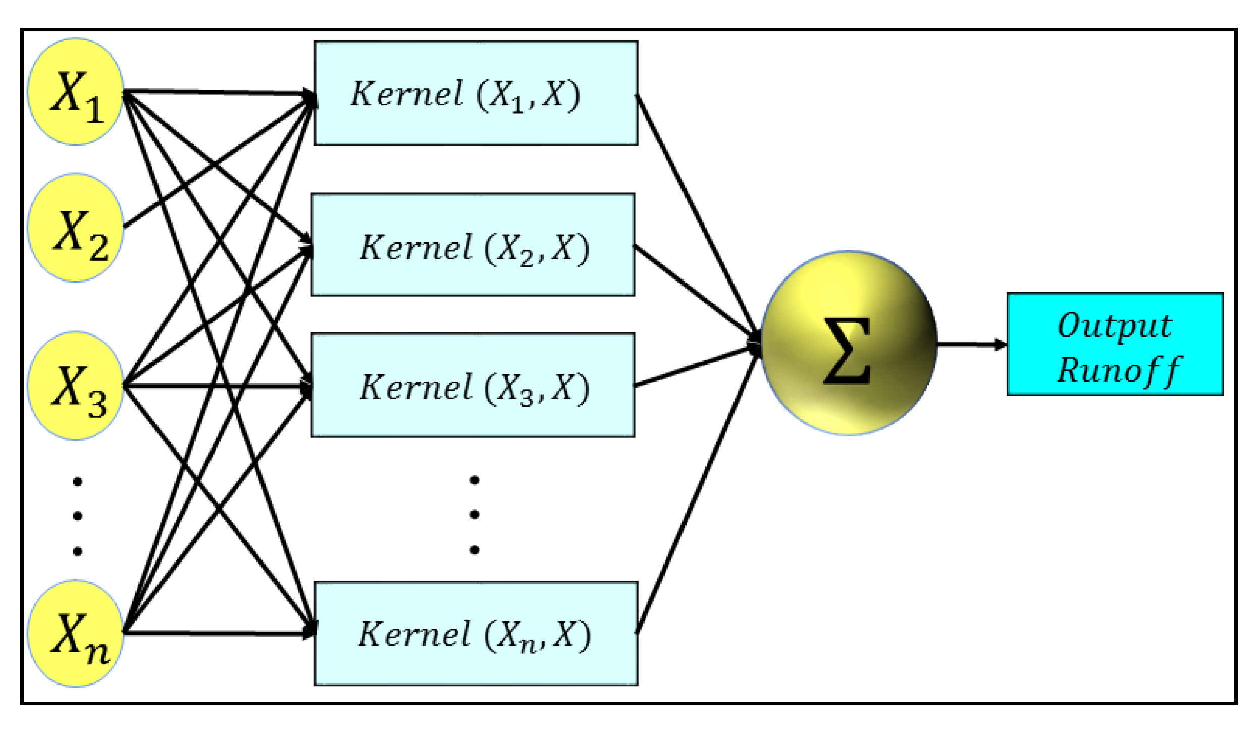
2.8. Least Square Support Vector Machine (LSSVM)
2.9. Random Forest Regression (RF)
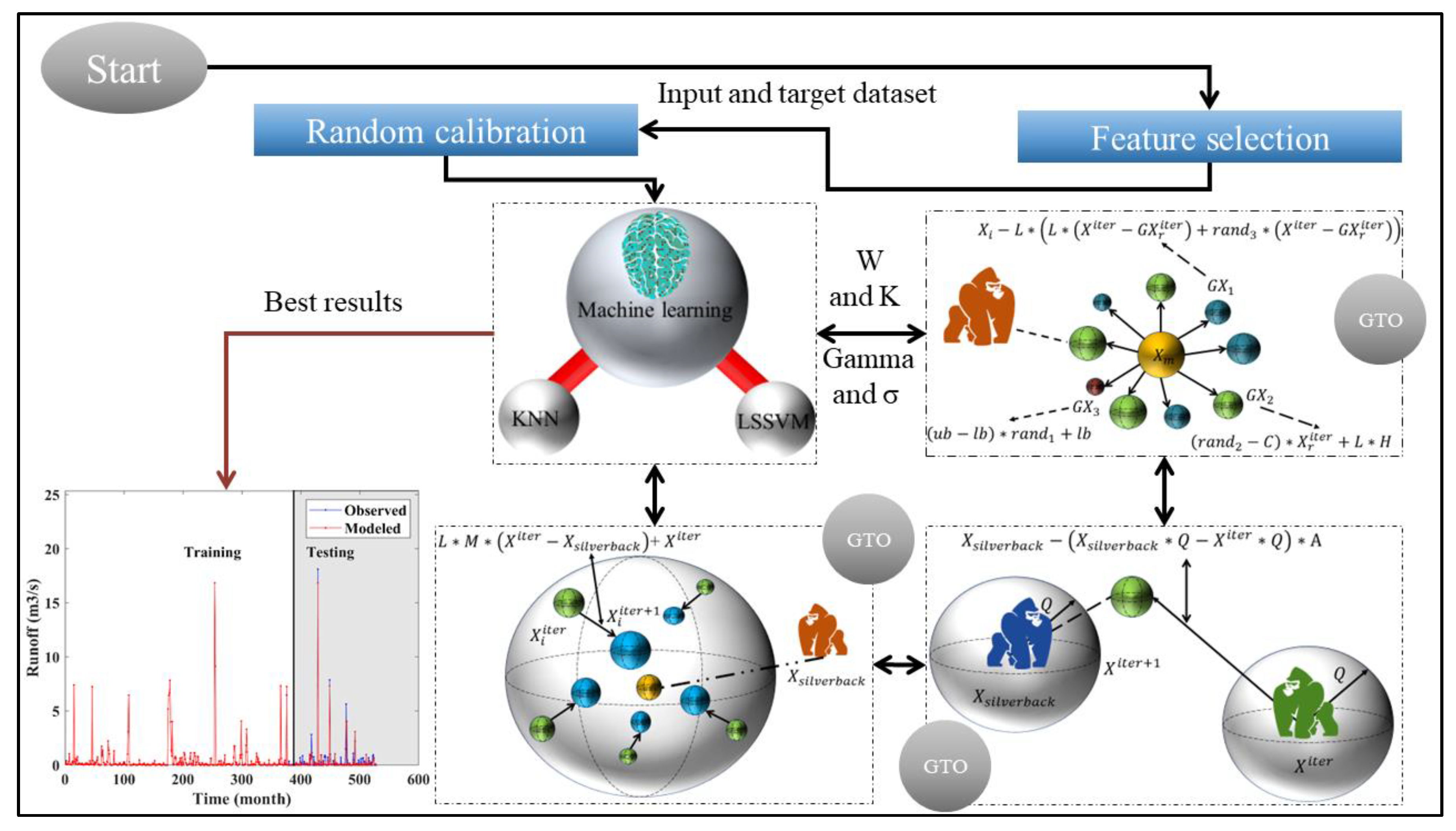
2.10. Gorilla Troop Optimizer (GTO)
2.11. Hybrid of LSSVM and KNN with Gorilla Troop Optimizer
| Algorithm 1. KNN–GTO and LSSVM–GTO |
| 1: Initialize parameters of GTO 2: Load inputs and target variables dataset 3: Generate the initial population of GTO 4: Train and test KNN and LSSVM for each artificial gorilla 5: Calculate the fitness function (MSE) for each artificial gorilla 6: iter: =1 7: while iter < Max_Iter do 8: Update the position of an artificial gorilla using Equations (10)–(19) 9: iter: = iter + 1 10: end while 11: Return the best solution (optimal W and K for KNN, and gamma and σ for LSSVM) |
2.12. Assessment Criteria
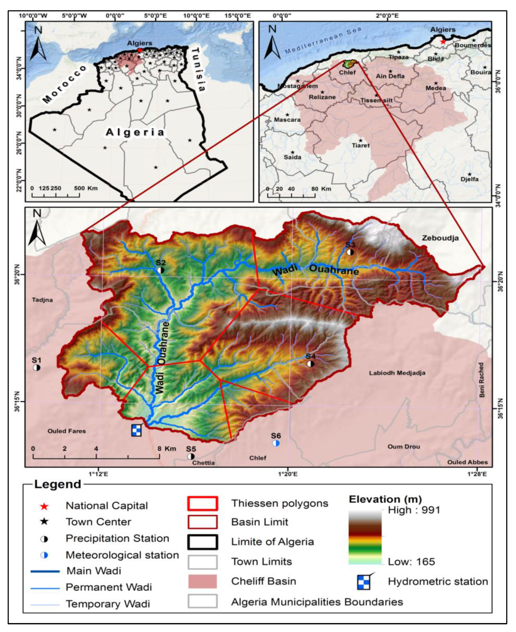
3. Case Study and Data Description
4. Presented Framework for Modeling Rainfall–Runoff
| Algorithm 2 feature selection |
| 1: Load input data and target data 2: Apply lag times to input data 3: while i < number of input features do 4: Calculate the Pearson correlation coefficient (R) between the feature and target data. 5: If R < threshold of R 6: Remove feature from the input data 7: end if 8: i: = i + 1 9: end while 10: Apply PCA to the remaining input data 11: Return the final inputs list |
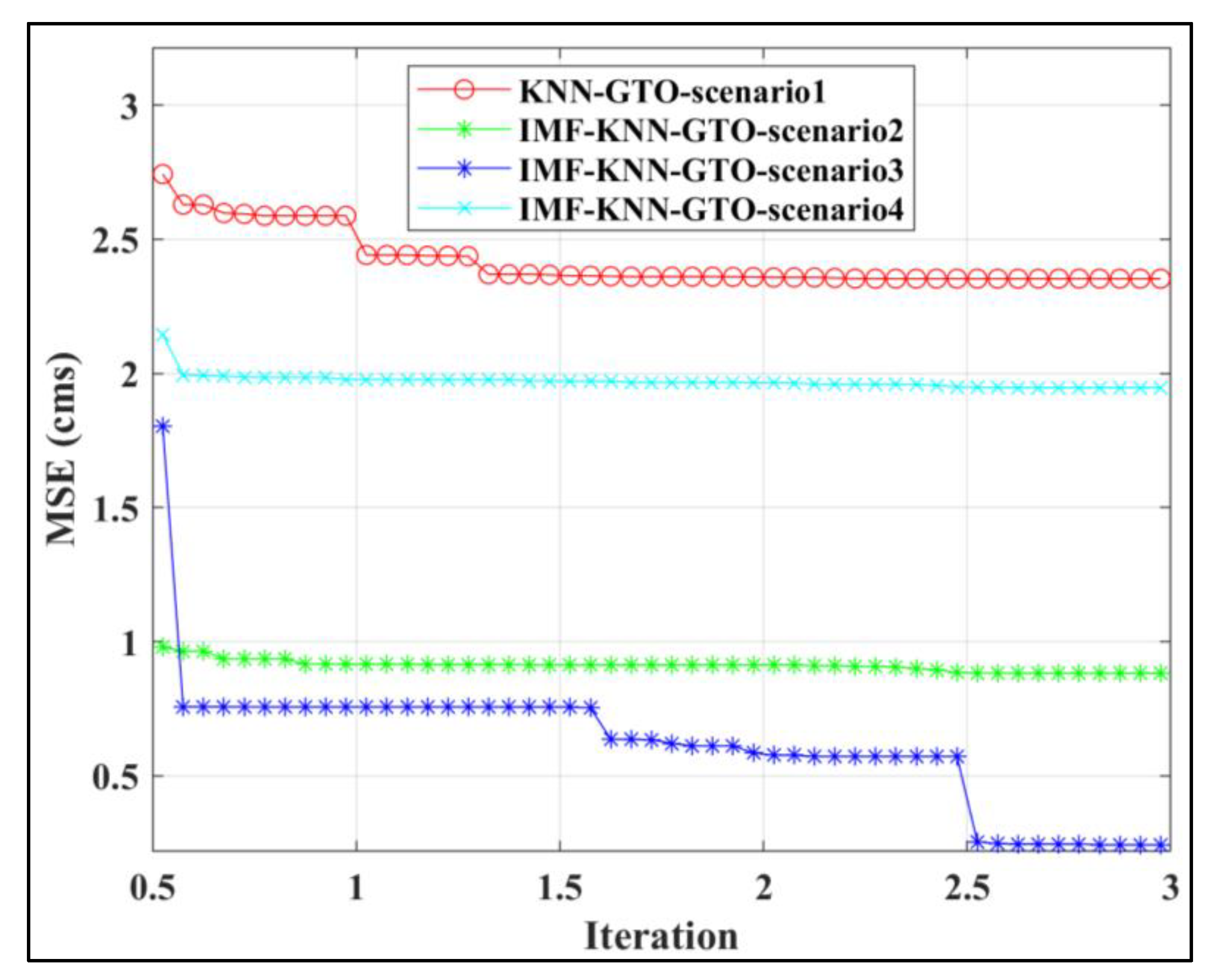
5. Results and Discussion
6. Conclusions
Author Contributions
Funding
Data Availability Statement
Acknowledgments
Conflicts of Interest
References
- Khan, M.T.; Shoaib, M.; Hammad, M.; Salahudin, H.; Ahmad, F.; Ahmad, S. Application of Machine Learning Techniques in Rainfall–Runoff Modelling of the Soan River Basin, Pakistan. Water 2021, 13, 3528. [Google Scholar] [CrossRef]
- Bhusal, A.; Parajuli, U.; Regmi, S.; Kalra, A. Application of Machine Learning and Process-Based Models for Rainfall-Runoff Simulation in Dupage River Basin, Illinois. Hydrology 2022, 9, 117. [Google Scholar] [CrossRef]
- Clark, M.P.; Kavetski, D.; Fenicia, F. Pursuing the Method of Multiple Working Hypotheses for Hydrological Modeling. Water Resour. Res. 2011, 47, W09301. [Google Scholar] [CrossRef]
- Niu, W.; Feng, Z.; Zeng, M.; Feng, B.; Min, Y.; Cheng, C.; Zhou, J. Forecasting Reservoir Monthly Runoff via Ensemble Empirical Mode Decomposition and Extreme Learning Machine Optimized by an Improved Gravitational Search Algorithm. Appl. Soft Comput. 2019, 82, 105589. [Google Scholar] [CrossRef]
- Li, H.; Zhang, Y.; Zhou, X. Predicting Surface Runoff from Catchment to Large Region. Adv. Meteorol. 2015, 2015, 1–13. [Google Scholar] [CrossRef]
- Song, X.; Kong, F.; Zhan, C.; Han, J. Hybrid Optimization Rainfall-Runoff Simulation Based on Xinanjiang Model and Artificial Neural Network. J. Hydrol. Eng. 2012, 17, 1033–1041. [Google Scholar] [CrossRef]
- Vafakhah, M.; Janizadeh, S. Application of Artificial Neural Network and Adaptive Neuro-Fuzzy Inference System in Streamflow Forecasting. In Advances in Streamflow Forecasting; Elsevier: Amsterdam, The Netherlands, 2021; pp. 171–191. [Google Scholar]
- Liu, Z.; Todini, E. Towards a Comprehensive Physically-Based Rainfall-Runoff Model. Hydrol. Earth Syst. Sci. 2002, 6, 859–881. [Google Scholar] [CrossRef]
- Xu, C.-Y.; Xiong, L.; Singh, V.P. Black-Box Hydrological Models. In Handbook of Hydrometeorological Ensemble Forecasting; Springer: Berlin/Heidelberg, Germany, 2017; pp. 1–48. [Google Scholar]
- Seo, Y.; Kim, S.; Singh, V.P. Machine Learning Models Coupled with Variational Mode Decomposition: A New Approach for Modeling Daily Rainfall-Runoff. Atmosphere 2018, 9, 251. [Google Scholar] [CrossRef]
- Mohammadi, B. A Review on the Applications of Machine Learning for Runoff Modeling. Sustain. Water Resour. Manag. 2021, 7, 98. [Google Scholar]
- Nourani, V.; Gökçekuş, H.; Gichamo, T. Ensemble Data-Driven Rainfall-Runoff Modeling Using Multi-Source Satellite and Gauge Rainfall Data Input Fusion. Earth Sci. Inform. 2021, 14, 1787–1808. [Google Scholar] [CrossRef]
- Sharafati, A.; Khazaei, M.R.; Nashwan, M.S.; Al-Ansari, N.; Yaseen, Z.M.; Shahid, S. Assessing the Uncertainty Associated with Flood Features Due to Variability of Rainfall and Hydrological Parameters. Adv. Civ. Eng. 2020, 2020, 1–9. [Google Scholar] [CrossRef]
- Mohammadi, B.; Guan, Y.; Moazenzadeh, R.; Safari, M.J.S. Implementation of Hybrid Particle Swarm Optimization-Differential Evolution Algorithms Coupled with Multi-Layer Perceptron for Suspended Sediment Load Estimation. CATENA 2021, 198, 105024. [Google Scholar] [CrossRef]
- Tikhamarine, Y.; Souag-Gamane, D.; Ahmed, A.N.; Sammen, S.S.; Kisi, O.; Huang, Y.F.; El-Shafie, A. Rainfall-Runoff Modelling Using Improved Machine Learning Methods: Harris Hawks Optimizer vs. Particle Swarm Optimization. J. Hydrol. 2020, 589, 125133. [Google Scholar] [CrossRef]
- Adnan, R.M.; Petroselli, A.; Heddam, S.; Santos, C.A.G.; Kisi, O. Short Term Rainfall-Runoff Modelling Using Several Machine Learning Methods and a Conceptual Event-Based Model. Stoch. Environ. Res. Risk Assess. 2021, 35, 597–616. [Google Scholar] [CrossRef]
- Okkan, U.; Ersoy, Z.B.; Kumanlioglu, A.A.; Fistikoglu, O. Embedding Machine Learning Techniques into a Conceptual Model to Improve Monthly Runoff Simulation: A Nested Hybrid Rainfall-Runoff Modeling. J. Hydrol. 2021, 598, 126433. [Google Scholar] [CrossRef]
- Roy, B.; Singh, M.P.; Kaloop, M.R.; Kumar, D.; Hu, J.-W.; Kumar, R.; Hwang, W.-S. Data-Driven Approach for Rainfall-Runoff Modelling Using Equilibrium Optimizer Coupled Extreme Learning Machine and Deep Neural Network. Appl. Sci. 2021, 11, 6238. [Google Scholar] [CrossRef]
- Waqas, M.; Saifullah, M.; Hashim, S.; Khan, M.; Muhammad, S. Evaluating the Performance of Different Artificial Intelligence Techniques for Forecasting: Rainfall and Runoff Prospective. In Weather Forecast; IntechOpen: London, UK, 2021; p. 23. [Google Scholar]
- Xiao, L.; Zhong, M.; Zha, D. Runoff Forecasting Using Machine-Learning Methods: Case Study in the Middle Reaches of Xijiang River. Front. Big Data 2022, 4, 752406. [Google Scholar] [CrossRef]
- Singh, A.K.; Kumar, P.; Ali, R.; Al-Ansari, N.; Vishwakarma, D.K.; Kushwaha, K.S.; Panda, K.C.; Sagar, A.; Mirzania, E.; Elbeltagi, A. Application of Machine Learning Technique for Rainfall-Runoff Modelling of Highly Dynamic Watersheds. arXiv 2022. [Google Scholar] [CrossRef]
- Yang, M.-C.; Wang, J.-Z.; Sun, T.-Y. EMD-Based Preprocessing with a Fuzzy Inference System and a Fuzzy Neural Network to Identify Kiln Coating Collapse for Predicting Refractory Failure in the Cement Process. Int. J. Fuzzy Syst. 2018, 20, 2640–2656. [Google Scholar] [CrossRef]
- Rouillard, V.; Sek, M.A. The Use of Intrinsic Mode Functions to Characterize Shock and Vibration in the Distribution Environment. Packag. Technol. Sci. 2005, 18, 39–51. [Google Scholar] [CrossRef]
- Khorsandi, M.; Ashofteh, P.-S.; Azadi, F.; Chu, X. Multi-Objective Firefly Integration with the K-Nearest Neighbor to Reduce Simulation Model Calls to Accelerate the Optimal Operation of Multi-Objective Reservoirs. Water Resour. Manag. 2022, 36, 3283–3304. [Google Scholar] [CrossRef]
- Guijo-Rubio, D.; Gutiérrez, P.A.; Casanova-Mateo, C.; Fernández, J.C.; Gómez-Orellana, A.M.; Salvador-González, P.; Salcedo-Sanz, S.; Hervás-Martínez, C. Prediction of Convective Clouds Formation Using Evolutionary Neural Computation Techniques. Neural Comput. Appl. 2020, 32, 13917–13929. [Google Scholar] [CrossRef]
- Mohaghegh, A.; Farzin, S.; Anaraki, M.V. A New Framework for Missing Data Estimation and Reconstruction Based on the Geographical Input Information, Data Mining, and Multi-Criteria Decision-Making; Theory and Application in Missing Groundwater Data of Damghan Plain, Iran. Groundw. Sustain. Dev. 2022, 17, 100767. [Google Scholar] [CrossRef]
- Chen, Y.; Chen, R.; Ma, C.; Tan, P. Short-Term Wind Speeds Prediction of SVM Based on Simulated Annealing Algorithm with Gauss Perturbation. IOP Conf. Ser. Earth Environ. Sci. 2019, 267, 042032. [Google Scholar] [CrossRef]
- Breiman, L. Random Forests. Mach. Learn 2001, 45, 5–32. [Google Scholar] [CrossRef]
- Ginidi, A.; Ghoneim, S.M.; Elsayed, A.; El-Sehiemy, R.; Shaheen, A.; El-Fergany, A. Gorilla Troops Optimizer for Electrically Based Single and Double-Diode Models of Solar Photovoltaic Systems. Sustainability 2021, 13, 9459. [Google Scholar] [CrossRef]
- Pachpore, S.; Jadhav, P.; Ghorpade, R. Process Parameter Optimization in Manufacturing of Root Canal Device Using Gorilla Troops Optimization Algorithm. In Computational Intelligence in Manufacturing; Elsevier: Amsterdam, The Netherlands, 2022; pp. 175–185. [Google Scholar]
- Daneshfaraz, R.; Aminvash, E.; Ghaderi, A.; Abraham, J.; Bagherzadeh, M. SVM Performance for Predicting the Effect of Horizontal Screen Diameters on the Hydraulic Parameters of a Vertical Drop. Appl. Sci. 2021, 11, 4238. [Google Scholar] [CrossRef]
- Morshed-Bozorgdel, A.; Kadkhodazadeh, M.; Valikhan Anaraki, M.; Farzin, S. A Novel Framework Based on the Stacking Ensemble Machine Learning (SEML) Method: Application in Wind Speed Modeling. Atmosphere 2022, 13, 758. [Google Scholar] [CrossRef]
- De Salis, H.H.C.; da Costa, A.M.; Vianna, J.H.M.; Schuler, M.A.; Künne, A.; Fernandes, L.F.S.; Pacheco, F.A.L. Hydrologic Modeling for Sustainable Water Resources Management in Urbanized Karst Areas. Int. J. Environ. Res. Public Health 2019, 16, 2542. [Google Scholar] [CrossRef]
- Anaraki, M.V.; Farzin, S.; Mousavi, S.-F.; Karami, H. Uncertainty Analysis of Climate Change Impacts on Flood Frequency by Using Hybrid Machine Learning Methods. Water Resour. Manag. 2021, 35, 199–223. [Google Scholar] [CrossRef]
- Jamei, M.; Ali, M.; Malik, A.; Prasad, R.; Abdulla, S.; Yaseen, Z.M. Forecasting Daily Flood Water Level Using Hybrid Advanced Machine Learning Based Time-Varying Filtered Empirical Mode Decomposition Approach. Water Resour. Manag. 2022, 36, 4637–4676. [Google Scholar] [CrossRef]
- Zhou, R.; Zhang, Y. Reconstruction of Missing Spring Discharge by Using Deep Learning Models with Ensemble Empirical Mode Decomposition of Precipitation. Environ. Sci. Pollut. Res. 2022, 29, 82451–82466. [Google Scholar] [CrossRef] [PubMed]


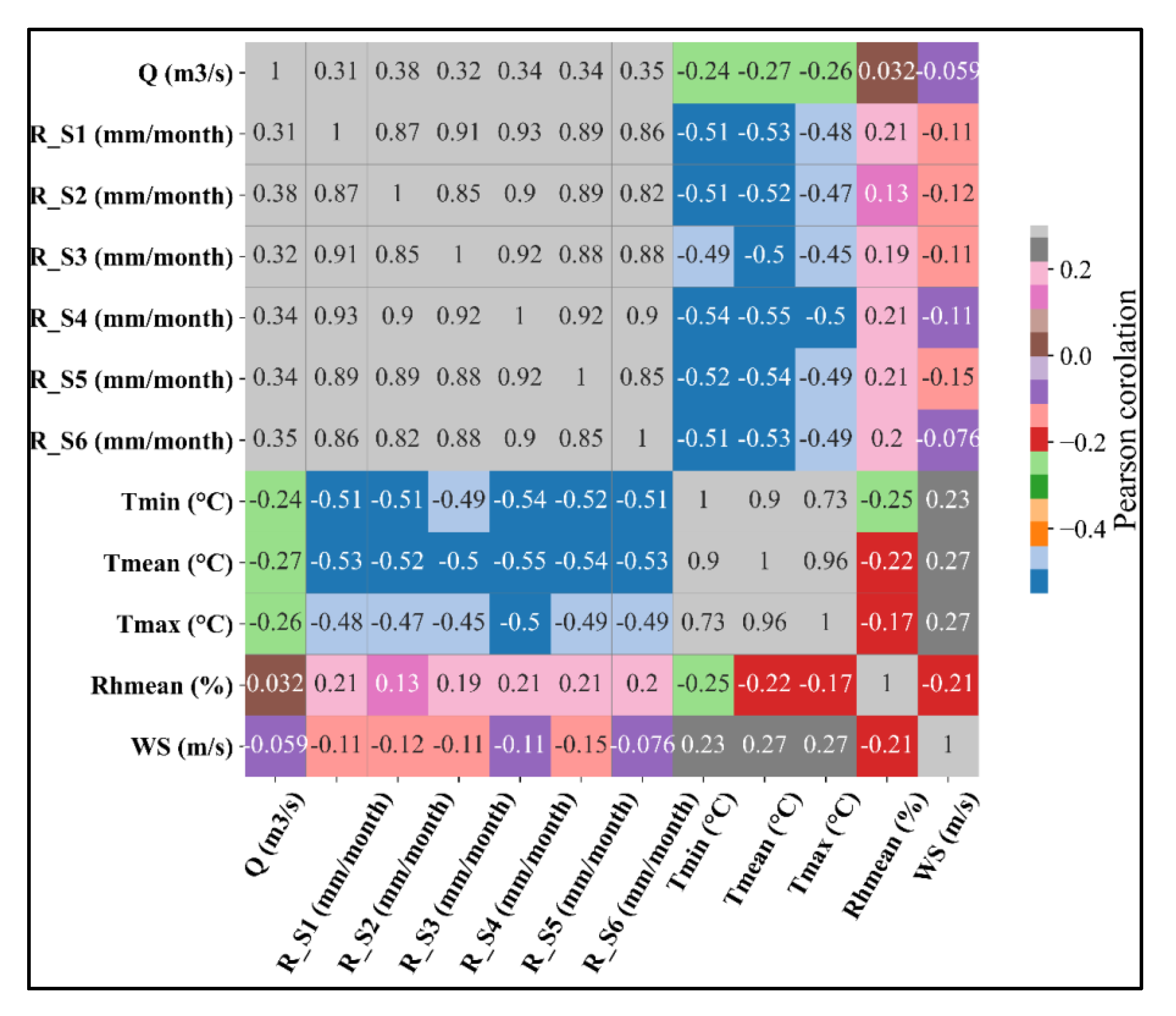
| Statistics | Q (m3/s) | S1 | S2 | S3 | S4 | S5 | S6 | Tmin (°C) | Tmean (°C) | Tmax (°C) | RHmean (%) | WS (m/s) |
|---|---|---|---|---|---|---|---|---|---|---|---|---|
| Rainfall (mm/Month) | ||||||||||||
| Mean | 0.47 | 30.29 | 40.57 | 27.81 | 32.48 | 35.44 | 33.96 | 12.34 | 25.8 | 28.01 | 50.38 | 2.58 |
| Standard deviation | 1.54 | 32.15 | 48.01 | 30.3 | 34.2 | 38.44 | 34.63 | 6.09 | 7.07 | 9.2 | 26.63 | 0.71 |
| Minimum | 0 | 0 | 0 | 0 | 0 | 0 | 0 | −1.5 | 0 | 0 | 0 | 0.6 |
| Maximum | 18.1 | 167.6 | 336.4 | 156.3 | 175.05 | 265.2 | 172.3 | 24.7 | 51.83 | 96.27 | 82.5 | 4.9 |
| Coefficient of variation | 0.31 | 0.94 | 0.85 | 0.92 | 0.95 | 0.92 | 0.98 | 2.03 | 2.69 | 2.8 | 1.89 | 3.63 |
| Skewness coefficient | 6.82 | 1.28 | 1.81 | 1.42 | 1.29 | 1.72 | 1.23 | 0.17 | 0.36 | 0.92 | −1.09 | −0.12 |
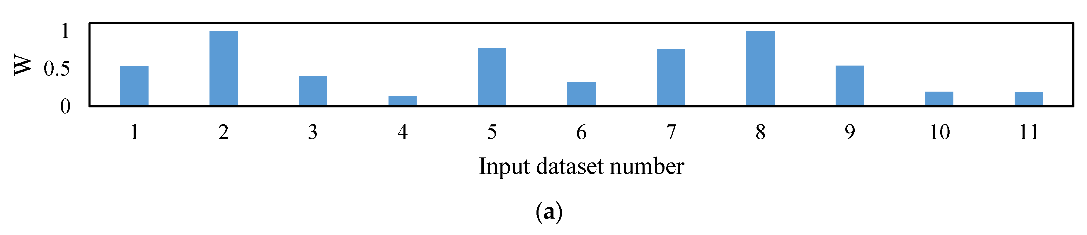
| Scenarios | Inputs | Threshold of R | Pre-Processing | Post-Processing |
|---|---|---|---|---|
| 1 | R_1, R_2, R_3, R_4, R_5, R_6, Tmin, Tmean, Tmax, Rh_mean, SW | - | - | - |
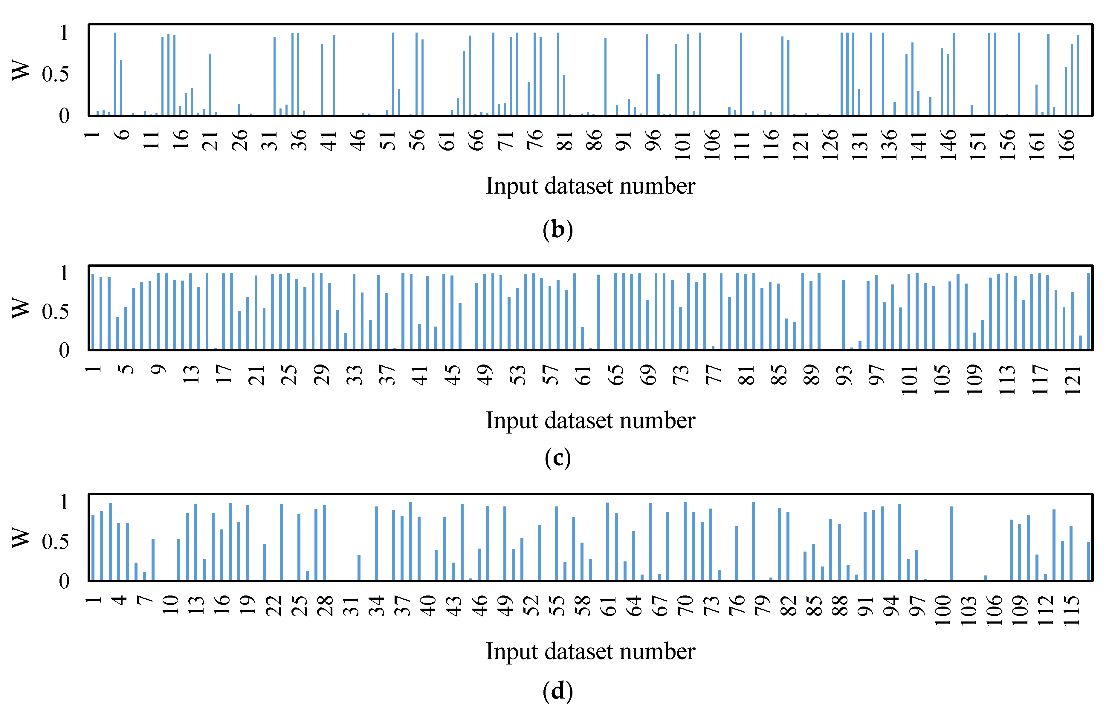
| 2 | R_1, R_2, R_3, R_4, R_5, R_6, Tmin, Tmean, Tmax, Rh_mean, SW Lag = 0:24 month | 0.05 | - | - |
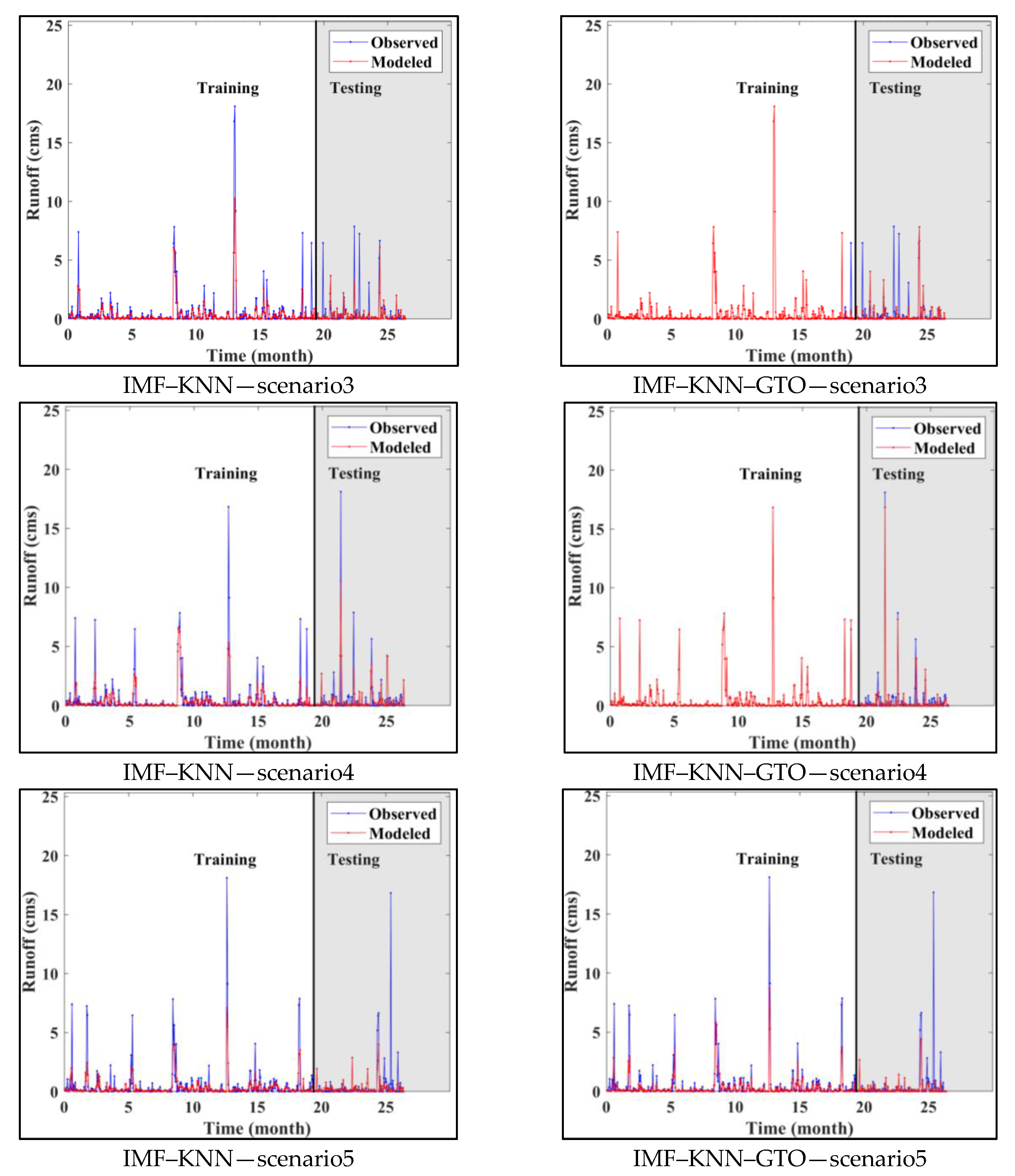
| 3 | R_1, R_2, R_3, R_4, R_5, R_6, Tmin, Tmean, Tmax, Rh_mean, SW Lag = 0:24 month | 0.1 | IMF (MaxNumIMF = 3) | PCA |
| 4 | R_1, R_2, R_3, R_4, R_5, R_6, Tmin, Tmean, Tmax, Rh_mean, SW Lag = 0:24 month | 0.1 | IMF (MaxNumIMF = 4) | PCA |
| 5 | R_1, R_2, R_3, R_4, R_5, R_6, Tmin, Tmean, Tmax, Rh_mean, SW Lag = 0:24 month | 0.1 | IMF (MaxNumIMF = 5) | PCA |
| Scenarios | Algorithm | N1/N2 | γ/σ | minLSize/sThreshold | mF/C | NumTree | K |
|---|---|---|---|---|---|---|---|
| 1 | ANN | 1/5 | - | - | - | - | - |
| LSSVM | - | 4.90/6.00 | - | - | - | - | |
| M5 | - | - | 64/0.01 | - | - | - | |
| MARS | - | - | - | 5/4 | - | - | |
| RF | - | - | 4/0.05 | - | 100 | - | |
| LSSVM–GTO | - | 5.23/6.19 | - | - | - | - | |
| KNN | - | - | - | - | - | 13 | |
| KNN–GTO | - | - | - | - | - | 4 | |
| 2 | ANN | 15/4 | - | - | - | - | - |
| LSSVM | - | 10/5 | - | - | - | - | |
| M5 | - | - | 64/0.01 | - | - | - | |
| MARS | - | - | - | 5/4 | - | - | |
| RF | - | - | 8/0.01 | - | 100 | - | |
| LSSVM–GTO | - | 100/8.16 | - | - | - | - | |
| KNN | - | - | - | - | - | 2 | |
| KNN–GTO | - | - | - | - | - | 2 | |
| 3 | ANN | 10/7 | - | - | - | - | - |
| LSSVM | - | 10/5 | - | - | - | - | |
| M5 | - | - | 64/0.01 | - | - | - | |
| MARS | - | - | - | 5/4 | - | - | |
| RF | - | - | 32/0.1 | - | 100 | - | |
| LSSVM–GTO | - | 100/7.43 | - | - | - | - | |
| KNN | - | - | - | - | - | 3 | |
| KNN–GTO | - | - | - | - | - | 1 | |
| 4 | ANN | 12/4 | - | - | - | - | - |
| LSSVM | - | 10/5 | - | - | - | - | |
| M5 | - | - | 64/0.1 | - | - | - | |
| MARS | - | - | - | 30/6 | - | - | |
| RF | - | - | 32/0.01 | - | 100 | - | |
| LSSVM–GTO | - | 1.38/2.33 | - | - | - | - | |
| KNN | - | - | - | - | - | 4 | |
| KNN–GTO | - | - | - | - | - | 1 | |
| 5 | ANN | 7/7 | - | - | - | - | - |
| LSSVM | - | 10/5 | - | - | - | - | |
| M5 | - | - | 64/0.1 | - | - | - | |
| MARS | - | - | - | 30/4 | - | - | |
| RF | - | - | 8/0.01 | - | 100 | - | |
| LSSVM–GTO | - | 100/8.35 | - | - | - | - | |
| KNN | - | - | - | - | - | 5 | |
| KNN–GTO | - | - | - | - | - | 4 |
| Scenarios | Algorithm | MAE | RMSE | RRMSE | R | NSE | KGE |
|---|---|---|---|---|---|---|---|
| 1 | ANN | 0.4540 | 1.3057 | 0.9052 | 0.4608 | 0.1786 | −0.1042 |
| LSSVM | 0.3175 | 0.7779 | 0.7240 | 0.7135 | 0.4745 | 0.3187 | |
| M5 | 0.5356 | 1.4645 | 0.8855 | 0.4625 | 0.2139 | 0.0477 | |
| MARS | 0.5679 | 1.4487 | 0.8759 | 0.4804 | 0.2308 | 0.0717 | |
| RF | 0.3314 | 1.0234 | 0.6188 | 0.8354 | 0.6161 | 0.4567 | |
| MNLR | 0.4304 | 0.8965 | 0.8343 | 0.5497 | 0.3022 | 0.1695 | |
| LSSVM–GTO | 0.3174 | 0.7776 | 0.7237 | 0.7138 | 0.4749 | 0.3192 | |
| KNN | 0.5667 | 1.6160 | 0.9238 | 0.4109 | 0.1444 | −0.1271 | |
| KNN–GTO | 0.5364 | 1.6365 | 0.9355 | 0.4277 | 0.1226 | −0.1896 | |
| 2 | ANN | 0.0209 | 0.0446 | 0.0345 | 0.9996 | 0.9988 | 0.9749 |
| LSSVM | 0.1582 | 0.4317 | 0.3266 | 0.9827 | 0.8931 | 0.7108 | |
| M5 | 0.4137 | 0.9160 | 0.7525 | 0.6574 | 0.4322 | 0.3368 | |
| MARS | 0.3545 | 0.8260 | 0.6380 | 0.7693 | 0.5918 | 0.5312 | |
| RF | 0.1968 | 0.7060 | 0.4956 | 0.9085 | 0.7537 | 0.6003 | |
| MNLR | 0.4526 | 0.6950 | 0.5709 | 0.8205 | 0.6731 | 0.6271 | |
| LSSVM–GTO | 0.0703 | 0.1859 | 0.1406 | 0.9972 | 0.9802 | 0.8773 | |
| KNN | 0.2498 | 0.8191 | 0.5750 | 0.8207 | 0.6685 | 0.5678 | |
| KNN–GTO | 0.0013 | 0.0127 | 0.0089 | 1.0000 | 0.9999 | 0.9969 | |
| 3 | ANN | 0.0000 | 0.0000 | 0.0000 | 1.0000 | 1.0000 | 1.0000 |
| LSSVM | 0.1268 | 0.3296 | 0.2015 | 0.9941 | 0.9593 | 0.8232 | |
| M5 | 0.1856 | 0.7773 | 0.4796 | 0.8771 | 0.7694 | 0.7387 | |
| MARS | 0.4922 | 1.0055 | 0.8394 | 0.5418 | 0.2935 | 0.1580 | |
| RF | 0.2838 | 0.8688 | 0.5312 | 0.9236 | 0.7171 | 0.5305 | |
| MNLR | 0.4343 | 0.6578 | 0.5491 | 0.8353 | 0.6977 | 0.6557 | |
| LSSVM–GTO | 0.0529 | 0.1304 | 0.0797 | 0.9989 | 0.9936 | 0.9344 | |
| KNN | 0.3353 | 0.9785 | 0.5865 | 0.8206 | 0.6551 | 0.5454 | |
| KNN–GTO | 0.2839 | 0.8923 | 0.5348 | 0.8631 | 0.7132 | 0.5837 | |
| 4 | ANN | 0.0277 | 0.0440 | 0.0300 | 0.9996 | 0.9991 | 0.9892 |
| LSSVM | 0.1688 | 0.4213 | 0.2811 | 0.9874 | 0.9208 | 0.7525 | |
| M5 | 0.3262 | 0.9896 | 0.6500 | 0.7592 | 0.5764 | 0.5127 | |
| MARS | 0.4541 | 0.7097 | 0.4662 | 0.8844 | 0.7821 | 0.7533 | |
| RF | 0.2547 | 0.8613 | 0.5068 | 0.9040 | 0.7424 | 0.5878 | |
| MNLR | 0.5617 | 0.9386 | 0.6262 | 0.7790 | 0.6068 | 0.5489 | |
| LSSVM–GTO | 0.0628 | 0.1525 | 0.1001 | 0.9981 | 0.9899 | 0.9184 | |
| KNN | 0.3389 | 0.9946 | 0.6533 | 0.7579 | 0.5721 | 0.4838 | |
| KNN–GTO | 0.0001 | 0.0016 | 0.0011 | 1.0000 | 1.0000 | 0.9998 | |
| 5 | ANN | 0.0405 | 0.0693 | 0.0403 | 0.9994 | 0.9984 | 0.9498 |
| LSSVM | 0.1523 | 0.3627 | 0.2499 | 0.9908 | 0.9374 | 0.7790 | |
| M5 | 0.0795 | 0.4670 | 0.3217 | 0.9467 | 0.8962 | 0.8833 | |
| MARS | 0.5338 | 1.1197 | 0.6983 | 0.7149 | 0.5111 | 0.4340 | |
| RF | 0.2694 | 0.8038 | 0.4673 | 0.9604 | 0.7810 | 0.5769 | |
| MNLR | 0.4770 | 0.7890 | 0.5436 | 0.8389 | 0.7037 | 0.6627 | |
| LSSVM–GTO | 0.0588 | 0.1302 | 0.0897 | 0.9986 | 0.9919 | 0.9252 | |
| KNN | 0.2279 | 0.8323 | 0.4819 | 0.8875 | 0.7671 | 0.6455 | |
| KNN–GTO | 0.0001 | 0.0021 | 0.0012 | 1.0000 | 1.0000 | 0.9998 |
| Scenarios | Algorithm | MAE | RMSE | RRMSE | R | NSE | KGE | Friedman Ranking |
|---|---|---|---|---|---|---|---|---|
| 1 | ANN | 0.4827 | 1.5902 | 0.9017 | 0.4684 | 0.1820 | −0.1069 | 35.3333 |
| LSSVM | 0.7111 | 2.1998 | 0.9625 | 0.2941 | 0.0679 | −0.2475 | 45.3333 | |
| M5 | 0.5516 | 1.1938 | 0.9569 | 0.4099 | 0.0787 | 0.0760 | 35.6667 | |
| MARS | 0.5333 | 1.1759 | 0.9426 | 0.4172 | 0.1061 | 0.1119 | 33.3333 | |
| RF | 0.5239 | 1.2307 | 0.9865 | 0.3974 | 0.0208 | 0.1007 | 36.6667 | |
| MNLR | 0.8219 | 2.2490 | 0.9840 | 0.2186 | 0.0257 | −0.2600 | 48.8333 | |
| LSSVM–GTO | 0.7111 | 2.1998 | 0.9625 | 0.2940 | 0.0679 | −0.2474 | 45.3333 | |
| KNN | 0.3545 | 0.7886 | 0.9072 | 0.4470 | 0.1720 | 0.0744 | 27.6667 | |
| KNN–GTO | 0.3156 | 0.7537 | 0.8671 | 0.5006 | 0.2435 | 0.0502 | 24.8333 | |
| 2 | ANN | 0.6039 | 1.8606 | 0.9227 | 0.4193 | 0.1432 | 0.0838 | 39.3333 |
| LSSVM | 0.5587 | 1.6312 | 0.8277 | 0.6487 | 0.3105 | 0.0923 | 29.6667 | |
| M5 | 0.4699 | 1.6769 | 0.7885 | 0.6787 | 0.3743 | 0.1388 | 23.3333 | |
| MARS | 0.4682 | 1.5109 | 0.7493 | 0.6625 | 0.4350 | 0.3069 | 17.8333 | |
| RF | 0.4893 | 1.5880 | 0.8834 | 0.4788 | 0.2147 | −0.0066 | 34.0000 | |
| MNLR | 0.7810 | 1.7083 | 0.8033 | 0.5944 | 0.3507 | 0.1959 | 31.0000 | |
| LSSVM–GTO | 0.5491 | 1.5716 | 0.7975 | 0.6690 | 0.3599 | 0.1570 | 24.3333 | |
| KNN | 0.4925 | 1.6548 | 0.9205 | 0.4460 | 0.1472 | −0.2137 | 37.5000 | |
| KNN–GTO | 0.3823 | 1.5340 | 0.8534 | 0.5365 | 0.2671 | 0.0273 | 29.6667 | |
| 3 | ANN | 0.5885 | 1.1976 | 0.6946 | 0.7428 | 0.5144 | 0.5419 | 13.1667 |
| LSSVM | 0.4661 | 0.9855 | 0.7543 | 0.6998 | 0.4274 | 0.2388 | 14.8333 | |
| M5 | 0.4572 | 1.2876 | 0.9547 | 0.3579 | 0.0827 | −0.1658 | 35.1667 | |
| MARS | 0.5875 | 1.6682 | 0.7769 | 0.6411 | 0.3925 | 0.3570 | 22.6667 | |
| RF | 0.5245 | 1.1745 | 0.8989 | 0.4489 | 0.1869 | −0.0441 | 33.0000 | |
| MNLR | 0.7334 | 1.6685 | 0.7771 | 0.6350 | 0.3922 | 0.2339 | 26.3333 | |
| LSSVM–GTO | 0.4675 | 0.9404 | 0.7197 | 0.7167 | 0.4787 | 0.2911 | 13.0000 | |
| KNN | 0.2897 | 0.7242 | 0.6031 | 0.8053 | 0.6340 | 0.5264 | 5.0000 | |
| KNN–GTO | 0.2354 | 0.6521 | 0.5431 | 0.8746 | 0.7032 | 0.5316 | 3.1667 | |
| 4 | ANN | 0.4257 | 1.2139 | 0.7069 | 0.7414 | 0.4971 | 0.5129 | 10.5000 |
| LSSVM | 0.4576 | 1.3281 | 0.8070 | 0.6323 | 0.3446 | 0.1247 | 23.0000 | |
| M5 | 0.5240 | 1.5408 | 0.9678 | 0.3241 | 0.0574 | −0.0401 | 40.1667 | |
| MARS | 0.5581 | 1.0767 | 0.6763 | 0.7356 | 0.5397 | 0.4471 | 12.5000 | |
| RF | 0.4124 | 0.8672 | 0.7951 | 0.6471 | 0.3638 | 0.1145 | 17.8333 | |
| MNLR | 0.6971 | 1.1739 | 0.7133 | 0.7004 | 0.4880 | 0.4188 | 16.0000 | |
| LSSVM–GTO | 0.5097 | 1.2447 | 0.7818 | 0.6646 | 0.3849 | 0.0786 | 22.5000 | |
| KNN | 0.3052 | 0.9475 | 0.5951 | 0.8469 | 0.6436 | 0.4863 | 6.1667 | |
| KNN–GTO | 0.1640 | 0.4741 | 0.2978 | 0.9607 | 0.9108 | 0.7141 | 1.3333 | |
| 5 | ANN | 0.2895 | 0.7241 | 0.7124 | 0.7193 | 0.4892 | 0.3207 | 7.8333 |
| LSSVM | 0.4999 | 1.4501 | 0.8313 | 0.5962 | 0.3046 | 0.0991 | 28.1667 | |
| M5 | 0.4582 | 1.4096 | 0.8080 | 0.5973 | 0.3429 | 0.1317 | 23.8333 | |
| MARS | 0.7892 | 1.4660 | 1.0491 | 0.2993 | −0.1077 | 0.0406 | 43.8333 | |
| RF | 0.4198 | 0.8954 | 0.8810 | 0.4904 | 0.2190 | −0.0040 | 27.3333 | |
| MNLR | 0.7695 | 1.4628 | 0.8385 | 0.5659 | 0.2924 | 0.2631 | 30.3333 | |
| LSSVM–GTO | 0.4979 | 1.4151 | 0.8112 | 0.6039 | 0.3378 | 0.1526 | 25.1667 | |
| KNN | 0.3212 | 0.7952 | 0.8114 | 0.5972 | 0.3374 | 0.3034 | 18.3333 | |
| KNN–GTO | 0.1728 | 0.4016 | 0.4098 | 0.9162 | 0.8310 | 0.7187 | 1.6667 |
| ANN | LSSVM | M5 | MARS | RF | MNLR | LSSVM–GTO | KNN | KNN–GTO | |
|---|---|---|---|---|---|---|---|---|---|
| Training | −0.49 | 2.26 | 0.00 | 0.00 | 0.03 | 0.00 | 1.25 | −4.68 | 0.02 |
| Testing | 18.23 | 22.21 | 25.41 | 9.00 | 36.54 | −11.28 | 48.66 | −6.36 | −23.90 |
| All | 4.97 | 7.20 | 5.94 | 2.10 | 8.12 | −2.79 | 12.33 | −5.07 | −5.57 |
Disclaimer/Publisher’s Note: The statements, opinions and data contained in all publications are solely those of the individual author(s) and contributor(s) and not of MDPI and/or the editor(s). MDPI and/or the editor(s) disclaim responsibility for any injury to people or property resulting from any ideas, methods, instructions or products referred to in the content. |
© 2023 by the authors. Licensee MDPI, Basel, Switzerland. This article is an open access article distributed under the terms and conditions of the Creative Commons Attribution (CC BY) license (https://creativecommons.org/licenses/by/4.0/).
Share and Cite
Anaraki, M.V.; Achite, M.; Farzin, S.; Elshaboury, N.; Al-Ansari, N.; Elkhrachy, I. Modeling of Monthly Rainfall–Runoff Using Various Machine Learning Techniques in Wadi Ouahrane Basin, Algeria. Water 2023, 15, 3576. https://doi.org/10.3390/w15203576
Anaraki MV, Achite M, Farzin S, Elshaboury N, Al-Ansari N, Elkhrachy I. Modeling of Monthly Rainfall–Runoff Using Various Machine Learning Techniques in Wadi Ouahrane Basin, Algeria. Water. 2023; 15(20):3576. https://doi.org/10.3390/w15203576
Chicago/Turabian StyleAnaraki, Mahdi Valikhan, Mohammed Achite, Saeed Farzin, Nehal Elshaboury, Nadhir Al-Ansari, and Ismail Elkhrachy. 2023. "Modeling of Monthly Rainfall–Runoff Using Various Machine Learning Techniques in Wadi Ouahrane Basin, Algeria" Water 15, no. 20: 3576. https://doi.org/10.3390/w15203576