Article

Ranking Sub-Watersheds for Flood Hazard Mapping: A Multi-Criteria Decision-Making Approach

1
Laboratory of Environmental Sciences and Climate Change, Institute for Computational Science and Artificial Intelligence, Van Lang University, Ho Chi Minh City 700000, Vietnam
2
Faculty of Environment, School of Technology, Van Lang University, Ho Chi Minh City 700000, Vietnam
3
Agricultural Engineering Research Department, Hamedan Agricultural and Natural Resources Research and Education Center, AREEO, Hamedan 65199-91169, Iran
4
Department of Civil Engineering, Faculty of Engineering, Bu-Ali Sina University, Hamadan 65187-38695, Iran
5
Department of Watershed Management, Faculty of Natural Resources, Yazd University, Yazd 8915818411, Iran
6
Watershed Research Department, Hamedan Agricultural and Natural Resources Research and Education Center, AREEO, Hamedan 65199-91169, Iran
7
Southern Institute of Water Resources Research, Ho Chi Minh City 700000, Vietnam
8
Institute for Life Sciences and the Environment, Centre for Sustainable Agricultural Systems, University of Southern Queensland, Toowoomba, QLD 4350, Australia
9
Civil Engineering Department, College of Engineering, Najran University, Najran 66291, Saudi Arabia
10
New Era and Development in Civil Engineering Research Group, Scientific Research Center, Al-Ayen University, Nasiriyah 64001, Iraq
11
Indian Institute of Tropical Meteorology, Pune 411008, Maharashtra, India
12
WRAM Research Lab Pvt. Ltd., Nagpur 440027, India
*
Author to whom correspondence should be addressed.
Water 2023, 15(11), 2128; https://doi.org/10.3390/w15112128
Submission received: 31 March 2023 / Revised: 28 May 2023 / Accepted: 29 May 2023 / Published: 3 June 2023

Abstract

:
The aim of this paper is to assess the extent to which the Sad-Kalan watershed in Iran participates in floods and rank the Sad-Kalan sub-watersheds in terms of flooding potential by utilizing multi-criteria decision-making approaches. We employed the entropy of a drainage network, stream power index (SPI), slope, topographic control index (TCI), and compactness coefficient (Cc) in this investigation. After forming a decision matrix with 25 possibilities (sub-watersheds) and 5 evaluation indices, we used four MCDM approaches, including the analytic hierarchy process (AHP), best–worst method (BWM), interval rough numbers AHP (IRNAHP), picture fuzzy with AHP (PF-AHP), and picture fuzzy with linear assignment model (PF-LAM, hereafter PICALAM) algorithms, to rank the sub-watersheds. The study results demonstrated that PICALAM exhibited superior performance compared to the other methods due to its consideration of both local and global weights for each criterion. Additionally, among the methods used (AHP, BWM, and IRNAHP) that showed similar performances in ranking the sub-watersheds, the BWM method proved to be more time-efficient in the ranking process.

1. Introduction

Floods are the most severe and common environmental hazard worldwide, associated with an immeasurable impact on humans, properties, and infrastructure [1,2]. In 2019, approximately 317 significant natural disasters occurred worldwide, with floods accounting for 45% of these natural disasters. The continent of Asia has faced more flood disasters than anywhere else [3,4]. On the continent, Iran is located in hazardous flood zones [5,6]. There is a global increase in the number and severity of floods and their consequences for various reasons, such as population increase, climate change, economic growth, and changing rainfall patterns [7,8,9,10]. Flood risk management is an effective strategy to prevent or reduce future flood consequences [11,12]. According to the Sendai document, to better achieve the aims of flood risk management, it is a necessity that all policies and practices on flood risk management consider all flood risk elements, i.e., hazards, vulnerability, and exposure. Flood-related hazards are characterized by the probability of flood occurrence and its severity, such as duration and magnitude [11,13]. Flood exposure refers to potential damage to valued assets (e.g., people, buildings, etc.) [14,15], whereas flood vulnerability, unlike exposure, considers the characteristics of assets in a flooded area [14,15]. Nowadays, the assessment of flood hazards can benefit from the conjunction of the geographic information system (GIS) and multi-criteria decision analysis (MCDA).
Based on our best knowledge and a literature review, the AHP is known as the most commonly used MCDA in flood hazard studies. Das [16] attempted to prepare flood hazard mapping in the Vaitarna basin, located in the Konkan region of India. To perform this, he used the integration of GIS and AHP and nine flood-related criteria, i.e., distance from drainage network, slope, elevation, rainfall, flow accumulation, geology, topographic wetness index, land use, and curvature. In fact, in the study, the AHP was used to assign relative weights to flood-related criteria based on the role of the flood degree, and then a combination of these weights was used to prepare the final flood hazard mapping [11,17,18,19].
Mahmoud and Gan [20] identified susceptibility areas to flooding using AHP and ten susceptibility factors, including elevation, geology, and soil type. The flood susceptibility map that they established has the closest agreement with historical flood events.
Despite the efficiency of MCDA methods regarding assessing flood hazard studies or multiple-criteria complex systems, it should be noted that the uncertainty associated with spatial outputs must be considered [11,21]. Chen et al. [22], Ahmadisharaf et al. [23] and Ligmann-Zielinska and Jankowski [24] argued that there are four main sources of error propagation, i.e., 1—original data; 2—data processing; 3—selected criteria; and 4—weights of criteria, which lead to uncertainty in outputs. The weights of criteria contribute the most to uncertainty [9]. Since AHP is a knowledge-based structured technique, one of the main weaknesses of the technique is related to the weights of the selected criteria, which are calculated based on the judgments of decision-makers in the framework of a paired comparison matrix and nine-scale rough numbers.
The three main ways to deal with uncertainty are as follows: reducing the number of decision-makers’ judgments; using interval rough numbers instead of rough values; and using evaluations in the weight determination phase, which are closer to human preferences [25,26,27]. In recent years, there has been a scarcity of studies on flood hazards or other natural hazards. None of them has compared the performance of these ways of evaluating flood hazards through case studies. As a result, a study such as this one can provide decision-makers with a better way to deal with uncertainty in flood hazard maps and make more stable decisions about future corrections.
In the current study, we compared the performances of the AHP, BWM, IRNAHP, and the picture fuzzy and linear assignment models for developing flood hazard mapping in the Sad-Kalan basin of the Hamadan province in Iran. The remaining portion of this paper can be structured as a description of the case study, an explanation of the used methods, and, finally, the results and their conclusion, which will be presented in the final section.

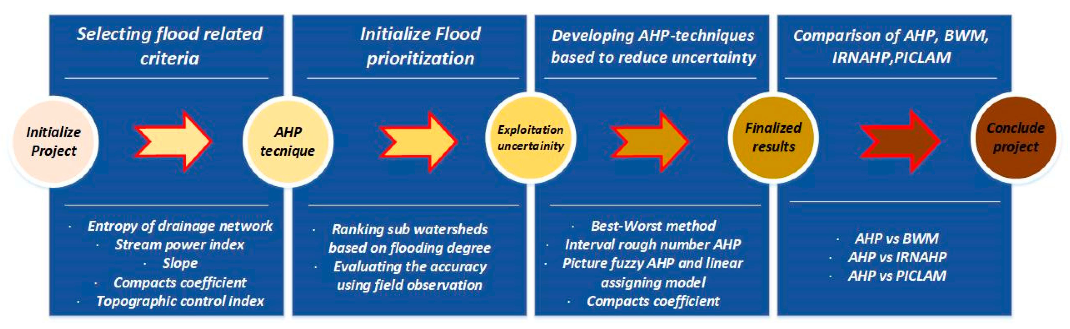
2. Materials and Methods
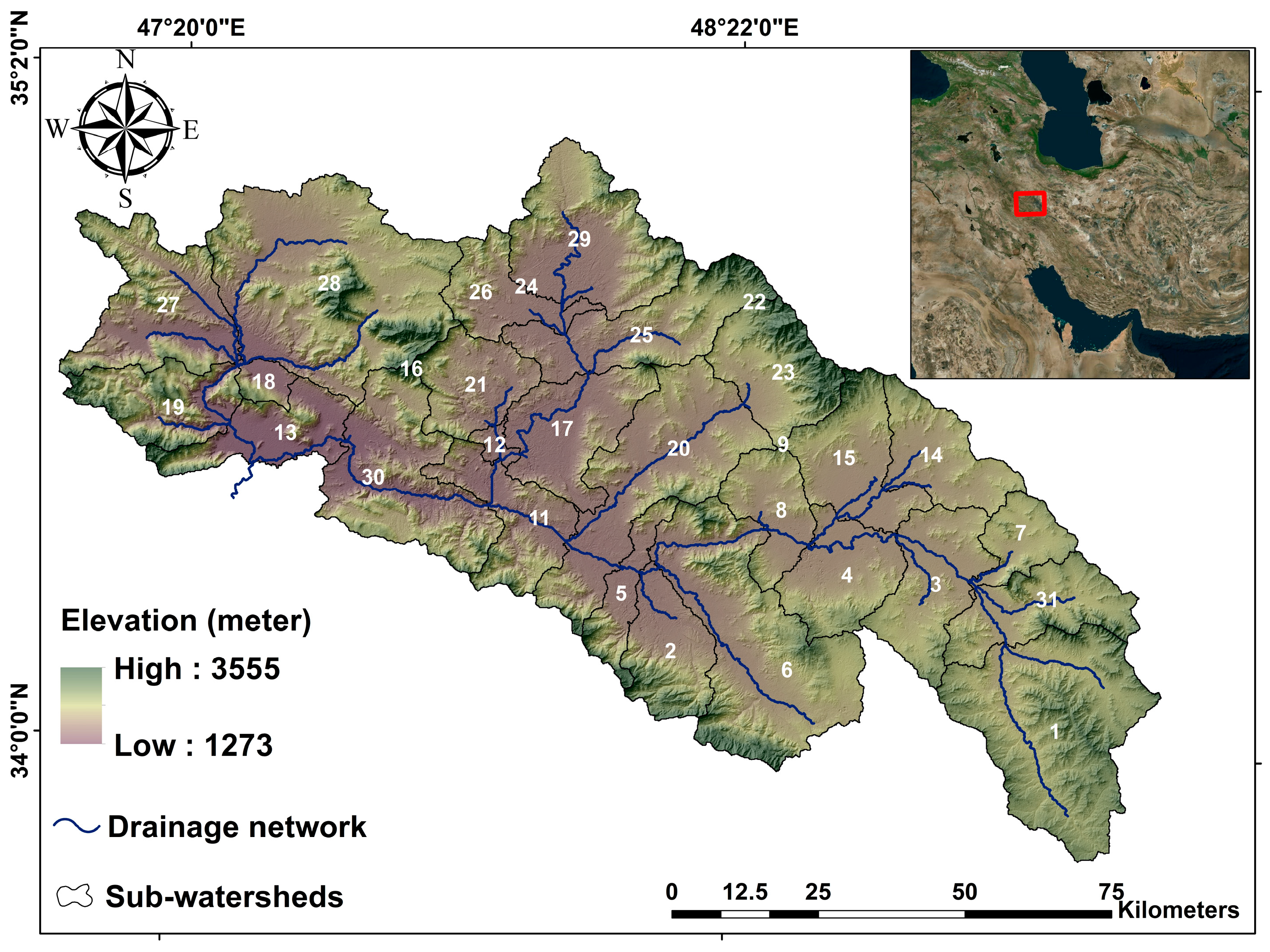
2.1. Study Area

The Sad-Kalan watershed is located west of Iran, including the Hamadan and Lorestan provinces (from 34,000′0″ N to 35,022′0″ N and from 47,020′0″ E to 48,022′0″ E), and covers approximately 10,358.9 km2 (Figure 1) The case study is one of the main headwaters of the Karun River, which is Iran’s most affluent and only navigable river. The watershed contains 25 sub-watersheds. It is situated in a moderate climate in the summer (August) and a cold and snowy climate in the winter (February). The annual average temperature is +9.7 °C, and the annual average rainfall is 313 mm, which occurs mainly between February and April.

2.2. Data and Methodology

The main framework of the current study to assess flood hazards and rank sub-watersheds was adopted using a GIS-based multi-criteria decision analysis (Figure 2). Due to the existence of GIS, scholars can handle large amounts of data and combine the intrinsic or value-based knowledge involved in MCDA. Based on an extensive literature review, our experience, availability of data, field observation, and duplication of factors, seven flood hazard-driven factors, i.e., entropy of the drainage network, slope, topographic control index (TCI), and compactness coefficient (Cc), were investigated to provide a flood hazard ranking map. Subsequently, a short description of the mentioned driving factors was carried out.
Entropy of a drainage network: The drainage network and its features, such as density, length, and bifurcation, are the most important geomorphological features of sub-watersheds that influence soil erosion and flood peak through direct and indirect effects. The direct effects refer to the relationship between flood features (e.g., velocity and depth) and the drainage network, while indirect terms are used to describe the role of the drainage network as a geological index. The entropy of a drainage network is defined as the state of the art of methodology for describing drainage networks and their complexity, so a higher value of entropy tells us that the desired drainage network has more effect on the flooding degree than a drainage network with low entropy. To calculate the entropy of the drainage network, we used the box-counting method (for more descriptions, refer to Sepehri et al. [28]).
Slope: The slope criterion, as a hydrologic-related morphometric factor, can be used to identify areas susceptible to flooding in low-slope gradients. Low-slope areas behave as ponds that retain surface runoff as temporary storage [11,29,30].
Topographic control index (TCI): Topographic elements, such as slope, contributing areas, and the volumes of depression, are also key factors that significantly influence the flow direction, velocity of runoff, and the potential places where pluvial flooding can occur. For a single depression, the quicker it becomes inundated, the more prone it is to flooding. The time required to fill a depression is affected by the topography of its watershed, such as the watershed area, the watershed slope, and the ponding volume of the depression. A watershed includes the upslope contributing area and the depression itself. To evaluate the flooding risk for each depression, an integrated topography control index, namely TCI, was developed [31].
Compactness Coefficient (Cc): Cc refers to the shape of a sub-watershed, which is calculated based on the ratio of the perimeter of the basin to the circumference of a circular area, which equals the basin area. It is one of the most commonly used morphometric features of watersheds in flooding studies. When the values of Cc tend to be close to one, it means the shape of the watershed is closer to a circle, and, therefore, it has the lowest infiltration capacity and the highest sensitivity to flooding [32,33].
Stream power index (SPI): SPI is one of the most commonly used indicators in drainage network analyses, and it can be used to detect and quantify the power of a flow at a given point on a topographic surface [34,35,36,37].

2.3. Theoretical Backgrounds of Proposed Methods

2.3.1. Analytic Hierarchy Process (AHP)

In 1980, Saaty [38] presented a multilevel and hierarchical structural technique that allows one to solve complex and subjective problems. In the technique, the weights of the criteria and sub-criteria are driven by pairwise comparisons. A matrix concerning the nth decision criteria or sub-criteria is created as follows:
A = a 11 a 12 . . . a 21 a 22 . . . . . . . . . . . . a n 1 a n 2 . . . a 1 n a 2 n . . . a n n , a i j = 11 , a j i = 1 a i j
where a i j shows the relative importance of the criteria/sub-criteria to the criteria/sub-criteria j. The level of importance is calculated based on the experts’ knowledge through a 9-point rating scale, which varies between 1/9 (lowest importance) and 9 (highest importance) (Table 1). In the following stage, the elements of the A matrix must be synthesized and normalized to obtain the rank criteria/sub-criteria as A matrix:
A = a 11 a 12 . . . a 21 a 22 . . . . . . . . . . . . a n 1 a n 2 . . . a 1 n a 2 n . . . a n n , a i i = a i j / j = 1 n a i j
Since the weights of the criteria/sub-criteria are calculated based on experts’ knowledge, it is necessary to evaluate the consistency ratio (CR) of matrix A regarding its significant degree of uncertainty. If the CR is < 0.1 , it can be assumed that the mentioned matrix has enough consistency. The rate of consistency can be expressed as follows:
C R = C I / R I
where RI (random index) is a random index that is determined based on randomly generated 500 matrixes [36], and the consistency index (CI) is calculated based on the maximum eigenvector ( λ m a x ) of the A matrix and n (number of criteria/sub-criteria), given as follows:
C I = ( λ m a x n ) / ( n 1 )

2.3.2. IRNAHP

In a pure AHP, each individual decision regarding the weights of criteria and sub-criteria is expressed in rough values. In this state, decision-makers often face a dilemma in allocating relative importance to selected criteria and sub-criteria, and consequently, subjectivity, imprecision, and uncertainty rise in the process of decision-making. In recent years, a new concept in the IRN-based rough numbers theory has been introduced to deal with uncertainty and imprecision. In this regard, the combination of IRN and pure AHP, known as IRAAHP, means that scholars can better deal with the uncertainties of rough numbers. The IRAAHP algorithm is described as follows:
The algorithm of IRNAHP
  • IRN Mathematical Model
Suppose that there is a set of k decision-maker (DM) preferences as R = I 1 , I 2 , , I k , and all its objects are defined in a universe and represent DM preferences. Each object in an R set is defined by the interval I i = I l i , I u i , which is subject to I l i I u i 1 i m . I l i and I u i denote the lower and upper limits of the i class, respectively. If I l i and I u i satisfy I l 1 < I l 2 < , , < I l k and I u 1 < I u 2 < , , < I u k 1 k m , respectively, then R l = ( I l 1 , I l 2 , , I l j ) and R u = ( I u 1 , I u 2 , , I u j ) can be defined. In this state, the lower approximations ( A p r ) of I l i and I u i are represented as follows:
A p r _ I l i = Υ U / R l ( Υ ) I l i
A p r _ I u i = Υ U / R u ( Υ ) I u i
The upper approximations of I l i and I u i are expressed as follows:
A p r ¯ I l i = Υ U / R l ( Υ ) I l i
A p r ¯ I u i = Υ U / R u ( Υ ) I u i
The lower limits of I l i and I u i and, consequently, their upper limits are expressed as follows:
L i m _ I l i = 1 M L R l ( Υ ) Υ A p r _ I l i
L i m _ I u i = 1 M L R u ( Υ ) Υ A p r _ I u i
The upper limits are expressed as follows:
L i m ¯ I l i = 1 M U R l ( Υ ) Υ A p r ¯ I l i
L i m ¯ I u i = 1 M U R u ( Υ ) Υ A p r ¯ I u i
where M L and M U represent the number of objects in the lower/upper approximations of I l i and I u i , respectively.
The rough boundary (RB) for the lower/upper approximations of I l i and I u i can be defined as follows:
Rough boundary I l i :
R B I l i = L i m ¯ I l i L i m _ I l i
Rough boundary I u i :
R B I u i = L i m ¯ I u i L i m _ I u i
Then, the rough boundary concatenation (RC) classes of I l i and I u i are expressed as follows:
R C I l i = L i m ¯ I l i , L i m _ I l i
R C I u i = L i m ¯ I u i , L i m _ I u i
Finally, the interval rough number (IRN) of the I i object can be concluded as follows:
I R N = R C I l i , R C I u i
Interval Rough Numbers AHP (IRNAHP) Mathematical Model
In order to integrate the IRN and pure AHP, the elements of the matrix are transferred to the interval rough number I R N a i j , and the next stages of the pure AHP are repeated. Therefore, three to five stages are needed to obtain the IRNAHP mathematical model, as follows:
Stage 1: Establishing the pairwise comparison matrixes by k experts as follows:
1 a 12 e ; a 12 e a 21 e ; a 21 e 1 a 1 n e ; a 1 n e a 2 n e ; a 2 n e a n 1 e ; a n 1 e a n 2 e ; a n 2 e 1 ; 1 i , j n ; 1 e k
where a i j e and a i j e are the relative importance of the criteria/sub-criteria i to the criteria/sub-criteria j, which are selected based on Saaty’s 9-point rating. If every expert has vagueness for selecting 2 values between the Saaty’s 9-point rating, the a i j e a i j e is established. If there is no vagueness in selecting, the e expert chooses one value, and, in this state, we have the following: a i j e = a i j e .
Stage 2: Calculating the consistency rate for every expert. This stage is similar to the AHP pure one, with the difference that there are two consistency rates, one of which is for upper approximations ( C R e ) and the other one is for lower approximations ( C R e ) . The final CR is calculated based on C R e + C R e / 2 .
Stage 3: Calculating the concatenation of interval rough number matrices in Stage 1 to obtain a * L and a U .
a L = a 11 1 L , a 11 1 L , , a 11 k L a 12 1 L , a 12 1 L , , a 12 k L a 21 1 L , a 21 1 L , , a 21 k L a 22 1 L , a 22 1 L , , a 22 k L a 1 n 1 L , a 1 n 1 L , , a 1 n k L a 2 n 1 L , a 2 n 1 L , , a 2 n k L a n 1 1 L , a n 1 1 L , , a n 1 k L a n 2 1 L , a n 2 1 L , , a n 2 k L a n n 1 L , a n n 1 L , , a n n k L
a U = a 11 1 U , a 11 2 U , , a 11 k U a 12 1 U , a 12 2 U , , a 12 k U a 21 1 U , a 21 2 U , , a 21 k U a 22 1 U , a 22 2 U , , a 22 k U a 13 1 U , a 13 2 U , , a 1 n k U a 23 1 U , a 23 2 U , , a 2 n k U a n 1 1 U , a n 1 2 U , , a n 1 k U a n 2 1 U , a n 2 2 U , , a n 2 k U a n n 1 U , a n n 2 U , , a n n k U
a i j L = a i j 1 L , a i j 1 L , , a i j k L   and   a n 1 U = a i j 1 U , a i j 2 U , , a i j k U
Using Equations (4)–(16), each element of the above matrices is transferred to the rough boundary concatenation (RC), i.e., R C a i j k L = L i m _ a i j k L , L i m ¯ a i j k L and R C a i j k U = L i m _ a i j k L , L i m ¯ a i j k L . Then, using Equations (20) and (21), the rough boundary concatenation (RC) of a L and a U are calculated.
R C a i j L = R C a i j 1 L , a i j 1 L , , a i j e L = a i j L = 1 m e = 1 m a i j e L a i j U = 1 m e = 1 m a i j e U
R C a i j U = R C a i j 1 U , a i j 2 U , , a i j e U = a i j L = 1 m e = 1 m a i j e L a i j U = 1 m e = 1 m a i j e U
Then, using R C a i j L and R C a i j U , the lower and upper limits of I R N a i j , I R N a i j = R C a i j L , R C a i j U , are obtained. The I R N a i j matrix can be shown as follows:
a = 1 I R N ( a 12 ) I R N ( a 21 ) 1 I R N ( a 1 n ) I R N ( a 2 n ) I R N ( a n 1 ) I R N ( a n 2 ) 1
Stage 4: Defining the rank of each criterion (interval rough weighted coefficient), I R N ( w j ) . The vector is calculated based on Equations (24) and (25).
I R N ( w i j ) = w i j L , w i j U , w i j L , w i j U = I R N a i j j = 1 n I R N a i j = a i j L , a i j U , a i j L , a i j U j = 1 n a i j L , j = 1 n a i j U , j = 1 n a i j L , j = 1 n a i j U
W = 1 w 12 L , w 12 U , w 12 L , w 12 U w 21 L , w 21 U , w 21 L , w 21 U 1 w n 1 L , w n 1 U , w n 1 L , w n 1 U w n 2 L , w n 2 U , w n 2 L , w n 2 U w 1 n L , w 1 n U , w 1 n L , w 1 n U w 2 n L , w 2 n U , w 2 n L , w 2 n U 1
Finally, the interval rough weighted coefficient, I R N ( w j ) , can be calculated using Equation (26).
I R N ( w j ) = w i j L , w i j U , w i j L , w i j U j = 1 n w i j L , j = 1 n w i j U , j = 1 n w i j L , j = 1 n w i j U / n
S u b j e c t o : 0 w j L w j L w j U w j U 1 1

2.3.3. Best–Worst Method (BWM)

The best–worst method (BWM), developed by Rezaei [39], is one of the latest MCDA methods for dealing with multi-objective complex systems. Compared to AHP, BWM requires fewer pairwise comparisons to obtain the weights of criteria and sub-criteria, so it only requires pairwise comparisons, whereas in AHP, these comparisons are increased until one of the main sources of rising uncertainty is reduced.
The algorithm of the best–worst method (BWM) can be described as follows:
Stage 1. Selection of a set of desired criteria/sub-criteria, and determination of the best/worst (most/least important) of them.
Stage 2. Determination of preferences of the best criterion over others (BO) and vice versa, i.e., preferences of all criteria over the worst criterion, using a 9-point rating scale (Table 1).
A B = a B 1 , a B 2 , , a B n
A W = a 1 W , a 2 W , , a n W
where a B n indicates the preferences of the best criterion and a n W shows the preferences of the worst criterion.
Stage 3. Finding the optimal weights w 1 , w 2 , , w 3 by solving the following model:
min ξ s . t . w B w j a B j ξ , f o r a l l j w j w W a j W ξ , f o r a l l j j w j = 1 w j = 0 , f o r a l l j
Stage 4. Checking the consistency as follows:
C o n s i s t e n c y   R a t i o = ξ C o n s i s t e n c y   I n d e x
The consistency index is calculated and shown in Table 2. The consistency ratio varies between 0 and 1, where the lower values of the consistency ratio show a more consistent preference matrix.

2.3.4. Picture Fuzzy Analytic Hierarchy Process and Picture Fuzzy Linear Assignment (PICALAM)

Gündodu et al. [27] introduced the picture fuzzy analytic hierarchy process and picture fuzzy linear assignment, a novel technique of hybrid multi-attribute decision-making using AHP and LAM under the picture fuzzy concept to reduce the hesitancy or uncertainty of decision-makers’ judgments due to the lack of information or motivation on the examined problem. On Saty’s 9-point rating system, the picture fuzzy is the most recent expansion of fuzzy logic and can be used as a valuable tool to deal with a decision maker’s imprecision and uncertainty. (See the following for more information on the picture fuzzy analytic hierarchy process and picture fuzzy linear assignment algorithm.)
Definition 1:
The single-valued PFS of ÃU of the universe of discourse U can be defined as follows:
à p = u , μ A ~ p u , I A ~ p u , ν A ~ p u u U
where
μ A ~ p u : U 0,1 , I A ~ p u : U 0,1 , ν A ~ p u : U 0,1
0 < μ A ~ p u + I A ~ p u + ν A ~ p u < 1 u U
where  μ A ~ p u  is the degree of membership;  I A ~ p u  is the degree of non-membership, and  ν A ~ p u  is the indeterminacy of  u  to  Ã p , respectively. Additionally, the degree of refusal of  u  can be defined as follows:  χ Ã p = 1 μ A ~ p u + I A ~ p u + ν A ~ p u .
Definition 2:
The basic operations of PFS can be defined as follows:
à p B ~ p = μ A ~ p + μ B ~ p μ A ~ p μ B ~ p , I A ~ p I B ~ p , ν A ~ p ν B ~ p
  • Addition
  • Multiplication
B ~ p à p = μ A ~ p μ B p , I A ~ p I B ~ p , ν A ~ p + ν B ~ p ν A ~ p ν B ~ p
  • Multiplication by a scalar; λ > 0
λ . Ã p = 1 1 μ A ~ p λ , I A ~ p λ , ν A ~ p λ
Power of  A ~ p , λ > 0
à p λ = μ A ~ p λ , I A ~ p λ , 1 1 ν A ~ p λ
Definition 3:
The PFS-weighted geometric (PFWG) mean given that  w = w 1 , w 2 , , w n ,  w 0,1 ,  j = 1 n w n = 1  can be defined as one of the following equations: 
P F W G w à 1 , , à n = j = 1 n μ A ~ j w j , j = 1 n I A ~ j w j , 1 j = 1 n 1 ν A ~ j w j
 
P F W G w A ~ 1 , , A ~ n = 1 j = 1 n 1 μ A ~ j w j , j = 1 n I A ~ j w j , 1 j = 1 n ν A ~ j w j
Definition 4:
To de-fuzzify, rank, and compare the PFS sets, the following score (SC) and accuracy (AC) functions can be used:
S C 1 A ~ p = 0.5 1 + 2 μ A ~ p ν A ~ p I A ~ p 2
S C 2 A ~ p = 2 μ A ~ p ν A ~ p I A ~ p 2
S C 3 A ~ p = μ A ~ p ν A ~ p
A C A ~ p = μ A ~ p u + I A ~ p u + ν A ~ p u
After calculating the score and accuracy functions, the dominance rules can be written as follows:
i f   S C A ~ p > S C B ~ p ,   t h e n   A ~ p > B ~ p i f   S C A ~ p = S C B ~ p   a n d   A C A ~ p > A C B ~ p ,   t h e n   A ~ p > B ~ p i f   S C A ~ p = S C B ~ p   a n d   A C A ~ p < A C B ~ p ,   t h e n   A ~ p < B ~ p i f   S C A ~ p = S C B ~ p   a n d   A C A ~ p = A C B ~ p ,   t h e n   A ~ p = B ~ p
The stages listed below describe the picture blurry, which is related to LAM. The weights of criteria using picture fuzzy are determined in Stage 1, while the rank of alternatives is calculated in Stage 2.
Stage 1: Picture fuzzy analytic hierarchy process.
1.1. Using pairwise comparison matrices for the weights of the criteria
The criteria are compared in this step by the decision-makers. They chose a value from Saaty’s nine-point scale based on their job, and the value was then translated to the associated picture fuzzy digits (Table 3). Since the values chosen from Table 1 are based on experts’ preferences, it is important to double-check the consistency ratio (CR) of each pairwise comparison, which is calculated using Equation (2), as well as the consistency index (CI) and random index (RI).
1.2. To aggregate the decision-makers’ assessments, we used a weighted geometric (PFWG) mean. There can be different comparison matrixes w ~ j l o c a l in decision-making situations because there are multiple decision-makers. It is necessary to employ geometric means (Equation (38)) to unify all comparison matrices w ~ j g l o b a l in the next steps. Eventually, the final picture fuzzy weight w ~ j f i n a l must be calculated as follows:
w ~ j f i n a l = w ~ j l o c a l w ~ j g l o b a l
1.3. De-fuzzification of w ~ j f i n a l .
It is required to export w ~ j f i n a l as a defuzzified value in this stage in order to use w ~ j f i n a l from the criteria as a weight for ranking the sub-watersheds (Stage 2).
Stage 2: Using the PFS to rank the alternatives.
2.1. This point is similar to Stage 1’s point 1.1. The difference is that decision-makers’ individual judgments are based on alternatives in the form of decision matrices (Table 4).
2.2. The individual decision matrices from the previous point were aggregated using Equation (37), as shown in Table 5.
2.3. Defuzzification of the aggregated matrix using Equation (40) was performed to compare and rank options that are connected to each other.
2.4. Determination of the rank frequency matrix, which includes associated elements that show the number of times alternative m dominates on the nth criterion (Table 6).
2.5. Determination of the weighted rank frequency matrix Π i k , which measures the contribution of the mth alternative to the overall ranking (Equation (45) and Table 7).
Π i k = w i 1 + w i 2 + + w i λ m m
2.6. Construction of the linear assignment model based on Π i k and permutation matrix P (m*m) as follows:
max i = 1 m k = 1 m Π i k . P i k s . t . k = 1 m P i k = 1 , i = 1,2 , , m i = 1 m P i k = 1 , i = 1,2 , , m P i k = 0   o r   1   f o r   a l l   i   a n d   k .
2.7. Using Equation (46) to obtain the optimal permutation matrix ( P ) .
2.8. Obtaining the rank of alternatives as follows:
P A = P A 1 A 2 A m

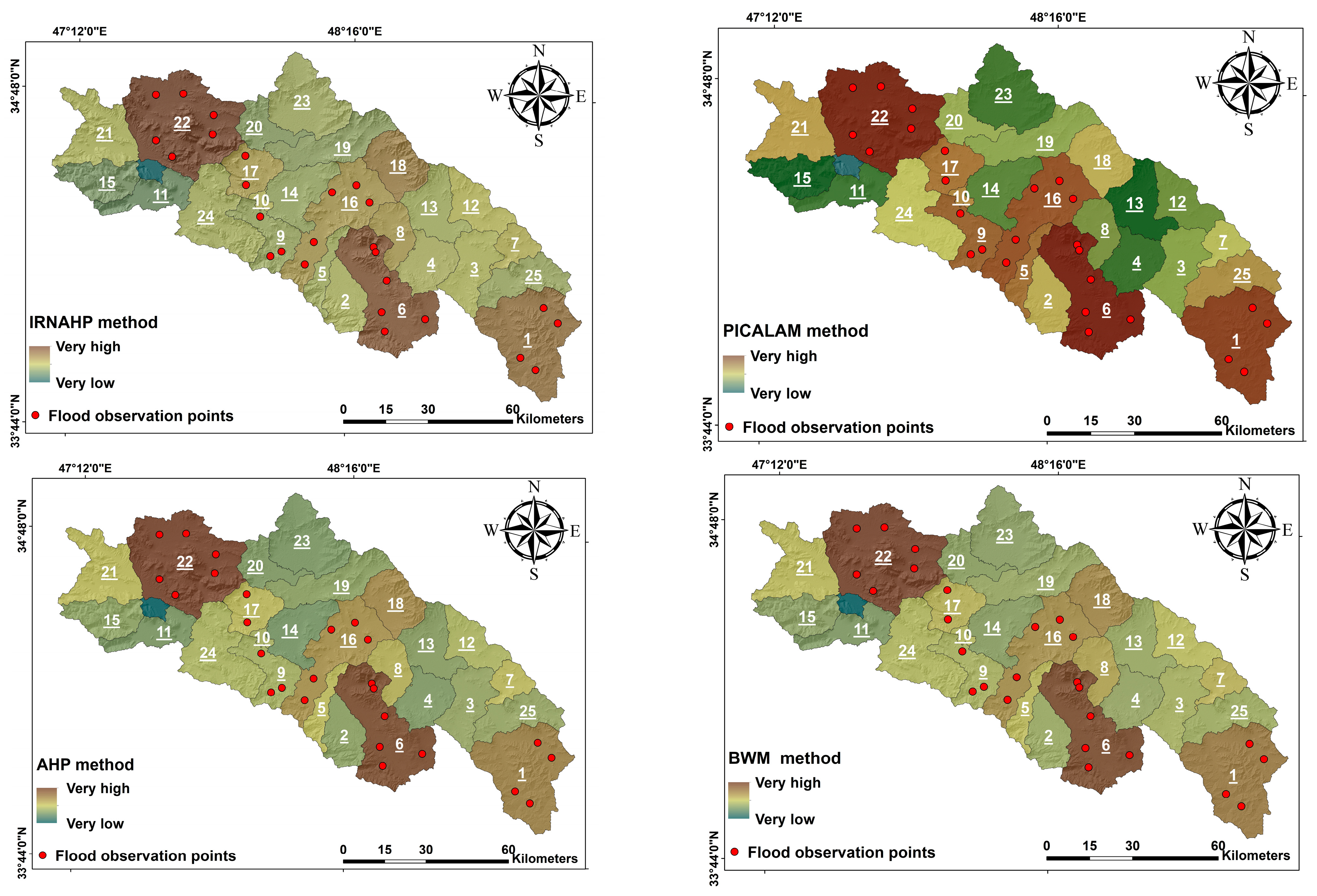
3. Analysis and Results

3.1. Morphometric Parameters

Morphometric parameters of drainage basins have been successfully applied to simulate Earth’s surface processes and landforms, incorporating hydrological, geological, and geo-morphological setups at different scales [23,40,41,42,43]. It can be observed that the entropy of the drainage network ranges between 0.03 (sub-watershed #6) and 0.145 (sub-watershed #13). According to the results of a TCI, the highest value of this criterion is related to sub-watershed #12 (−0.81) and vice versa, and sub-watershed #15 acquired the lowest value (−1.29). The highest and lowest values of the slope criterion are related to sub-watershed #15 (40.65) and sub-watershed #3 (12.22), respectively. The values of SPI indicate that sub-watershed #15 (−1.47) and sub-watershed #4 (−3.73) have been ranked in the first and last positions, respectively. According to the results of the Cc, it can be concluded that sub-watershed #5 (2.78) gained the highest values and sub-watershed #18 (1.58) received the lowest values, respectively (Table 8).

3.2. Ranking of Sub-Watersheds Using the AHP Technique

During the analysis, the weights of the morphometric parameters are calculated based on their importance in the case study of area floods. The weight assignment for each criterion was calculated based on the local characteristics of each criterion, and the opinions of three experts in the field of hydrology science are shown in Table 9. Based on the criteria weights, the most important criterion regarding the occurrence of floods in the study area is related to the entropy of the drainage network. The Cc weight was defined as the least important criterion. The remaining criteria, i.e., SPI, TCI, and slope, are next in order of importance. After the weight assignment to each criterion, the total weight for each sub-watershed was computed using a simple weighted sum, which is as follows:
H i = j w j x i j
where w j is the weight of the criterion jth and x i j is the normalized value of the criterion jth. The weights of each criterion are given in Table 9. Additionally, for each pairwise comparison matrix, the calculated consistency ratio (CR) showed that the mentioned matrices have enough consistency.
In the BWM, based on the judgments of the decision-makers, the entropy of the drainage network was chosen as the best criterion (the most important flood-related criterion), and, at the opposite point, the Cc was selected as the worst criterion (the least important flood-related criterion). Then, using the best/worst criterion, the BO and OW vectors were determined, and, finally, the average weight of the criteria was calculated as follows: entropy of drainage network (0.462), SPI (0.203), TCI (0.133), slope (0.136), and Cc (0.067) (Table 9). Finally, using Equation (1), the ranking of the sub-watersheds was acquired. On the other hand, in the IRNAHP, the entropy of the drainage network and the Cc were known as the most and least important flood-related criteria (Table 9).
Based on Table 10, the local and global weights of each criterion were calculated (Table 10), and the weights of the alternatives (sub-watersheds) are shown in Table 11. Consequently, by using the mentioned weights, the weighted frequency rank matrix was determined (Table 12). Finally, according to the weighted frequency rank matrix, the permutation matrix in Table 13 was acquired to rank the sub-watersheds based on the flood risk degree. Finally, by using Equation (42), the ranking of the sub-watersheds was acquired.

4. Discussion

Based on the results of the AHP technique, the sub-watersheds #22, #1, and #6 have very high flood probabilities, while the sub-watersheds #23, #11, and #14 have very low flood probabilities (Figure 3). Based on Figure 3, it can be observed that the sub-watersheds #22, #1, and #6 receive the lowest value of entropy of the drainage network, and the SPI criteria in these sub-watersheds are nearly high. These results are consistent with the findings of Sepehri et al. [28] and Zhang et al. [44] in that they emphasize the drainage network as the most important geomorphology feature of a watershed that has the main effect on flooding and sediment yield, so that a watershed that has a drainage network with more complex features (such as more entropy/length/stream power) has more susceptibility to flooding and sediment yield than a watershed with a low-complexity drainage network. The flood observation points, which were prepared by the General Department of Natural Resources of Hamadan Province and are shown as red circles in Figure 3, represent that the accuracy of the AHP output regarding flood ranking is acceptable, so that the high number of flood observation points are located in sub-watersheds #22, #1, and #6.
In the BWM method, the results show the same result as with the AHP technique, so that sub-watersheds #22, #1, and #6 are positioned at the first rank of flooding degree, while in contrast, sub-watersheds #23, #14, and #11 have the last rank of flooding degree. However, these same results show that the BWM method is less time-consuming than the AHP technique because, in this study, to reach the weights of the used criteria, the BWM method only needed 21 pairwise comparison matrices (for three experts), whereas in the AHP technique, this number of pairwise comparisons is significantly increased, i.e., 60 pairwise comparisons. It is obvious that in other studies with a higher number of criteria, the difference between the pairwise comparisons will be dramatically increased, and, in this state, the uncertainty of the considerations will be increased [19,25,26]. In the IRNAHP method, the sub-watersheds #22, #1, and #6 with the highest elevation are located in the first three ranks, respectively, and, in contrast, sub-watersheds #20, #15, and #11 are specified in the last rank and are the most susceptible to flooding, respectively. Even though these same results through the IRNAHP can be acquired by solving complex algorithms rather than the AHP technique, it must be noted that in MCDA studies that involve a high number of criteria and are associated with a large amount of uncertainty and subjectivity, the experts face a dilemma in choosing a crisp value as the initial weight for each criterion. Therefore, in these studies, IRN can be used as an effective tool to exploit uncertainty [26,45]. The output of PICALAM shows that the sub-watersheds #6, #22, and #1 are posited in ranks 1, 2, and 3, whereas the sub-watersheds #4, #15, and #13 are located in the last ranks. The first three ranks are similar to the previous methods, but the last three ranks are quite different. According to Figure 3, it can be observed that in sub-watersheds #4, #15, and #13, despite having the highest value of entropy of the drainage network and the lowest value of SPI, other flood-related criteria have the lowest relationship with the flooding degree. Additionally, in the PICALAM, the rank of the middle sub-watersheds is not the same as the three remaining methods. For example, the sub-watersheds #16 and #9 in PICALAM have been ranked as the most susceptible areas to flooding (ranks 4 and 5). The flood observation point in sub-watersheds #16 and #9 proves that these sub-watersheds have been ranked correctly. Therefore, it can be concluded that the PICALAM method has better performance than other methods. In PICALAM, there are two main advantages over other methods that can enhance its performance. (1) In the PICLAM, the values of the nine-point rating scale will be transferred to their corresponding fuzzy numbers so that these numbers are based on human reasoning and reduce uncertainty [27,46]. (2) One of the main characteristics of watersheds is their spatial variability, which means that the role and importance of each criterion subjected to the desired objective (here, flooding degree) will differ from one sub-watershed to the next. On the other hand, each criterion has an interrelationship with other criteria that cannot be considered due to a lack of data or an increase in the number of used criteria. For example, one of the main criteria used in this study is TCI, which represents the capacity of each sub-watershed to retain water and is calculated based on surface features (i.e., slope, upslope contribution area, and water volume). It is obvious that these parameters also depend on soil conductivity and land use, which were not considered in this study. In PICALAM, experts can use global and local weights to assign weights to commonly used criteria. For global weights, on which the AHP, IRNAHP, and BWM methods are based, the weight of each criterion is calculated as general for all sub-watersheds without taking into account the properties of watershed spatial variability. For local weights, the weight of each criterion can be calculated separately without considering other sub-watersheds. Therefore, PICALAM allows for greater flexibility and accuracy in decision-making due to the uncertainty and imprecision of complex decision analyses.

5. Conclusions

In this study, a range of MCDM approaches, such as the AHP, BWM, IRNAHP, and the PICAHP and LAM, were used to rank Sad-Kalan sub-watersheds in terms of flooding degree. To accomplish this, five essential criteria related to flooding, namely entropy of the drainage network, SPI, slope, TCI, and Cc, were chosen. The mentioned MCDM approaches were employed to assign a specific weight to each criterion based on its significance in determining the degree of flooding. Subsequently, by combining the weighted criteria, a flood hazard map was generated. The results indicated that among the MCDM approaches utilized, the PICAHP and LAM method demonstrated superior performance due to its consideration of the spatial variability of watersheds. Additionally, the results revealed that the AHP, BWM, and IRNAHP methods exhibited comparable performance in ranking the sub-watersheds. However, it should be noted that the BWM method stands out for its time-efficient operation in comparison to the other two approaches. Overall, it is important to acknowledge that this study was conducted to assess how human linguistic terms and their quantity influence the uncertainty of flood degree ranking in a case study with only five flood-related criteria. It is worth noting that the performance of the MCDM approaches used may vary significantly in other studies that involve a higher number of criteria and greater complexity. Furthermore, it is essential to recognize that flood hazards, as the initial component of flood risk studies, primarily focus on the physical and climatic aspects of floods. For future studies, it is advisable to incorporate social-economic criteria to facilitate comprehensive flood management.

Author Contributions

V.N.D., N.-M.N., R.B., J.S. and I.E.: formal analysis, investigation, methodology, writing—original draft. M.S., H.N., A.G., V.N.D. and A.T.: resources, writing—review and editing. I.E., C.B.P., S.G.M. and V.N.D.: formal analysis, investigation, supervision, validation, writing—review and editing. All authors have read and agreed to the published version of the manuscript.

Funding

The project is funded by the Deputy for Research and Innovation Ministry of Education, Kingdom of Saudi Arabia for this research through a grant (NU/IFC/2/SERC/-/12) under the Institutional Funding Committee at Najran University, Kingdom of Saudi Arabia.

Institutional Review Board Statement

Not applicable.

Informed Consent Statement

Not applicable.

Data Availability Statement

The data and code in this paper can be obtained by contacting the corresponding author.

Acknowledgments

The authors would like to acknowledge the support of the Deputy for Research and Innovation, Ministry of Education, Kingdom of Saudi Arabia, for this research through a grant (NU/IFC/02/SERC/-/12) under the Institutional Funding Committee at Najran University, Kingdom of Saudi Arabia.

Conflicts of Interest

This manuscript has not been published or presented elsewhere in part or entirety and is not under consideration by another journal. There are no conflicts of interest to declare.

References

  1. Ramkar, P.; Yadav, S.M. Flood risk index in data-scarce river basins using the AHP and GIS approach. Nat. Hazards 2021, 109, 1119–1140. [Google Scholar] [CrossRef]
  2. Papilloud, T.; Röthlisberger, V.; Loreti, S.; Keiler, M. Flood exposure analysis of road infrastructure—Comparison of different methods at national level. Int. J. Disaster Risk Reduct. 2020, 47, 101548. [Google Scholar] [CrossRef]
  3. Guha-Sapir, D.; Vos, F.; Below, R.; Ponserre, S. Annual Disaster Statistical Review 2011: The Numbers and Trends; Institute of Health and Society (IRSS): Brussels, Belgium, 2012. [Google Scholar]
  4. Mohleji, S.; Pielke, R., Jr. Reconciliation of trends in global and regional economic losses from weather events: 1980–2008. Nat. Hazards Rev. 2014, 15, 04014009. [Google Scholar] [CrossRef] [Green Version]
  5. Shabanikiya, H.; Seyedin, H.; Haghani, H.; Ebrahimian, A. Behavior of crossing flood on foot, associated risk factors and estimating a predictive model. Nat. Hazards 2014, 73, 1119–1126. [Google Scholar] [CrossRef]
  6. Yari, A.; Ardalan, A.; Ostadtaghizadeh, A.; Zarezadeh, Y.; Boubakran, M.S.; Bidarpoor, F.; Rahimiforoushani, A. Underlying factors affecting death due to flood in Iran: A qualitative content analysis. Int. J. Disaster Risk Reduct. 2019, 40, 101258. [Google Scholar] [CrossRef]
  7. Sepehri, M.; Malekinezhad, H.; Ilderomi, A.R.; Talebi, A.; Hosseini, S.Z. Studying the effect of rain water harvesting from roof surfaces on runoff and household consumption reduction. Sustain. Cities Soc. 2018, 43, 317–324. [Google Scholar] [CrossRef]
  8. Pham, B.T.; Luu, C.; Van Dao, D.; Van Phong, T.; Nguyen, H.D.; Van Le, H.; von Meding, J.; Prakash, I. Flood risk assessment using deep learning integrated with multi-criteria decision analysis. Knowl. Based Syst. 2021, 219, 106899. [Google Scholar] [CrossRef]
  9. Tang, Z.; Zhang, H.; Yi, S.; Xiao, Y. Assessment of flood susceptible areas using spatially explicit, probabilistic multi-criteria decision analysis. J. Hydrol. 2018, 558, 144–158. [Google Scholar] [CrossRef]
  10. Abdullah, M.F.; Siraj, S.; Hodgett, R.E. An Overview of Multi-Criteria Decision Analysis (MCDA) Application in Managing Water-Related Disaster Events: Analyzing 20 Years of Literature for Flood and Drought Events. Water 2021, 13, 1358. [Google Scholar] [CrossRef]
  11. Fernández, D.; Lutz, M. Urban flood hazard zoning in Tucumán Province, Argentina, using GIS and multicriteria decision analysis. Eng. Geol. 2010, 111, 90–98. [Google Scholar] [CrossRef]
  12. Vojtek, M.; Vojteková, J. Flood susceptibility mapping on a national scale in Slovakia using the analytical hierarchy process. Water 2019, 11, 364. [Google Scholar] [CrossRef] [Green Version]
  13. Sepehri, M.; Malekinezhad, H.; Hosseini, S.Z.; Ildoromi, A.R. Assessment of flood hazard mapping in urban areas using entropy weighting method: A case study in Hamadan city, Iran. Acta Geophys. 2019, 67, 1435–1449. [Google Scholar] [CrossRef]
  14. Schanze, J. Flood Risk Management: Hazards, Vulnerability and Mitigation Measures; Springer: Berlin/Heidelberg, Germany, 2006; pp. 1–20. [Google Scholar]
  15. Tsakiris, G. Flood risk assessment: Concepts, modelling, applications. Nat. Hazards Earth Syst. Sci. 2014, 14, 1361–1369. [Google Scholar] [CrossRef] [Green Version]
  16. Das, S. Geographic information system and AHP-based flood hazard zonation of Vaitarna basin, Maharashtra, India. Arab. J. Geosci. 2018, 11, 576. [Google Scholar] [CrossRef]
  17. El-Magd, S.A.A.; Amer, R.A.; Embaby, A. Multi-criteria decision-making for the analysis of flash floods: A case study of Awlad Toq-Sherq, Southeast Sohag, Egypt. J. Afr. Earth Sci. 2020, 162, 103709. [Google Scholar] [CrossRef]
  18. Khosravi, K.; Shahabi, H.; Pham, B.T.; Adamowski, J.; Shirzadi, A.; Pradhan, B.; Dou, J.; Ly, H.-B.; Gróf, G.; Ho, H.L. A comparative assessment of flood susceptibility modeling using multi-criteria decision-making analysis and machine learning methods. J. Hydrol. 2019, 573, 311–323. [Google Scholar] [CrossRef]
  19. Sepehri, M.; Ildoromi, A.R.; Malekinezhad, H.; Hosseini, S.Z.; Talebi, A.; Goodarzi, S. Flood hazard mapping for the gonbad chi region, Iran. J. Environ. Eng. Sci. 2017, 12, 16–24. [Google Scholar] [CrossRef]
  20. Mahmoud, S.H.; Gan, T.Y. Multi-criteria approach to develop flood susceptibility maps in arid regions of Middle East. J. Clean. Prod. 2018, 196, 216–229. [Google Scholar] [CrossRef]
  21. Malekinezhad, H.; Sepehri, M.; Pham, Q.B.; Hosseini, S.Z.; Meshram, S.G.; Vojtek, M.; Vojteková, J. Application of entropy weighting method for urban flood hazard mapping. Acta Geophys. 2021, 69, 841–854. [Google Scholar] [CrossRef]
  22. Chen, Y.; Yu, J.; Khan, S. The spatial framework for weight sensitivity analysis in AHP-based multi-criteria decision making. Environ. Model. Softw. 2013, 48, 129–140. [Google Scholar] [CrossRef]
  23. Ahmadisharaf, E.; Kalyanapu, A.J.; Chung, E.-S. Spatial probabilistic multi-criteria decision making for assessment of flood management alternatives. J. Hydrol. 2016, 533, 365–378. [Google Scholar] [CrossRef]
  24. Ligmann-Zielinska, A.; Jankowski, P. Spatially-explicit integrated uncertainty and sensitivity analysis of criteria weights in multicriteria land suitability evaluation. Environ. Model. Softw. 2014, 57, 235–247. [Google Scholar] [CrossRef]
  25. Akbari, M.; Meshram, S.G.; Krishna, R.; Pradhan, B.; Shadeed, S.; Khedher, K.M.; Sepheri, M.; Ildoromi, A.R.; Alimerzaei, F.; Darabi, F. Identification of the Groundwater Potential Recharge Zones Using MCDM Models: Full Consistency Method (FUCOM), Best Worst Method (BWM) and Analytic Hierarchy Process (AHP). Water Resour. Manag. 2021, 35, 4727–4745. [Google Scholar] [CrossRef]
  26. Pamučar, D.; Stević, Ž.; Sremac, S. A new model for determining weight coefficients of criteria in mcdm models: Full consistency method (fucom). Symmetry 2018, 10, 393. [Google Scholar] [CrossRef] [Green Version]
  27. Gündoğdu, F.K.; Duleba, S.; Moslem, S.; Aydın, S. Evaluating public transport service quality using picture fuzzy analytic hierarchy process and linear assignment model. Appl. Soft Comput. 2021, 100, 106920. [Google Scholar] [CrossRef]
  28. Sepehri, M.; Ghahramani, A.; Kiani-Harchegani, M.; Ildoromi, A.R.; Talebi, A.; Rodrigo-Comino, J. Assessment of drainage network analysis methods to rank sediment yield hotspots. Hydrol. Sci. J. 2021, 66, 904–918. [Google Scholar] [CrossRef]
  29. Pham, B.T.; Luu, C.; Van Phong, T.; Trinh, P.T.; Shirzadi, A.; Renoud, S.; Asadi, S.; Van Le, H.; von Meding, J.; Clague, J.J. Can deep learning algorithms outperform benchmark machine learning algorithms in flood susceptibility modeling? J. Hydrol. 2021, 592, 125615. [Google Scholar] [CrossRef]
  30. Umer, Y.; Jetten, V.; Ettema, J. Sensitivity of flood dynamics to different soil information sources in urbanized areas. J. Hydrol. 2019, 577, 123945. [Google Scholar] [CrossRef]
  31. Huang, H.; Chen, X.; Wang, X.; Wang, X.; Liu, L. A depression-based index to represent topographic control in urban pluvial flooding. Water 2019, 11, 2115. [Google Scholar] [CrossRef] [Green Version]
  32. Meshram, S.G.; Singh, V.P.; Kahya, E.; Sepehri, M.; Meshram, C.; Hasan, M.A.; Islam, S.; Duc, P.A. Assessing erosion prone areas in a watershed using interval rough-analytical hierarchy process (IR-AHP) and fuzzy logic (FL). Stoch. Environ. Res. Risk Assess. 2021, 36, 297–312. [Google Scholar] [CrossRef]
  33. Olabode, O.F.; Oluwaniyi, O.E.; Adebayo, Q.A.; Asiwaju-Bello, Y.A. Morpho-lithostructural analysis of Ala River basin for flood risk assessment: Geospatial techniques intervention. Earth Sci. Inform. 2020, 13, 773–794. [Google Scholar] [CrossRef]
  34. Mohseni, N.; Salar, Y.S. Terrain indices control the quality of soil total carbon stock within water erosion-prone environments. Ecohydrol. Hydrobiol. 2021, 21, 46–54. [Google Scholar] [CrossRef]
  35. Ahmad, I.; Dar, M.A.; Teka, A.H.; Gebre, T.; Gadissa, E.; Tolosa, A.T. Application of hydrological indices for erosion hazard mapping using Spatial Analyst tool. Environ. Monit. Assess. 2019, 191, 482. [Google Scholar] [CrossRef] [PubMed]
  36. Xu, D.; Zhu, D.; Deng, Y.; Sun, Q.; Ma, J.; Liu, F. Evaluation and empirical study of Happy River on the basis of AHP: A case study of Shaoxing City (Zhejiang, China). Mar. Freshw. Res. 2023. [Google Scholar] [CrossRef]
  37. López-Vicente, M.; Kramer, H.; Keesstra, S. Effectiveness of soil erosion barriers to reduce sediment connectivity at small basin scale in a fire-affected forest. J. Environ. Manag. 2021, 278, 111510. [Google Scholar] [CrossRef] [PubMed]
  38. Saaty, T.L. The Analytic Hierarchy Process; Mc Graw Hill Company: New York, NY, USA, 1980. [Google Scholar]
  39. Rezaei, J. Best-worst multi-criteria decision-making method. Omega 2015, 53, 49–57. [Google Scholar] [CrossRef]
  40. Bhat, M.S.; Alam, A.; Ahmad, S.; Farooq, H.; Ahmad, B. Flood hazard assessment of upper Jhelum basin using morphometric parameters. Environ. Earth Sci. 2019, 78, 54. [Google Scholar] [CrossRef]
  41. Bashir, B. Morphometric Parameters and Geospatial Analysis for Flash Flood Susceptibility Assessment: A Case Study of Jeddah City along the Red Sea Coast, Saudi Arabia. Water 2023, 15, 870. [Google Scholar] [CrossRef]
  42. Keesstra, S.; Nunes, J.P.; Saco, P.; Parsons, T.; Poeppl, R.; Masselink, R.; Cerdà, A. The way forward: Can connectivity be useful to design better measuring and modelling schemes for water and sediment dynamics? Sci. Total Environ. 2018, 644, 1557–1572. [Google Scholar] [CrossRef]
  43. Rodrigo Comino, J.; Keesstra, S.D.; Cerdà, A. Connectivity assessment in Mediterranean vineyards using improved stock unearthing method, LiDAR and soil erosion field surveys. Earth Surf. Process. Landf. 2018, 43, 2193–2206. [Google Scholar] [CrossRef]
  44. Zhang, S.; Guo, Y.; Wang, Z. Correlation between flood frequency and geomorphologic complexity of rivers network–a case study of Hangzhou China. J. Hydrol. 2015, 527, 113–118. [Google Scholar] [CrossRef] [Green Version]
  45. Gigović, L.; Pamučar, D.; Bajić, Z.; Drobnjak, S. Application of GIS-interval rough AHP methodology for flood hazard mapping in urban areas. Water 2017, 9, 360. [Google Scholar] [CrossRef] [Green Version]
  46. Cuong, B.C.; Kreinovich, V. Picture fuzzy sets-a new concept for computational intelligence problems. In Proceedings of the 2013 Third World Congress on Information and Communication Technologies (WICT 2013), Hanoi, Vietnam, 15–18 December 2013. [Google Scholar]
Figure 1. Geographical content of the case study.
Water 15 02128 g001
Figure 2. Flowchart of the used methodology.
Water 15 02128 g002
Figure 3. Flood ranking using AHP, BWM, IRNAHP, and PICAHP and LAM.
Water 15 02128 g003
Table 1. Comparison scale between two criteria [36].
Preference FactorDegree of PreferenceExplanation
1EquallyTwo factors contribute equally to the objective
3ModeratelyExperience and judgment slightly to moderately favor one factor over another
5StronglyExperience and judgment strongly or essentially favor one factor over another
7Very stronglyA factor is strongly favored over another and its dominance is showed in practice
9ExtremelyThe evidence of favoring one factor over another is of the highest degree possible of an affirmation
2, 4, 6, 8IntermediateUsed to represent compromises between the preferences in weights1, 3, 5, 7 and 9
ReciprocalsOppositesUsed for inverse comparison
Table 2. CI values for BWM method.
a B W 123456789
C I m a x ξ 00.441.001.632.303.003.734.475.23
Table 3. Related Saaty’s scale and picture fuzzy numbers (PFNs) for linguistic terms.
Linguistic TermsSaaty’s ScalePicture Fuzzy Numbers (PFNs)
Very High Importance7(0.9, 0.0, 0.05)
High Importance5(0.75, 0.05, 0.1)
Slightly More Importance3(0.6, 0.0, 0.3)
Equally Importance1(0.5, 0.1, 0.4)
Slightly Low Importance1/3(0.3, 0.0, 0.6)
Low Importance1/5(0.25, 0.05, 0.6)
Very Low Importance1/7(0.1, 0.0, 0.85)
Table 4. Individual judgments of decision-makers.
Criteria
AlternativeC1C2Cn
A1 P F 11 k P F 12 k P F 1 n k
A2 P F 21 k P F 22 k P F 2 n k
Am P F m 1 k P F m 2 k P F m n k
Note: Superscript k refers to k decision-maker.
Table 5. Aggregated judgments of decision-makers.
Criteria
AlternativeC1C2Cn
A1 P F W G 11 P F W G 12 P F W G 1 n
A2 P F W G 21 P F W G 22 P F W G 2 n
Am P F W G m 1 P F W G m 2 P F W G n m
Table 6. Rank frequency matrix λ.
Rank
Alternative1st2stmth
A1 λ 11 λ 12 λ 1 n
A2 λ 21 λ 22 λ 2 n
Am λ m 1 λ m 2 λ n m
Table 7. Weighted rank frequency matrix Π .
Rank
Alternative1st2stmth
A1 Π 11 Π 12 Π 1 n
A2 Π 21 Π 22 Π 2 n
Am Π m 1 Π m 2 Π n m
Table 8. Morphometric parameters of sub-watersheds.
Flood-Related Criteria Flood-Related Criteria
Sub-WatershedSlopeTCIEntropyCcSPISub-WatershedSlopeTCIEntropyCcSPI
119.72−1.050.081.82−2.731415.69−1.100.142.11−3.47
221.31−1.180.131.80−2.971540.65−1.290.141.88−1.47
312.22−0.890.142.11−3.641617.24−0.980.082.50−3.12
412.53−0.970.141.93−3.731724.01−1.180.111.72−2.66
523.98−1.200.092.78−2.801825.45−1.080.091.58−2.22
621.26−1.060.032.19−2.781921.30−1.100.142.30−2.76
715.63−0.820.132.13−3.042020.52−1.180.132.42−3.16
814.28−0.860.121.93−3.262128.34−1.140.122.24−2.10
926.78−1.260.122.31−2.492224.50−1.120.031.75−2.62
1016.21−1.140.112.34−3.452320.14−1.160.141.84−3.03
1126.36−1.110.142.41−2.812428.25−1.220.122.11−2.38
1213.05−0.810.142.00−3.292520.66−1.020.142.14−2.80
1313.54−0.900.142.07−3.59
Table 9. Weights of used criteria in AHP, BWM, and IRNAHP.
AHP MethodBWM MethodIRN AHP Method
CriteriaWi
(Expert #1)
Wi
(Expert #2)
Wi
(Expert #3)
Wi
(Expert #1)
Wi
(Expert #2)
Wi
(Expert #3)
w i j L , w i j U , w i j L , w i j U
Entropy0.4880.5930.3910.487 (Best)0.475 (Best)0.423 (Best)[0.46, 0.48], [0.5, 0.52]
SPI0.2280.2440.2150.1890.1880.231[0.21, 0.22], [0.22, 0.23]
TCI0.1420.1500.1630.1420.1410.115[0.15, 0.15], [0.15, 0.16]
Slope0.0870.0840.0990.1140.1410.154[0.06, 0.07], [0.09, 0.09]
Cc0.0560.0440.0530.068 (worst)0.055 (worst)0.077 (worst)[0.03, 0.03], [0.05, 0.05]
Consistently0.020.070.050.0810.0880.038(expert #1)  0.06
(expert #2)  0.079
(expert #3)  0.1
Table 10. Picture fuzzy weights of flood-related criteria.
CriteriaLocal WeightGlobal WeightFinal WeightDeffuzification (Score)
Expert #1En(0.76, 0.24, 0.14)(0.85, 0.4, 0.08)(0.73, 0.05, 0.12)1.31
Expert #2(0.86, 0.14, 0.005)
Expert #3(0.7, 0.3, 0.2)
Expert #1SPI(0.7, 0.3, 0.2)(0.81, 0.48, 0.12)(0.64, 0.09, 0.21)1.03
Expert #2(0.76, 0.24, 0.14)
Expert #3(0.65, 0.35, 0.24)
Expert #1TCI(0.65, 0.34, 0.24)(0.77, 0.53, 0.16)(0.5, 0.18, 0.36)0.55
Expert #2(0.7, 0.3, 0.2)
Expert #3(0.6, 0.4, 0.3)
Expert #1Slope(0.6, 0.4, 0.3)(0.74, 0.56, 0.19)(0.51, 0.16, 0.35)0.59
Expert #2(0.65, 0.34, 0.24)
Expert #3(0.55, 0.45, 0.35)
Expert #1Cc(0.5, 0.4, 0.6)(0.67, 0.58, 0.25)(0.4, 0.23, 0.47)0.21
Expert #2(0.55, 0.4, 0.35)
Expert #3(0.5, 0.4, 0.6)
Table 11. Weights of alternatives (sub-watersheds).
Sub-WatershedEntropySPITCISlopeCc
0(0.95, 0.52, 0.02)(0.94, 0.64, 0.03)(0.9, 0.69, 0.07)(0.91, 0.48, 0.04)(0.84, 0.56, 0.1)
1(0.99, 0.89, 0.002)(0.95, 0.71, 0.02)(0.95, 0.84, 0.029)(0.86, 0.6, 0.08)(0.78, 0.64, 0.15)
2(0.99, 0.94, 0.001)(0.99, 0.95, 0.002)(0.83, 0.54, 0.1)(0.8, 0.47, 0.12)(0.84, 0.73, 0.11)
3(0.99, 0.99, 0.00)(1, 1, 0.00)(0.83, 0.64, 0.11)(0.82, 0.47, 0.12)(0.80, 0.67, 0.14)
4(0.95, 0.6, 0.01)(0.94, 0.66, 0.02)(0.96, 0.86, 0.002)(0.88, 0.65, 0.07)(0.99, 0.99, 0.00)
.
.
.
26(0.97, 0.75, 0.007)(0.90, 0.48, 0.04)(0.95, 0.72, 0.2)(0.92, 0.69, 0.04)(0.89, 0.75, 0.07)
27(0.9, 0.3, 0.03)(0.93, 0.61, 0.029)(0.92, 0.76, 0.04)(0.92, 0.56, 0.03)(0.83, 0.53, 0.1)
28(0.99, 0.99, 0.00)(0.95, 0.73, 0.019)(0.93, 0.84, 0.04)(0.85, 0.58, 0.09)(0.82, 0.6, 0.12)
29(0.97, 0.77, 0.00)(0.92, 0.55, 0.03)(0.95, 0.90, 0.02)(0.91, 0.7, 0.05)(0.85, 0.71, 0.09)
30(0.97, 0.77, 0.00)(0.92, 0.55, 0.03)(0.96, 0.89, 0.02)(0.91, 0.7, 0.05)(0.84, 0.73, 0.1)
Table 12. Weighted frequency rank matrix.
Sub-Watersheds1th2th3th4th5th6th7th 17th18th19th20th21th22th23th24th25th
00.000.592.340.000.000.000.000.000.000.000.000.000.000.000.000.00
10.000.000.000.000.000.000.000.000.000.000.000.000.000.220.000.00
20.000.000.000.000.000.000.001.530.000.550.000.000.000.001.030.59
30.000.000.000.000.000.000.000.000.590.000.000.770.001.310.001.03
40.220.000.000.000.001.311.030.000.000.000.000.000.000.000.000.00
51.310.000.000.810.001.030.000.000.550.000.000.000.000.000.000.00
250.000.000.770.000.000.000.001.030.000.000.000.000.000.000.000.00
260.550.000.000.000.000.590.220.000.000.000.000.000.000.000.000.00
271.631.310.000.000.000.000.000.000.000.000.000.000.000.000.000.00
280.000.000.000.000.000.000.000.590.000.000.000.001.310.000.000.00
290.000.000.000.000.000.000.000.000.000.000.000.000.000.000.000.00
300.000.000.000.000.000.000.000.000.000.000.000.000.000.000.000.00
Table 13. Permutation matrix.
Sub-Watersheds1th2th3th4th5th6th7th 17th18th19th20th21th22th23th24th25th
00010000000000000
10000000000000000
20000000100000000
30000000000000100
40000010000000000
51000000000000000
250000000000000000
260000000000000000
270100000000000000
280000000000001000
290000000000000000
300000000000000000
Disclaimer/Publisher’s Note: The statements, opinions and data contained in all publications are solely those of the individual author(s) and contributor(s) and not of MDPI and/or the editor(s). MDPI and/or the editor(s) disclaim responsibility for any injury to people or property resulting from any ideas, methods, instructions or products referred to in the content.

