Article

Performance Evaluation of Five Machine Learning Algorithms for Estimating Reference Evapotranspiration in an Arid Climate

1
School of Agricultural Engineering, Jiangsu University, Zhenjiang 212013, China
2
Abdullah Alrushaid Chair for Earth Science Remote Sensing Research, Geology and Geophysics Department, College of Science, King Saud University, Riyadh 11451, Saudi Arabia
3
Department of Political Science, Bahauddin Zakariya University, Multan 60000, Pakistan
4
School of Energy & Environment, Power Engineering & Engineering Thermophysics, Southeast University, Nanjing 210096, China
5
Department of Civil Engineering, Faculty of Engineering and Architecture, Erzincan Binali Yıldırım University, 24002 Erzincan, Türkiye
6
School of Transportation, Southeast University, Nanjing 210096, China
7
Agricultural Engineering Department, Faculty of Agriculture, Mansoura University, Mansoura 35516, Egypt
*
Authors to whom correspondence should be addressed.
These authors contributed equally to this work.
Water 2023, 15(21), 3822; https://doi.org/10.3390/w15213822
Submission received: 28 September 2023 / Revised: 28 October 2023 / Accepted: 30 October 2023 / Published: 1 November 2023

Abstract

:
The Food and Agriculture Organization recommends that the Penman–Monteith Method contains Equation 56 (PMF) as a widely accepted standard for reference evapotranspiration (ETo) calculation. Despite this, the PMF cannot be employed when meteorological variables are constrained; therefore, alternative models for ETo estimation requiring fewer variables must be chosen, which means that they perform at least as well as, if not better than, the PMF in terms of accuracy and efficiency. This study evaluated five machine learning (ML) algorithms to estimate ETo and compared their results with the standardized PMF. For this purpose, ML models were trained using monthly time series climatic data. The created ML models underwent testing to determine ETo under varying meteorological input combinations. The results of ML models were compared to assess their accuracy and validate their performance using several statistical indicators, errors (root-mean-square (RMSE), mean absolute error (MAE)), model efficiency (NSE), and determination coefficient (R2). The process of evaluating ML models involved the utilization of radar charts, Smith graphs, heatmaps, and bullet charts. Based on our findings, satisfactory results have been obtained using RBFFNN based on M12 input combinations (mean temperature (Tmean), mean relative humidity (RHmean), sunshine hours (Sh)) for ETo estimation. The RBFFNN model exhibited the most precise estimation as RMSE obtained values of 0.30 and 0.22 during the training and testing phases, respectively. In addition, during training and testing, the MAE values for this model were recorded as 0.15 and 0.17, respectively. The highest R2 and NSE values were noted as 0.98 and 0.99 for the RBFNN during performance analysis, respectively. The scatter plots and spatial variations of the RBFNN and PMF in the studied region indicated that the RBFNN had the highest efficacy (R2, NSE) and lowest errors (RMSE, MAE) as compared with the other four ML models. Overall, our study highlights the potential of ML models for ETo estimation in the arid region (Jacobabad), providing vital insights for improving water resource management, helping climate change research, and optimizing irrigation scheduling for optimal agricultural water usage in the region.

Graphical Abstract

1. Introduction

Providing water to dry and semi-arid regions has become a worldwide challenge. As the global population rises, countries seek new and improved water supply management methods [1]. Improving water management systems and quantitatively scheduling irrigation is crucial to addressing water scarcity issues. Irrigation scheduling, which may be calculated based on evapotranspiration (ET), refers to providing crops with the ideal quantity and timing of water. ET comprises water evaporation into the atmosphere from the soil surface, groundwater table’s capillary fringe, and land-based water bodies. Water flow from the ground to the atmosphere through plants is also included in ET [2]. ET can be directly estimated using lysimeter, eddy covariance system, surface renewal, flux variation and Bowen ratio methods. The high initial, continuing, and maintenance costs of these methods hinder ET estimation [3,4,5]. Therefore, indirect methods are used to quantify ET. The indirect methods use empirical models, categorized into temperature-based, radiation-based, and mass-transfer-based.
Including an estimate of the reference evapotranspiration (ETo) is a basic factor in the empirical models. The difficulty in ascertaining the ET for each individual crop is the underlying factor contributing to this issue. Hence, indirect methods are used to estimate ETo and crop coefficients, which are further utilized to quantify ET for individual crops of interest. The Penman–Monteith (PMF) approach, first introduced by Allen in 1998 and subsequently validated in several climatic conditions [4,6], is now endorsed by the Food and Agriculture Organisation (FAO) of the United Nations and the American Society of Civil Engineers (ASCE) committee. In order to complete PMF ETo calculations, it is important to possess a comprehensive meteorological data collection for several places around the globe. Although the relative importance, interdependence, and interrelationships among the components were previously unclear, recent studies provided ML-based projections of the PMF ETo using a substantial amount of meteorological data [7,8]. Ravindran et al. [9] employed the PMF using the available meteorological data to calculate ETo and then compared it with a deep neural network (DNN) model that only takes sun radiation (Rn) as an input parameter [9]. Zhou et al. [10] investigated the efficacy of machine learning (ML) models, namely deep factorization machine (DeepFM), gradient boosting with categorical feature support (CatBoost), light gradient boosting (LightGBM), extreme gradient boosting (XGBoost), and gradient boosting decision tree (GBDT), for estimating the ETo. Basagaoglu et al. [7] determined that Rn is the most important meteorological variable for determining ETo in a semi-arid location. However, sunshine hours (Sh) might be substituted when Rn is unavailable. The analyses of previous studies revealed that Sh exhibits a closer association with Rn than the other meteorological variables and can be used in the absence of Rn [11,12,13]. The current study used the Sh variable in the analysis for ETo estimation because of the deficiency in the Rn factor.
A major barrier in ETo estimation using the PMF is the unavailability of several meteorological variables and uncertainty in collected data [14,15]. Despite the availability of critical climatic variables, a scarcity of automated weather stations installed at specific sites necessitates the presence of climatic data in numerous locations. Additionally, the use of obsolete weather stations raises issues with data quality. Data calibration is required since the sensor’s inconsistent performance exposes several variances. In this scenario, the inconsistency of ETo estimates opens the door for developing alternative techniques that use fewer inputs to calculate ETo similarly or at least approach the PMF.
Several studies have been conducted that demonstrate an analogy between proposed models based on meteorological data and the PMF. These studies aim to provide alternate ways for ETo estimates because of the frequent absence of meteorological variables [16,17,18,19]. Despite this, ML based on various algorithms (cuckoo, water wave optimization, coactive neuro-fuzzy inference system, decision support system) has become popular for ETo modeling in comparison with empirical equations (the PMF, Hargreaves, Turc, Jensen–Haise, Hargreaves–Samani) using limited climatic data [20,21,22,23,24,25,26,27,28]. The ML models provided good output (ETo) that approached the corresponding empirical equation (PMF) because the optimal selection of input variables against the output factor by adding or eliminating an input variable is considered the main advantage in increasing the efficacy of input versus output relation [29,30,31,32,33,34,35].
The subject of ETo modeling using ML has gained significant attention in recent academic studies, raising interest among hydrologists and meteorologists across different countries. Yin et al. [36] calculated daily ETo in a Hilly interior watershed in northwest China and found support vector machines (SVMs) worked best using daily meteorological data. Wen et al. [37] compared ML with four empirical models in an arid region of China and found temperatures (minimum and maximum) as effective parameters for ETo estimation. Wang et al. [38] analyzed the efficacy of two ML models, namely gene expression programming (GEP) and artificial neural networks (ANNs), in the Karst area of Guangxi Province located in China, for calculating daily ETo. The research showed that ML outperformed with fewer meteorological inputs. Sanikhani et al.’s [39] study showed that the monthly ETo in the Isparta and Antalya region (Turkey) was successfully quantified by employing ML models using limited (temperature) data. In an arid region (Sistan and Baluchestan Province) of Iran, Pour et al. [40] used ML with varying input climatic combinations and found that the ML model (SVM) exhibited superior performance in comparison with the other models for the estimation of ETo. In Jiangxi Province (China), Wu et al. [41] examined the efficacy of ML models using cross-station and synthetic data to measure monthly mean daily ETo and concluded that tree-based ML outperformed other models. Daily ETo using limited climatic data was estimated by Saggi and Jain [42] in Punjab province, India. They found deep learning exhibited superior performance compared with the other models. Similarly, Shiri et al. [43] found good performance of ML for ETo estimation using 29 weather stations in Iran. Tikhamarine et al. [44] compared five ANN-based meta-heuristic algorithms (gray wolf optimizer, multiverse optimizer, particle swarm optimizer, whale optimization algorithm, ant lion optimizer) to estimate monthly ETo using limited data in the Uttarakhand State (Himalayan Region) of India and found that gray wolf optimizer performed well in comparison with the targeted empirical (valiantzas) model. Likewise, Ferreira et al. [45] found that the performance of ML (ANN, GEP) models was good and close to the PMF with minimal climate data in several regions of Brazil. Granata [46] estimated ETo using climate data collected from eddy covariance (EC) flux tower stations set up at a location (Floral City) in central Florida with a humid subtropical environment and found that the chosen ML models were capable of ETo modeling with limited input data in the studied area. Keshtegar et al. [47] compared tree-based and ANN-based ML models with polynomial chaos expansion and the response surface method in the Mediterranean region (Isparta and Antalya) of Turkey for estimating ETo. Likewise, Nourani et al. [48] estimated ETo using climatic data in different climatic regions across five countries (Turkey, NC, Iraq, Iran and Libya) by employing ML ensemble based models and found ANN based ML performed good in comparison to other models. Shiri [49] used limited climatic input in ML models for estimating ETo in an arid region of Iran, and comparison results with six empirical equations showed the supremacy of the chosen ML model.
Recent advances have made it easier to access weather records, yet a lack of meteorological data persists in many locations. Raza et al. [50] systematically reviewed research articles on ETo estimation using ML under Preferred Reporting Items for Systematic Reviews and Meta-Analyses (PRISMA) guidelines and suggested the comparison of ML algorithms for ETo using fewer inputs, especially in developing countries (Pakistan) due to the lack of climatic data. When conventional methods (like the PMF) cannot be used because of excessive input demands or the unavailability of climatic parameters like Rn [36,37,38,39,40,41,42,43,44,45,46,47,48,49], the task of improving methods that rely on fewer climatic inputs and developing ML models for ETo estimation with minimal climatic records becomes of great relevance. Kushwaha et al. [51] concluded that ML might capture time series data without discretization when handled correctly and be able to estimate ETo accurately. Similar findings were obtained by Wu et al. [52] in the Poyang Lake basin in southern China, Roy et al. [53] in the Gazipur District in Bangladesh, Ahmadi et al. [54] in the arid and semi-arid climate of Iran, Sattari et al. [55] in the Corum province of Turkey, and Malik et al. [56] in the Uttarakhand State of India in comparison with the empirical (PMF) method for ETo modeling.
Meteorologists have always monitored the conditions of the atmosphere that impact the weather, but over time the equipment they use has changed. As technology advanced, our scientists began to use more efficient equipment to collect and use weather data. These technological advances enabled meteorologists to make better predictions faster than ever before. These instruments include Doppler radar, Satellite data, Radiosondes, Automated surface-observing systems, and AWIPS (NOAA’s Advanced Weather Information Processing System). The current study obtained climatic data of Jacobabad Meteorological Observatory (JMO) from the Regional Meteorological Center (RMC) Karachi. It is the official meteorological department which is run by the Pakistani government. The current study obtained climatic data (1987–2016) of Jacobabad Meteorological Observatory (JMO) from the Regional Meteorological Center (RMC) Karachi, Pakistan.
According to Germanwatch, the environmental NGO, Pakistan is the eighth most vulnerable country to extreme weather due to climate change. Natural catastrophes, including floods, droughts, and cyclones, have been catastrophic in recent years, resulting in hundreds of deaths, millions of displaced people, and extensive property damage. Jacobabad is an arid city in the province of Sindh, Pakistan. The city’s administration is split into eight different Union Councils. The average summer temperature is 37 °C, while the winters are mild, with an average temperature of 7.7 °C. Precipitation in the city ranged from a high of 838.7 mm in 2022 to a low of 3.3 mm in 1922, with an annual average of 122.5 mm between 1991 and 2020. During the South Asian heat wave in 2022, the average monthly temperature recorded was 43 °C (109 °F), including four days of temperatures equal to or above 50 °C. People in Jacobabad moved during the city’s hottest months (June–August) to avoid the oppressive heat. City heat-reduction services need personal care from government sectors. Being higher in elevation, Quetta (the northern side of Pakistan) is more appealing to locals during the warmer summer. Access to clean water in Pakistan is unreliable and costly because of widespread shortages and significant infrastructure problems. Consequently, monitoring and managing agricultural water usage in this arid region is crucial.
With the recent development in ETo modeling based on ML algorithms using less climatic data, the current study explores five ML algorithms’ performances for estimating ETo in the arid region (Jacobabad) of Sindh province, Pakistan. The main goal of this study is to determine effective climatic variables for ETo estimation. In the current study, a total of 17 different input models were initially formulated based on different combinations made by using the meteorological inputs which are mainly used in the PMF for ETo estimation. We tried to accurately estimate ETo with limited climatic data and the best input combination to calculate ETo, which can be used as an alternative to the PMF in Jacobabad. The novelty of this study is that a comparison of five ML algorithms, namely Iterative dichotomizer (ID3), gradient boosting (GB), Random forest (RF), multilayer neural network (MLNN), and radial basis function neural network (RBFNN), for ETo estimation using less climatic data is not yet explored in an arid region (Jacobabad) of Pakistan. In a nutshell, the following are three objectives of this study:
  • ETo estimation using five ML (ID3, GB, RF, MLNN, and RBFNN) algorithms.
  • Identifying an effective combination of meteorological inputs for ETo estimation.
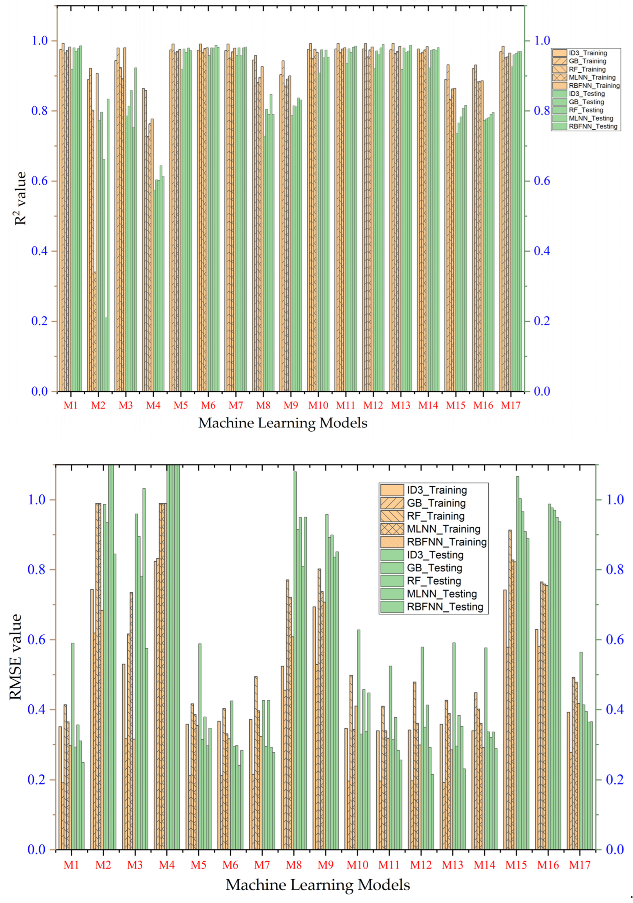
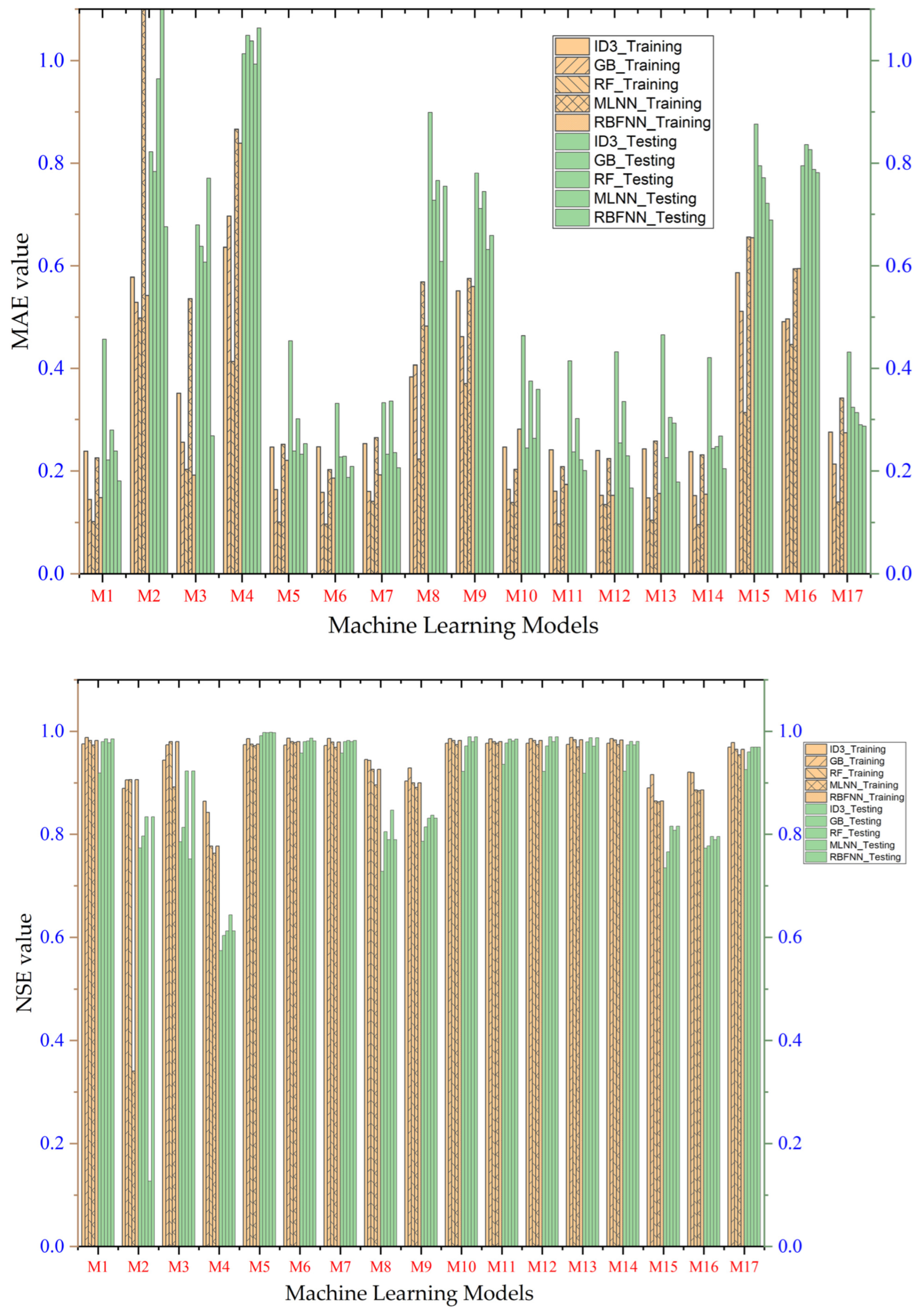
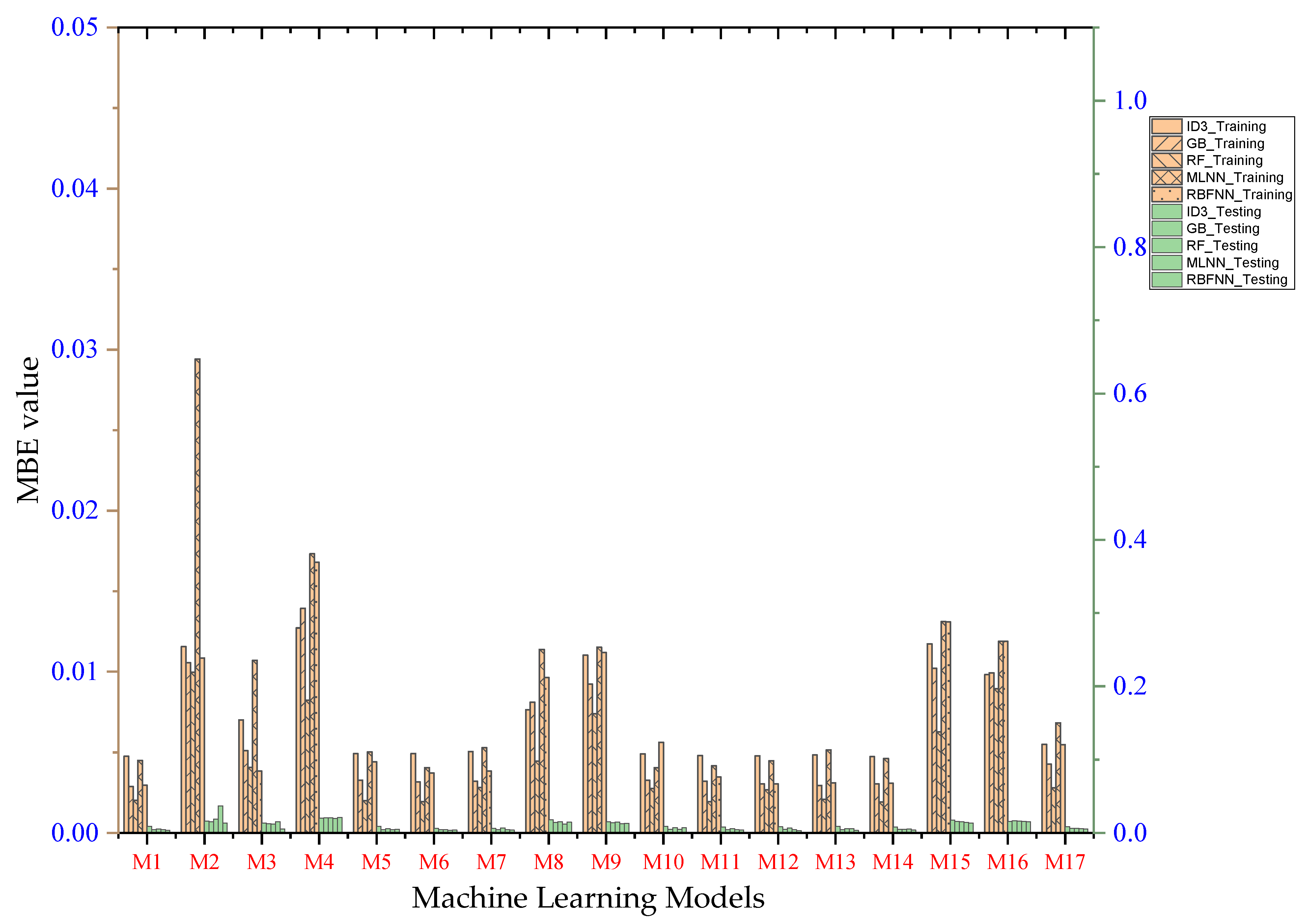
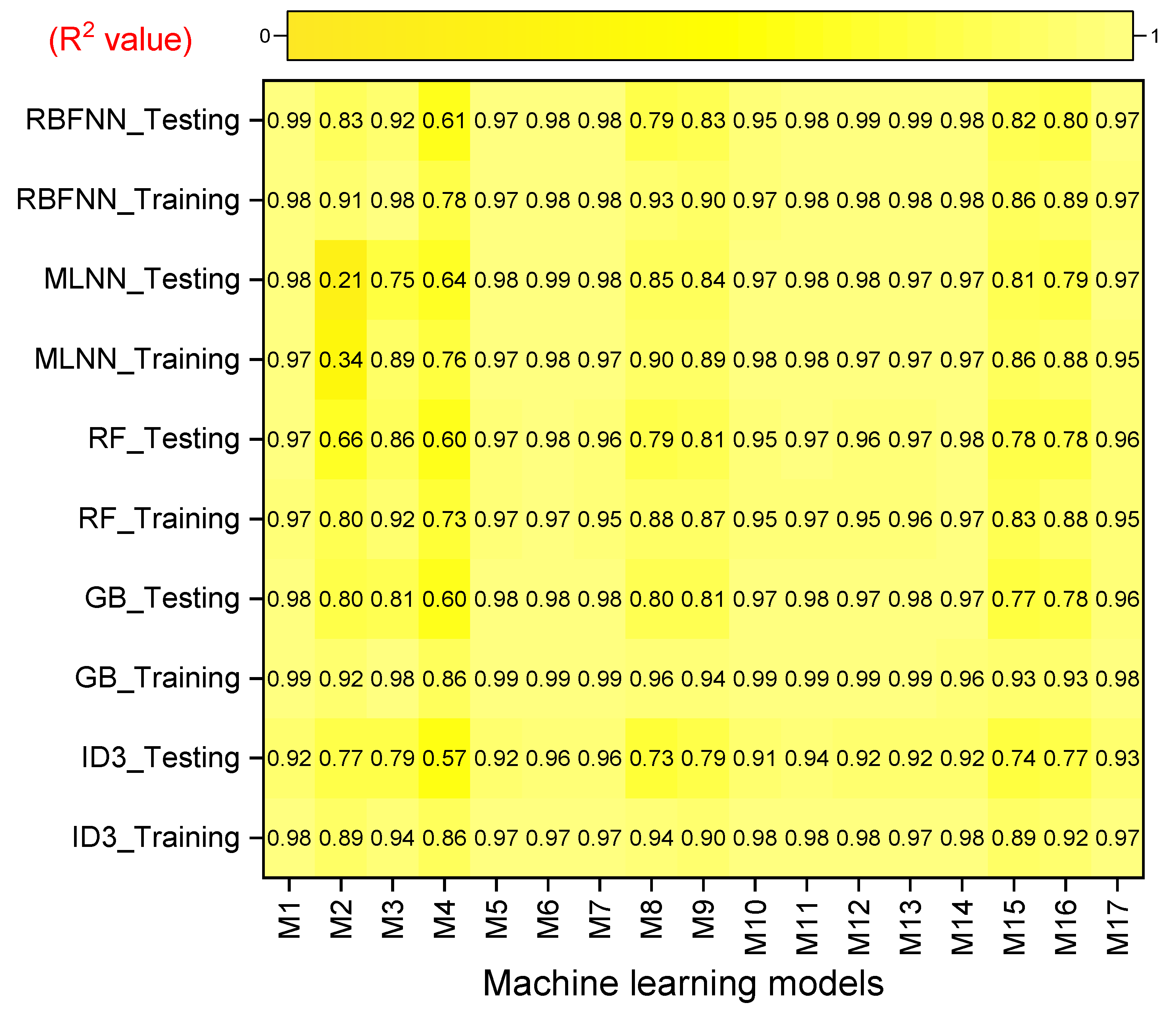
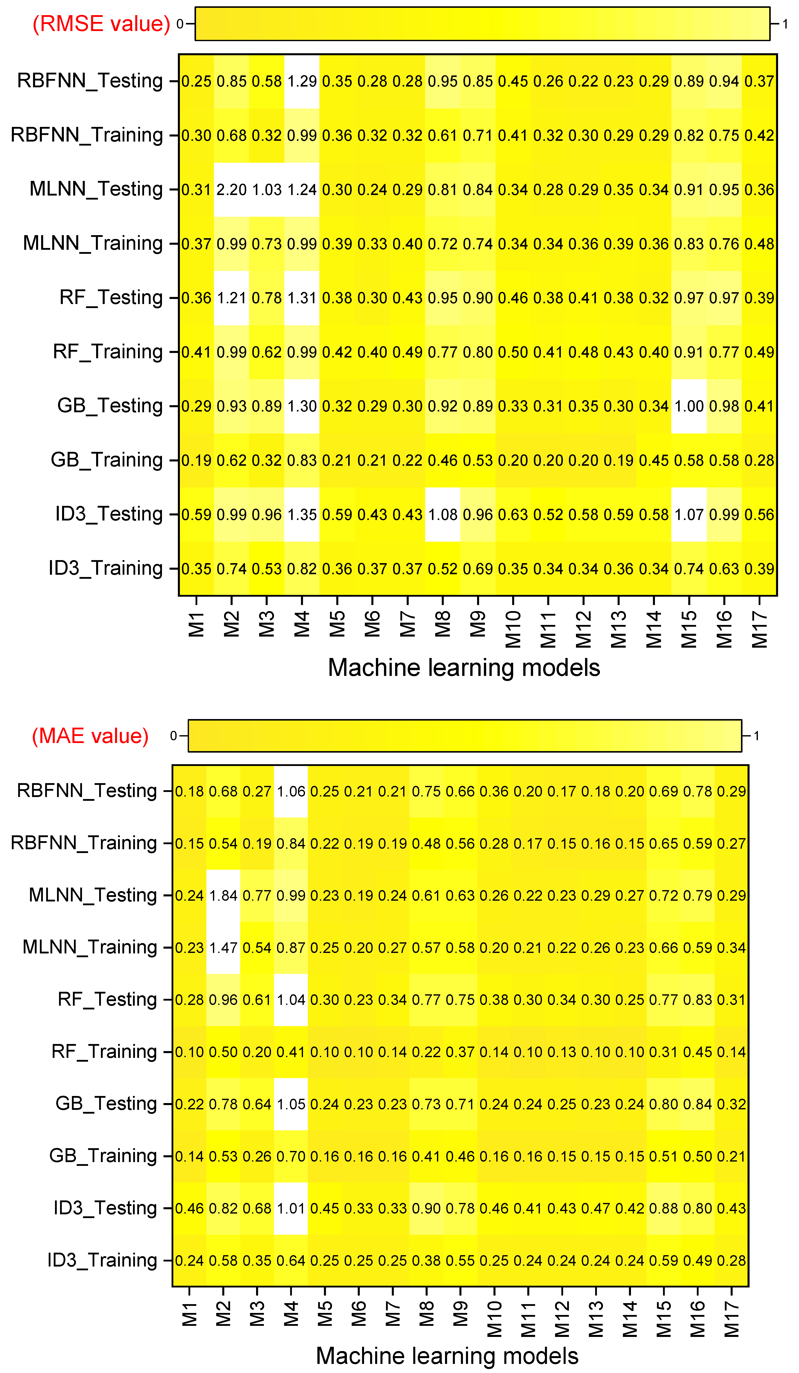
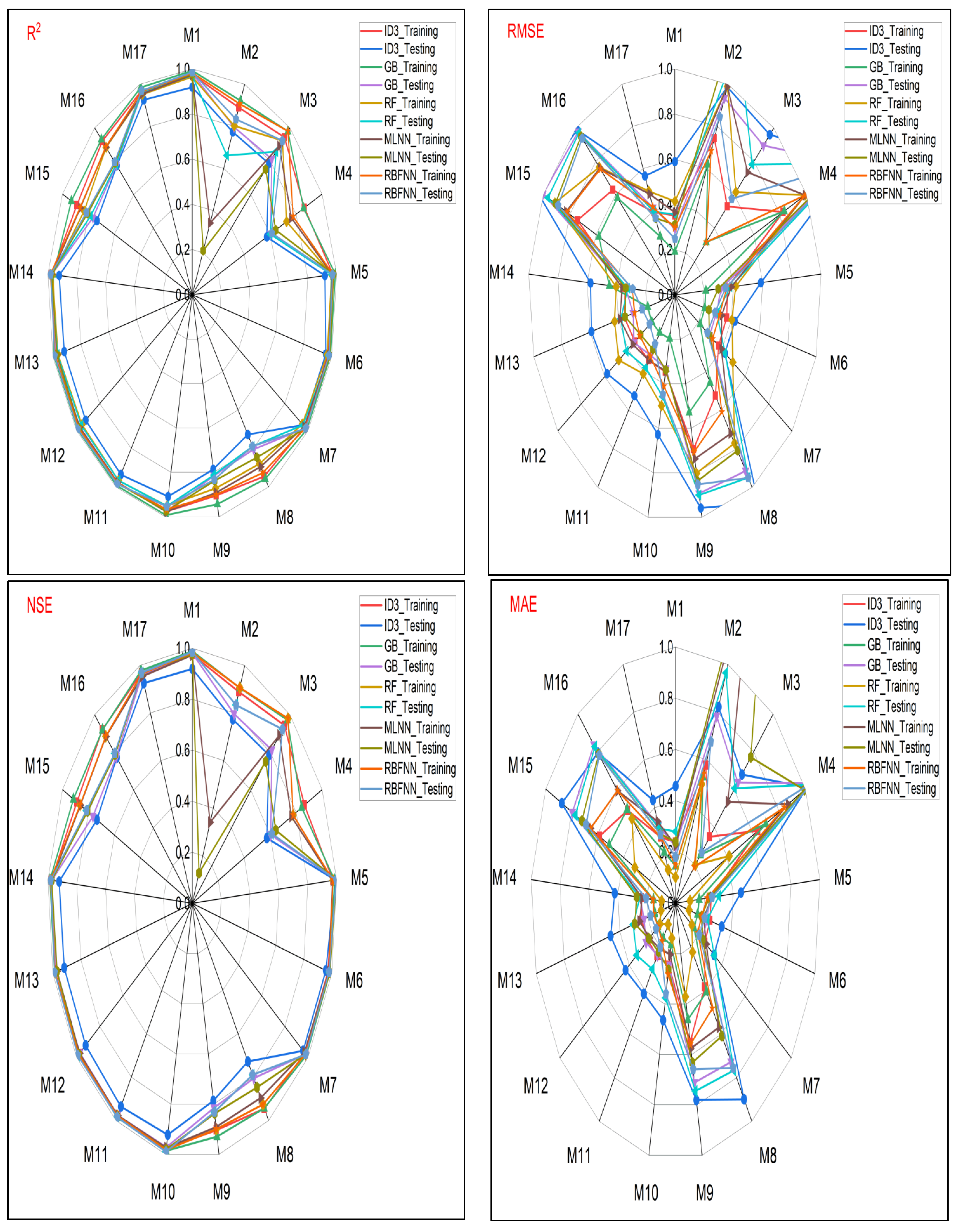
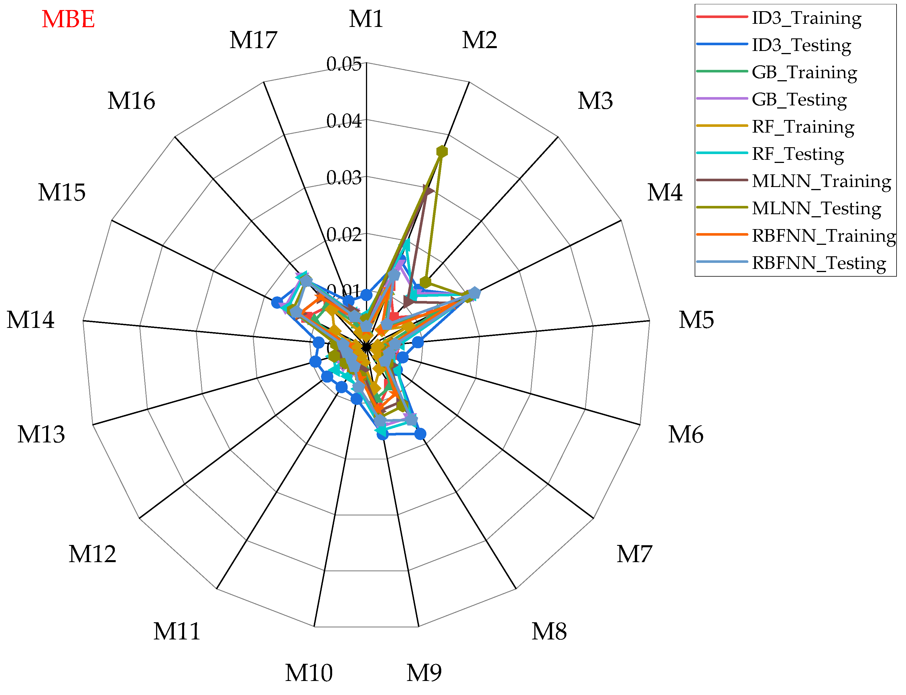
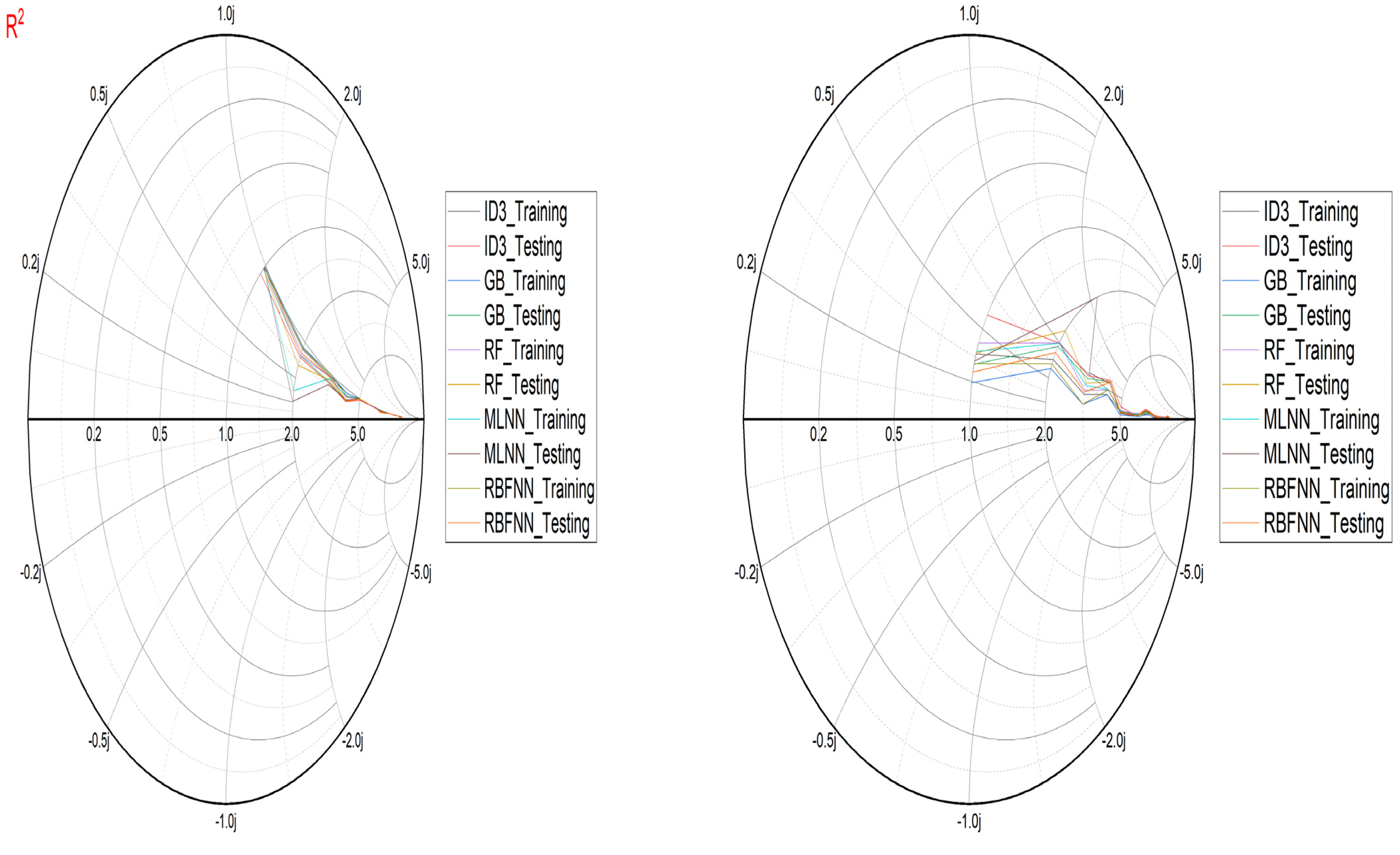
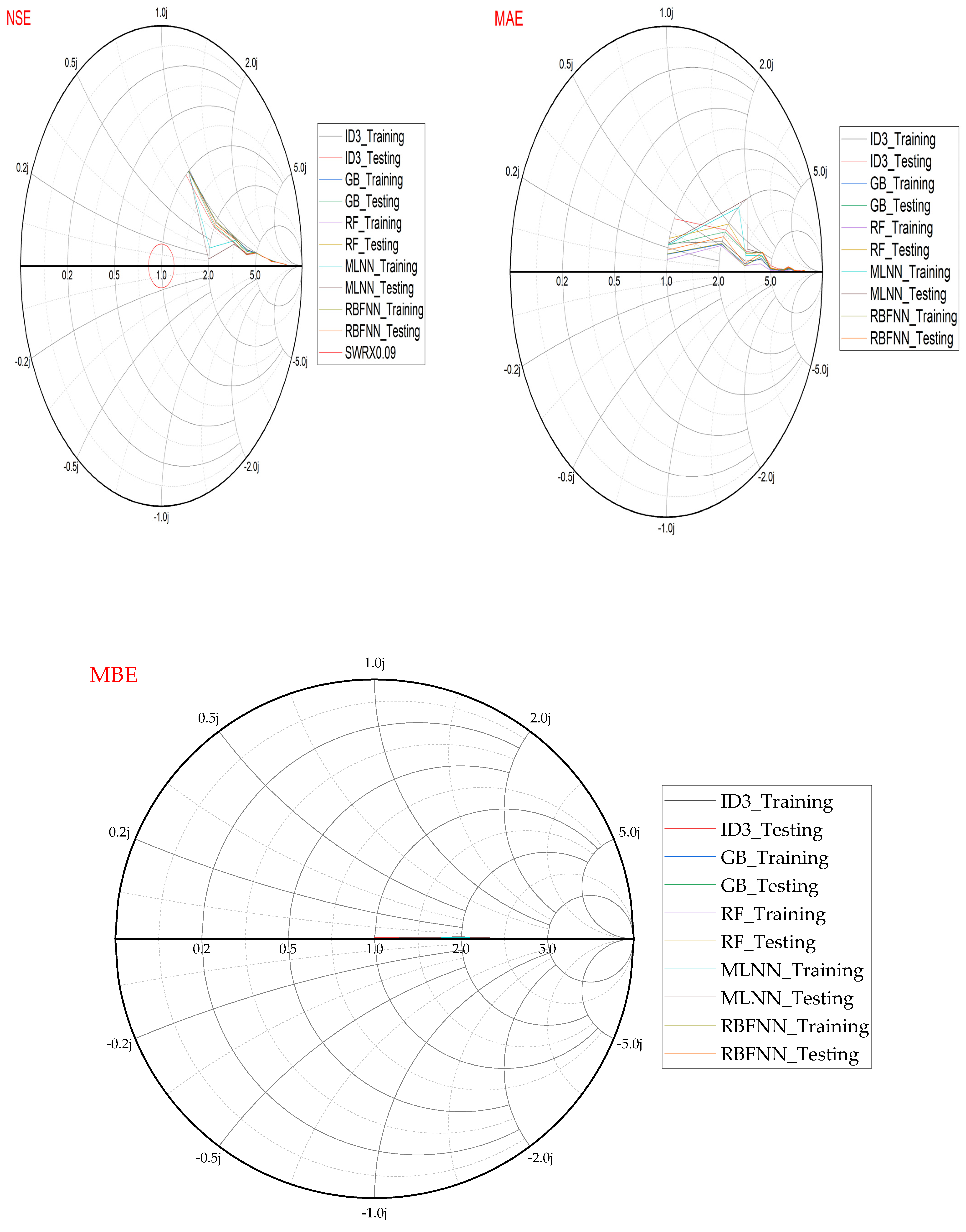
  • Performance evaluation of ML algorithms through visualization (radar, heatmap, bullet, and Smith graphs) based on different statistical indices to determine the best one among them.
The findings of the current study practically contributed in a way that the ETo retrieved from the ML model may be interpolated into monthly and yearly ETo maps depicting ETo variations over the studied area. Agronomists, hydrologists, and agricultural engineers may use the ETo maps to more accurately determine the water needed to irrigate the crops (via drip and spray irrigation).

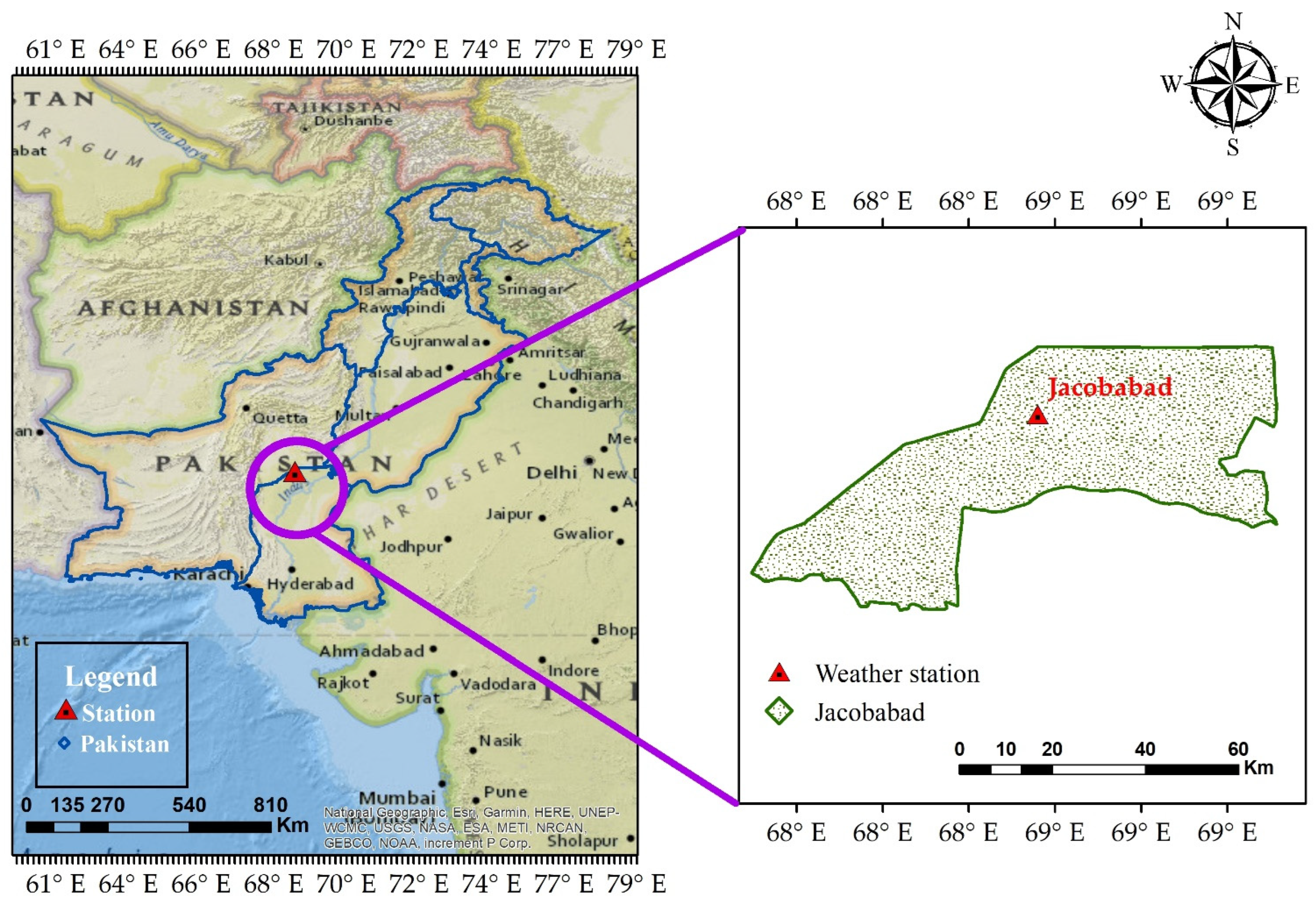
2. Study Area and Dataset

Pakistan lies between moderate to scorching climatic zones [52]. Temperatures vary widely from location to location, but the climate is generally arid, with scorching summers and frigid winters. The current study obtained climatic data of Jacobabad Meteorological Observatory (JMO) from the Regional Meteorological Center (RMC) Karachi (weblink: https://rmcsindh.pmd.gov.pk/, accessed on date 15 August 2023). The observatory (index number 41715) installed by the RMC is situated at a latitude of 28°18′, longitude of 68°28′, and altitude of 56 m (Figure 1). Table 1 displays a summary of 30 years (1987–2016) of climatic variables obtained from the RMC. Furthermore, Figure 2a,b present monthly and interannual changes in the climatic variables utilized in the present study. Figure 2a shows a notable trend wherein the minimum temperature (Tmin) exhibited an initial increase from January to July, followed by a slow decline until December. The observed pattern in Tmax was consistent, as shown in Figure 2a. The fluctuation in seasons can be attributed to the solar radiation emitted by the sun, as depicted in Figure 2a. Sh witnessed the summer’s peak and the beginning of winter’s decline. The variable RHmean exhibited a relationship with both Tmax and Tmin, as it was seen that the periods of elevated air temperature coincided with the highest levels of humidity. According to the data presented in Figure 2a, the average relative humidity (RHmean) exhibited its maximum values throughout July to September, which can be attributed to the impact of wind, and there could be much more important meteorological reasons, such as the atmospheric circulation pattern together with the surrounding ocean and topography of the selected regions. During the summer season, it can be observed from Figure 2a that there is an upward trend between wind speed and humidity levels in the air. The summer months exhibited the most notable rise in average and maximum humidity levels. In addition, Figure 2b indicates cyclical conditions of climatic variables starting from 1 January to 31 December for the years 1987 to 2016.

Physical–Geographical Conditions

Jacobabad is geographically situated in a manner that it shares its boundaries with three provinces concurrently. These provinces include the Rajanpur District of Punjab Province and the Nasirabad district of Balochistan Province. The Indus River influences the district, resulting in direct effects on the Kashmore and Kandhkote Tehsils. The Guddu Barrage in the Kashmore Tehsil serves as the point of origination for historical water channels, such as the Pat feeder canal. The total land area of Jacobabad district is 2686 square kilometers. The district encompasses Kacha communities residing in the Kandhkote and Kashmore Talukas, occupying extensive land parcels on both banks of the Indus River. The agricultural output of the Kacha region is limited to Rabi crops due to the annual flooding of the river during the summer. The investigated site exhibits varied topography and variations in elevation, resulting in significant variations in evapotranspiration values. The gradual decrease in elevation from Kashmore to Jacobabad and its surrounding areas has not obstructed the river’s continuous flow. The Indus River has facilitated social and agricultural development by watering and feeding the surrounding landscape, enabling the cultivation of crops twice a year without the need for fallow periods. During the Kharif season, most of the paddy is harvested and rabbit crop wheat is sown, both of which need a lot of water. Nevertheless, the issues of floods and salinization have emerged as significant challenges, resulting in detrimental effects on agricultural land and a decline in crop productivity. Attempts to mitigate the prevailing circumstances involve implementing drainage systems and excavation activities aimed at reducing the water table. However, despite such efforts, the situation continues to progressively deteriorate. The management of sewage systems is a prevalent concern across the western bank, necessitating the implementation of a siphon mechanism to divert the flow of wastewater towards the left bank.

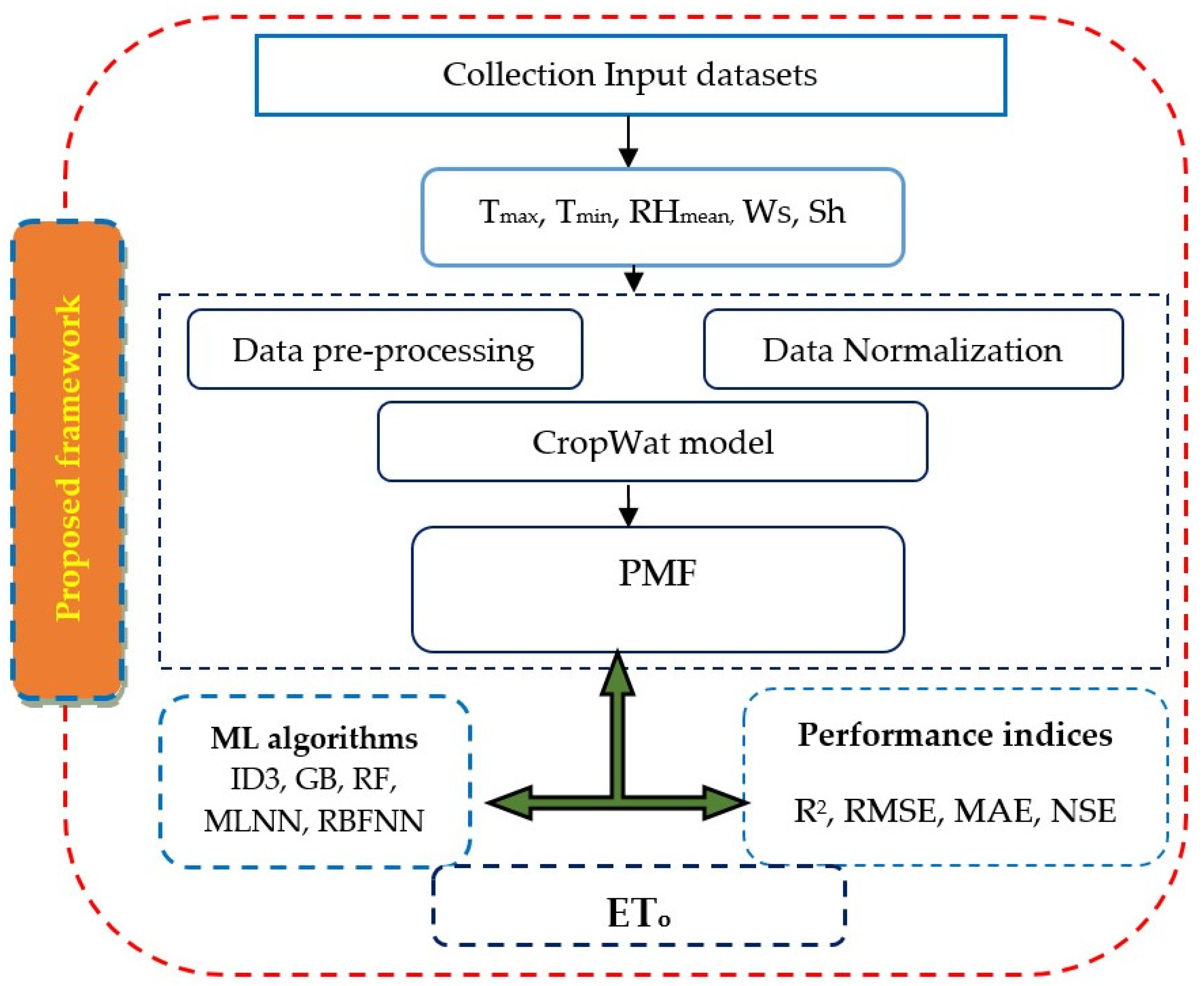
3. Study Methodology

3.1. PMF

The CROPWAT software version 8.0 from the FAO of the United Nations was used to compute the ETo using meteorological input values. The PMF approach was used to determine the value of ETo in this software (Weblink: https://www.fao.org/land-water/databases-and-software/cropwat/en/, access date, 20 September 2023). The PMF developed by Allen et al. [4] in 1998 determines ETo values based on a combination of meteorological and aerodynamic parameters (es, ea, emin, emax, Δ, G, and Ɣ). The mathematical notation of the PMF is described as follows:
E T o = 0.408 R n G + γ × 900 T m e a n + 273 × W s × e s e a + Ɣ 1 + 0.34 W s
where:
ETo is measured in mm/day; Rn = net radiation at the surface (MJ/m2/day);
G = soil heat flux density (MJ/m2/day); Tmean = air temperature at 2 m height (°C);
es = saturation vapor pressure (kPa); ea = actual vapor pressure (kPa);
Δ = slope of vapor pressure curve (kPa/°C); γ = psychrometric constant (kPa/°C);
Ɣ = 0.000665 × p (kpa); es is saturation vapor pressure (kPa); Ws = wind speed.

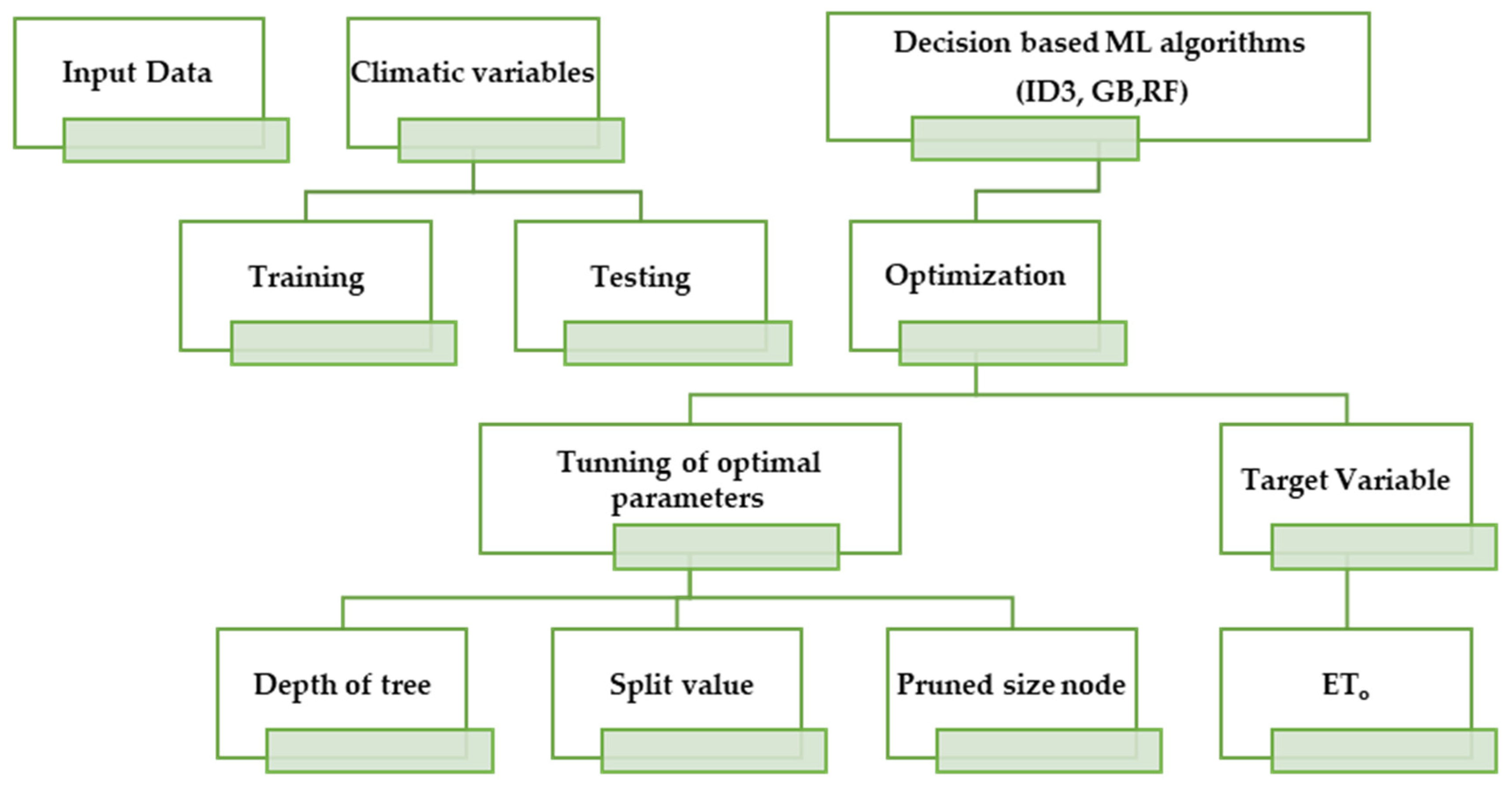
3.2. Proposed ML Framework

PMF ETo was used as the benchmark for output (ETo) values when chosen ML algorithms were applied. For this purpose, we used Waikato Environment for Knowledge Analysis (WEKA) software version 3.9.4. It is a collection of machine learning algorithms for data mining tasks. It contains tools for data preparation, classification, regression, clustering, association rules mining, and visualization. It is an open-source software issued under the GNU General Public License (weblink: https://www.cs.waikato.ac.nz/ml/weka/, accessed date, 5 August 2023). Weka was used in this study, and the following steps were implemented. The dataset used was pre-processed in the first step (1). The data file was prepared in comma-separated values (CSV) file format (2), and it was uploaded to Weka software by using the import feature (3). The optimal parameters related to ML algorithms were selected (4), data were classified (5), and the nearest neighbor was chosen as the estimation function (6). In the cross-validation process, K-means clustering was utilized (7), association rules were performed (8), and, in the last step, the model was evaluated (9). A schematic framework of the ML models suggested for ETo estimation is shown in Figure 3.

3.2.1. Iterative Dichotomizer (ID3)

The ID3 algorithm relies heavily on the measurement of entropy and information gain. Both entropy (E) and information gain (IG) may be defined in terms of the predicted decrease in entropy (Purity) and the homogeneity (H) of a learning set (Impurity), respectively. E and IG may be written in general mathematical form using Equations (2) and (3), respectively. If p is the fraction of S in class i, then both terms are provided by Equations (4) and (5) in the discrete case.
E = A log 2 A B log 2 B
I G = S b S a
( E ) b = i = 1 k p i log 2 p i
( I G ) b = i = 1 k p i 2
where Sb is the entropy of distribution before the split, Sa is the entropy of distribution after the split, (E)b is the entropy for the k-wise classified function, and (IG)b is the information gain for the k-wise classified function.
The decision model may benefit significantly from simplification by following the top-down greedy (TDG) search process. The TDG process is straightforward and consists mainly of two parts. Using the provided data, initial calculations for each characteristic are made. Second, we determine a function that optimally divides the node. The TDG procedure and the depth of the resulting tree are also critical factors in the categorization of datasets. The ideal value of each characteristic is evaluated and then used to divide the tree node. The E and IG are then compared for each characteristic. The property with the highest IG and lowest E value is chosen as the root node’s primary identifier. IG aims to create a hierarchy in which attributes are ranked from top to bottom, starting at the root node. There is currently insufficient evidence to conclude that the attribute present in each node with a greater value of IG and a lesser value of E is adequate to establish a root node. This hierarchy aims to facilitate the desired moderation of the decision-making process. As a result, we created a forest of little trees with shallow roots. A smaller tree facilitates faster dataset identification. We chose the attribute with the highest E and IG values from the training data and assigned it to the root node. We created smaller subsets of the training data that were assembled into a larger whole. Each attribute value should be consistent across all datasets used to create the subset. Recursion happens until a child node has been formed for each branch. Ultimately, we compared the recorded attribute values to the original attribute.

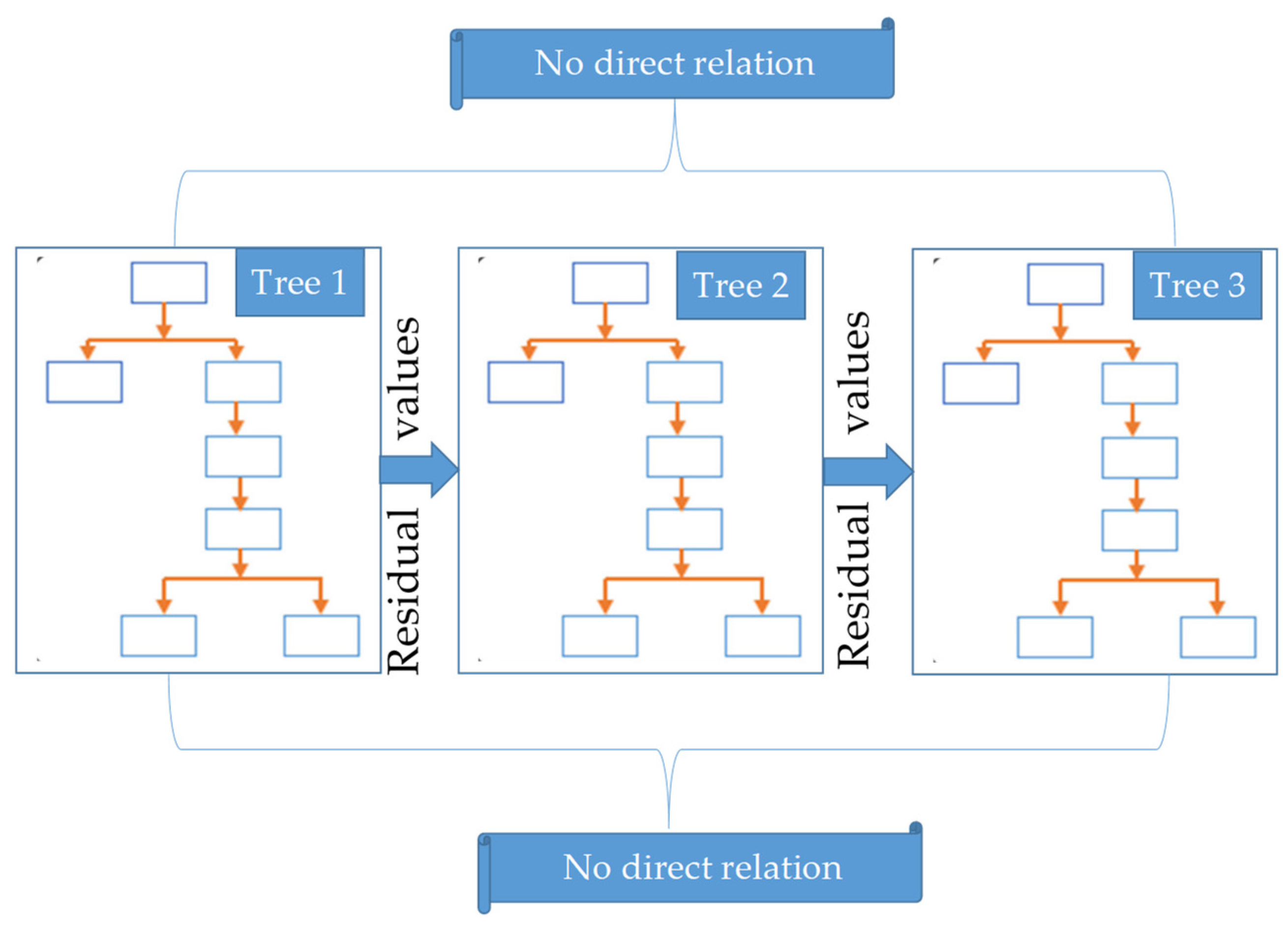
3.2.2. Gradient Boosting (GB)

Gradient boosting is a method through which a prediction function is increased by repeated use. After that, we add each function’s output according to its relative importance. By taking this measure, prediction will get closer to accuracy, and errors will be eradicated. Because of this helpful property, GB is often represented as a linear model. The ability of this approach to decouple dependent and independent variables is a significant plus. Equation (6) is a numeric representation of the GB model, and it is written as
predicted target = Fo + B1 × T1 (X) + B2 × T2 (X)………………+ Bm × Tm (X)
where Fo is the starting value in the series, X is the vector of “pseudo-residual” values remaining at this point in the series, Tx(X) represents the trees fitted to the pseudo-residuals (here, x = 1, 2, 3…….m), Bx is the coefficient of the tree node predicted values (here, x = 1, 2, 3…….m).
The boosting procedure will use a primary tree ensemble mechanism, as seen in Figure 4. It has been discovered that a succession of three trees is connected. Tree 2 receives the residual values that Tree 1 produces. Likewise, the values of Tree 2’s residuals may be found in Tree 3’s structure. Furthermore, there is no apparent connection between Trees 1 and 3. This procedure was repeated until every relevant data subset was included in the phase. Next, the weighting index of each tree is added to the dataset, and the misclassification error is calculated.
There are several ID3-style trees inside a GB ML algorithm. Each of these supplementary trees is connected to the others. Thus, there is a link between the neighboring trees. So, it is a chain of trees connected. In this investigation, we explored the following applications of the GB algorithm: (i) The climate predictor variables and their corresponding input parameters. (ii) Misclassification errors that occurred during model calibration were eliminated using the Huber loss function and the surrogate splitter technique. The K-type classification was employed for dataset segregation, partitioning it into k and k−1 subsets. Following multiple trials and an error-based approach, tree numbers for the GB model at minimum and maximum level were allocated to create a series that enables ensemble processing. The k-test subsets were thoroughly tested, with the k-1 subset serving as a means for instruction. The overall ETo value was predicted by averaging the values from the various subsets.

3.2.3. Random Forest (RF)

The bagging technique is a collection of untrained decision trees utilizing bootstrap samples. The underlying structure of the method used to build the RF model may be grasped quickly. Treat the whole dataset as if it were N observations. Select the desired subset of N observations from the data collection. Bagging is the term for this operation. Some observations are utilized many times in the bagging process. Thus, not all of them are included in the analysis. Two-thirds of a data collection is often sampled, with the other third classified as “out of bag” (OOB) information. Each tree is built using a random subset of the available data.
The data from the chosen rows are then used to construct a decision tree. It is intriguing to learn that, unlike the ID3 and GB models, the RF model does not need tree pruning. The bagging procedure is performed recursively until all trees have been built. Only a subset of the available predictor variables is used when building a tree. Each node’s potential splitter is chosen randomly from this collection of predictor factors. For instance, if there are six predictor variables, three will be selected randomly to be used as splitter candidates.
Nonetheless, the uninvolved variables might be utilized for another node split in the same tree. Not all of the predictor variables have to be used in the separation. Thus, some predictor variables may need to be used throughout a tree’s structure. This procedure is repeated until a wooded area has been established. After a subset has been chosen, the scoring process involves cycling over each tree in the forest in turn with each data row. The scoring method generates projected values that are used in the development of terminal nodes. Using several techniques, the RF model yields accurate predictions in regression and classification analyses. When doing a regression analysis, the typical score predicted by all trees is determined. The “votes” for the best variable in a classification study come from the variables predicted for each tree. The most popular predictor variable is used to provide a score for each row in the tree. There are two forms of randomness in an RF algorithm. First, a subset of rows from the data is used as an input for each tree, and then a predictor variable is utilized to determine how to divide up the nodes in the tree. These supplementary characteristics significantly boost the RF model’s overall predictive accuracy when added to forecasts. The following procedures were used to create the TF model for this investigation:
  • Climatic variables were chosen as predictors/inputs.
  • The sample data constituted 70% of the total dataset, separated using the randomization function.
  • Analysis was performed using dataset (OOB), and residual values were stored separately.
  • The ETo obtained from each tree as output was gathered and stored.
  • The mean values of the output variable (ETo) were computed as a whole.
Figure 5 shows the procedure for using ML algorithms that make decisions. As a starting point, we feed in data on temperature ranges, humidity averages, wind speeds, and sunshine totals. Separate sets of data, known as train and testing, were created. Second, we tuned ideal parameters to improve the performance of the ID3, GB, and RF algorithms used to calculate ETo. Table 2 overviews the best possible ID3, GB, and RF parameters.

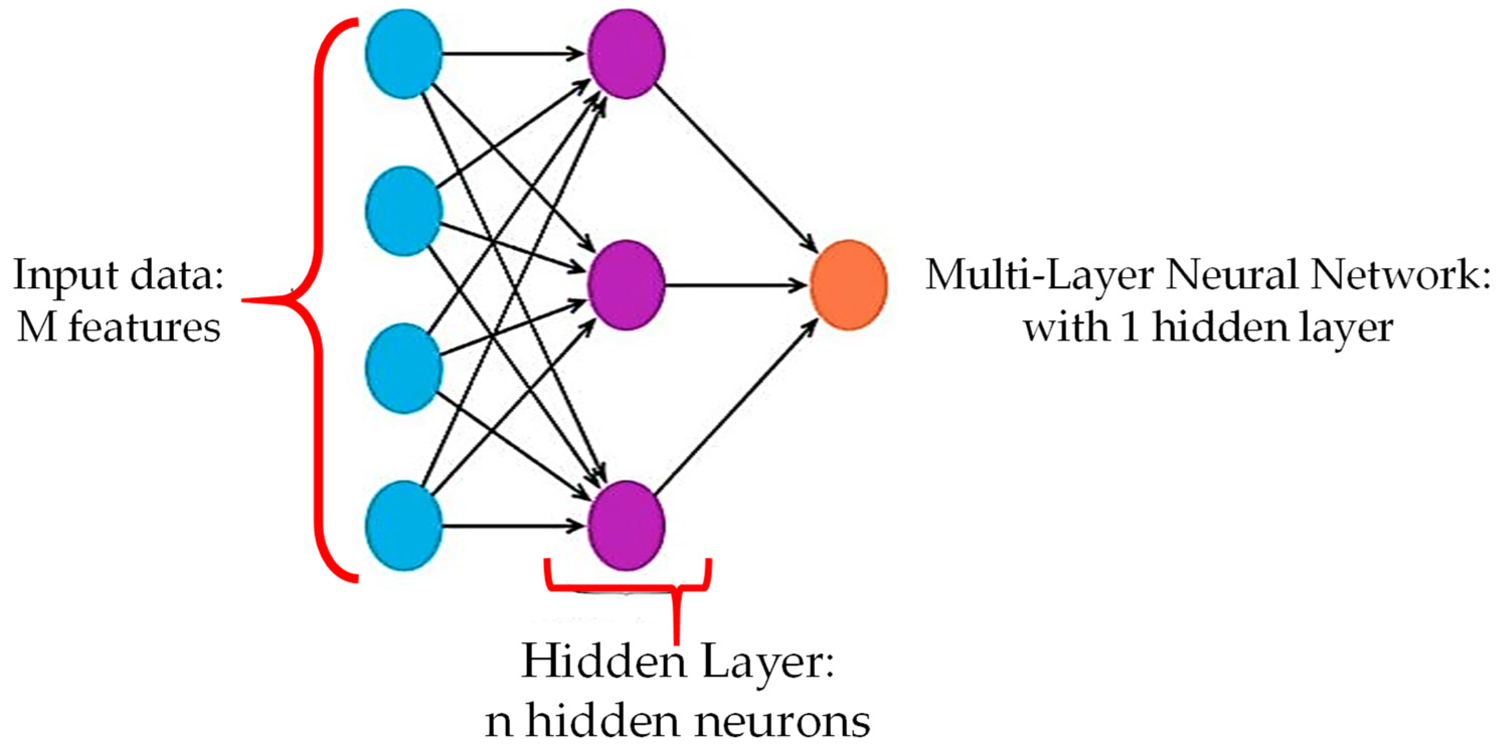
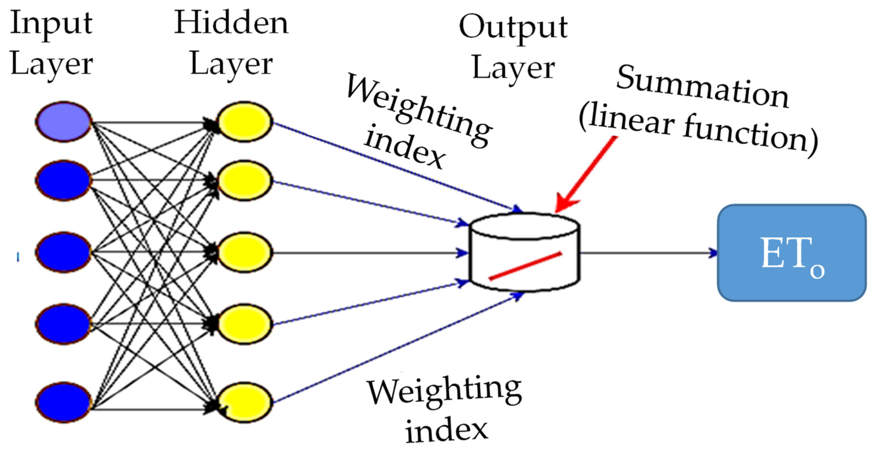
3.2.4. Multilayer Neural Network (MLNN)

An input layer, a hidden layer, and an output layer make up the MLNN architecture. There are a certain number of neurons in each layer, all of which communicate in the same way. Predictor variables from the previous layer are stored in each neuron, as are the number of outputs to the next layer. The structure’s overall effectiveness depends on the contributions of each layer. Weights establish the precise nature of the connections between neurons in different layers. The results are supposed to be carried by these kilos from one layer to the next. Each neuron in the input layer sends its output to a corresponding neuron in the hidden layer. Just as the output of one neuron in the hidden layer becomes the input of another neuron in the output layer, the reverse occurs in the output layer. Figure 6 depicts an MLNN architecture with a single hidden layer. The input layer neurons are all linked to one another in the hidden layer, while the hidden layer neurons are only linked to one another in the output layer. Input and output layers do not have any “direct” connections between their neurons. The name “feed-forward neural network model” comes from the unidirectional nature of the data flow it facilitates. The following procedures were used to determine ETo using the MLNN:
  • Climate-related input variables were chosen as predictors.
  • Sigmoid and linear activation functions were used in the input-hidden and hidden-output layers.
  • The weight connection between interconnected neurons was adjusted via the adoption of a back-propagation procedure.
  • The kernel functions utilized were Traditional Conjugate Gradient (TCG) and Scaled Conjugate Gradient (SCG).
  • The ETo was estimated as an output.

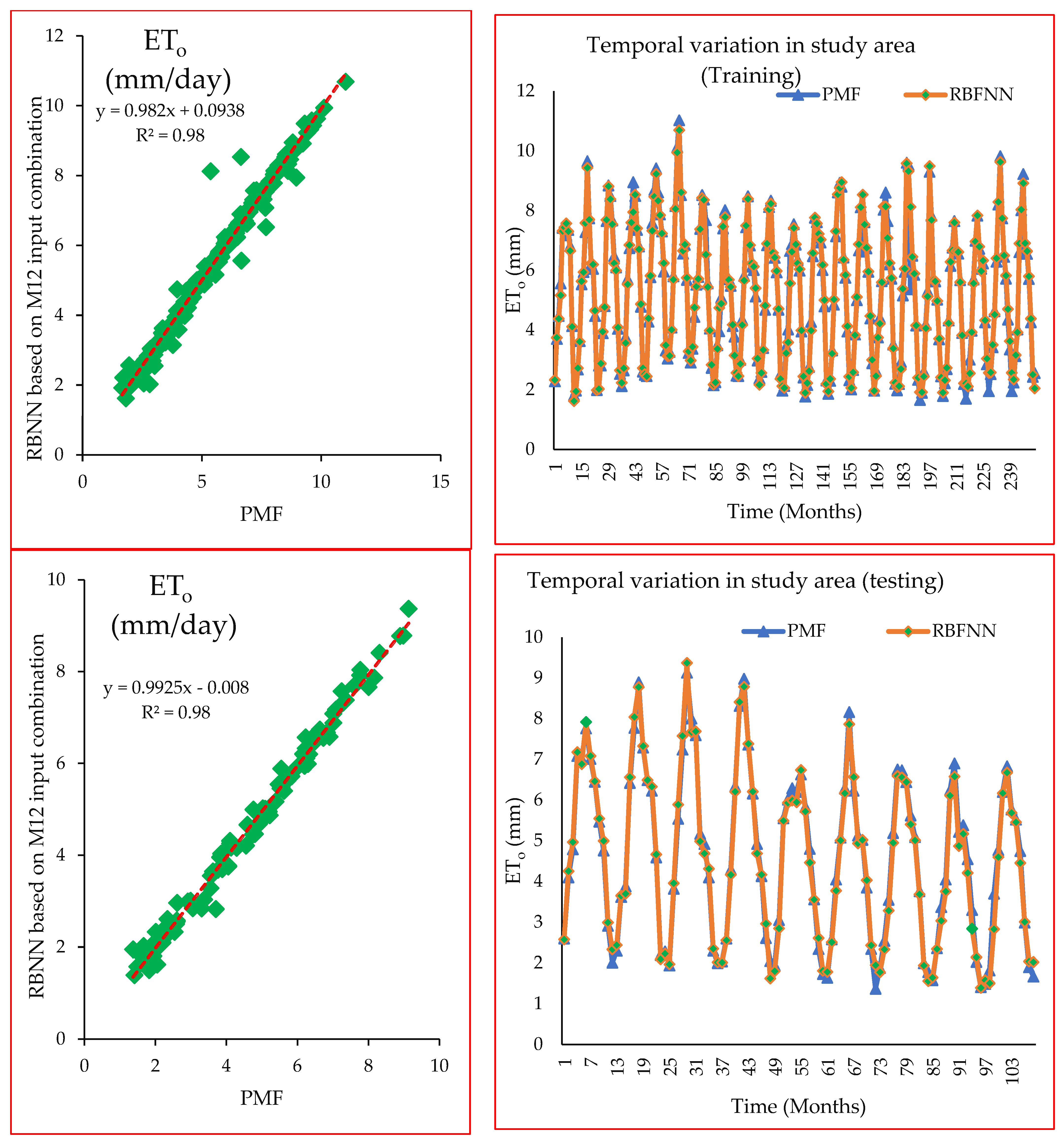
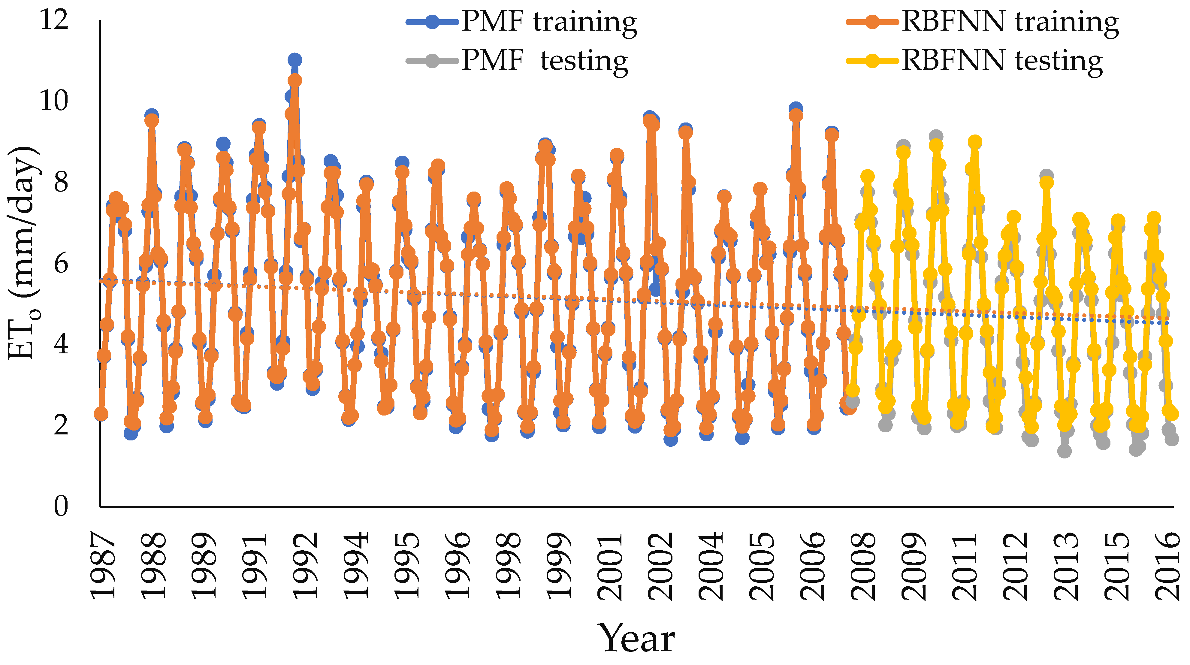
3.2.5. Radial Basis Function Neural Network (RBFNN)

There are three distinct layers in the RBFNN: the input, the hidden, and the output. Simply put, the input layer is made up of a large number of neurons that are linked to the hidden layer through weighted connections. These weights convey the values from one layer to the next. The input layer neurons utterly unconnected to one another form the output layer. Both a hidden layer and an output layer need linear and transfer functions. Activation functions are another term for these mathematical operations. A parametric vector accompanies the neurons in the buried layer. This vector, known as the hidden layer’s center, may be considered a weighted index. The distance between an input vector and the hidden layer’s center is quantified using the Euclidean distance (E). The RBFNN network used in this analysis was developed as follows. We used V-fold cross-validation to ensure the integrity of the dataset, tuned the RBFNN network to optimal performance by selecting a population size of 200 and a maximum generation of 20, and used the radial basis function’s activation function in both the hidden and output layers. Figure 7 depicts a schematic representation of the RBFNN algorithm used in this investigation, illustrating the input–output link between climate variables and ETo.

3.2.6. Selection of Meteorological Input Combinations

A total of 17 meteorological input combinations were used as input, which are tabulated in Table 3. It can be perceived that M1 contains inputs Tmin, Tmax, RHmean, Ws, and Sh for ETo estimation. When M2 is used to estimate ETo, ML algorithms (ID3, GB, RF, MLNN, and RBFNN) with the RHmean and Sh variables are considered as inputs. Likewise, Table 3 provides information on the other 15 input combinations (M1 through M17) in the same format as M1 and M2. Previous research evaluated the performance of the ML algorithms using various statistical criteria [40,41,42,43,44,45,46,47,48,49,50]. The ML algorithms’ performance using all 17 input combinations was measured using the statistical indices root-mean-square error (RMSE), determination coefficient (R2), mean absolute error (MAE), mean bias error (MBE), and Nash–Sutcliffe efficiency (NSE).
R 2 = i = 1 n E T o b s E T o b s ¯ E T e s t E T e s t ¯ i = 1 n E T o b s E T o b s ¯ 2 i = 1 n E T e s t E T e s t ¯ 2 2
R M S E = i = 1 N ( E T o b s E T e s t ) 2 n
M A E = i = 1 N | E T o b s E T e s t | n
N S E = 1 i = 1 n ( E T o b s E T e s t ) i = 1 n ( E T o b s E T o b s ¯ )
M B E = 1 n i = 1 n ( E T o b s E T e s t )  
where ETobs, ETest, E T o b s   ¯ , and  E T e s t ¯ are the observed, estimated, average observed, and average estimated ETo, respectively, and n represents total records.
R2 is the goodness-of-fit parameter, which may be from 0 to 1. It is a number between −1 and 1 that has no dimensions. A correlation coefficient near 1 indicates a strong association. The MSE calculates the average squared deviation between observed and anticipated values. When comparing errors between experimental and anticipated values, the root-mean-square error (RMSE) is often utilized. Model performance improves when the MSE, RMSE, and NRMSE values decrease. The NSE index is a regularly used goodness of fit statistic to evaluate a model’s effectiveness. The NSE may be measured from −1 to 1. Lower RMSE and MAE values and greater R2 and NSE values indicate a superior model.

4. Study Results

Figure 8, Figure 9, Figure 10 and Figure 11 show the findings as several statistical indices (RMSE, R2, MAE, and NSE). The 30-year, 360-record dataset was split into training (252 records) and testing sets (108 records). Each ML model’s performance accuracy over all seventeen scenarios was evaluated using the testing set. The training set was utilized for calibration and model development. The ETo estimated with the PMF was used as the standard for assessment of both decision-based and neural network-based ML algorithms.
The study considered various meteorological variables’ possible combinations (M1 = Tmin, Tmax, RHmean, Ws, Sh to M17 = Tmean, Ws) to determine their impact on ETo prediction. The performance of ETo prediction was evaluated by adding and removing different meteorological variables. The interpretation of the performances was based on a combination of statistical indicators and graphical approaches. Figure 8 presents the performance evaluation of ML models using bullet charts. The structure of statistical metrics for each model in the training and testing phases is provided. It is worth mentioning that all the ML models created attained high levels of accuracy. Nevertheless, after scrutinizing the NSE and R2 values, it can be deduced that the RBFNN algorithms and the M12 and M13 combinations showed the highest precision. Likewise, examining the RMSE and MAE values, it was concluded that the M12 combination exhibited the lowest error rate and yielded the most precise prediction results using the RBFNN ML algorithms.
In Figure 9, the selection of the optimal ML model is evaluated through performance metrics and addressed with heatmap representations. Different data densities represent different levels of relationship and measurement. The combinations M1, M5, M6, M7, M10, M11, M12, M13, and M14 exhibit similar and satisfactory levels of prediction accuracy based on R2 and NSE values. However, the highest prediction for ETo was achieved using RBFFNN algorithms. When evaluating ML model performances based on RMSE and MAE error metrics, the suitable input combination was found to be M12. Additionally, the model combinations M1, M11, M12, and M13 stand out for their low RMSE and MAE and high accuracy (NSE and R2) as compared with other input combinations. Furthermore, when the optimal algorithm is considered, the RBFNN algorithm was tested to yield the highest prediction performance. According to this, the optimal model has RMSE values of 0.30 during training and 0.22 during testing. Additionally, the MAE values for this model are 0.15 during training and 0.17 during testing. When examining the R2 and NSE values, they were observed to be 0.98 during the training phase and 0.99 during the testing phase.
Figure 10 shows the performance evaluation of the ML models for ETo prediction using radar charts. When evaluating the R2 and NSE values, it is observed that the models M1, M5, M6, M7, M11, M12, M13, and M14 exhibit high prediction accuracy, with the RBFNN algorithm achieving the highest accuracy. The GB algorithm is also successful as a second-degree model. On the other hand, the highest error (RMSE and MAE) was obtained with the ID3 algorithm. When performing a performance analysis based on RMSE values to determine the optimal model for ETo prediction, the RBFNN model emerges as the model with the lowest error. The second-best ML model is identified as GB, followed by GB and ID3. Additionally, analyzing the MAE values reveals that the algorithm with the lowest error is the RBFNN, while the second-best ML model was RF, followed by GB and ID3. Overall, RMSE and MAE obtained the highest in the case of ID3 ML algorithms.
Input and output values may be visually converted using a Smith chart. A planar grid is constructed for this purpose, allowing the output value to be calculated for a particular input. The Smith Chart is only a plane with circles superimposed on top to determine the results of each independent variable. In Figure 11, the Smith chart further supports the abovementioned results and explains the efficiency (R2, NSE) and error (MAE, RMSE) of the applied ML models. The Smith chart is a particular kind of impedance chart that has parallel series of lines. Lines in the first set, called constant resistance lines, display mutual tangency along the right side of the horizontal diameter and form circles. Constant resistance (j) circles are the conventional name for these spherical formations. The values of the resistances represented by the j circles are shown on the horizontal diameter where the circles connect with the line. The circle of positive resistance is shown on the top side of the horizontal line, while the circle of negative resistance is shown on the bottom side of the horizontal line. It is observed in Figure 10 that statistical indices (R2, NSE, MAE, and RMSE) of the ML models lie on the top side of the horizontal line, which corresponds to the positive value ranging between 0 and 1. In addition, it was noted that the RBFNN approaches 1 for R2 and NSE while MAE and RMSE decline to 0, indicating the superior performance of the RBFNN as compared with other applied ML models.
Figure 12 shows a scatter plot and temporal variation by comparing ETo estimated with the RBFNN using the M12 input combination (best model) and standardized PMF in the training and testing phases over the studied region. It is clearly observed in Figure 11 that RBNN trailed well with the PMF and could be used in cases of limited climatic input data. In addition, Figure 13 indicates temporal variation in ETo estimated with the RBFNN and PMF from 1986 to 2016 in the training and testing phases. It can be concluded that the RBFNN algorithms performed well and coincide with the ETo values of the PMF.
In addition, the MBE captures the average deviations between two datasets. It has the units of the variable. Values near 0 are the best; negative values indicate underestimation and positive values indicate overestimation. Moreover, RMSE combines the spread of individual errors. Figure 8, Figure 9, Figure 10 and Figure 11 indicate that the MBE produced by ML models at all the 17 input climatic combinations found nearly zero, which indicated the superior performance of the chosen ML models. The results also affirmed the use of ML models in cases of limited climatic data because there is no underestimation and overestimation found in the dataset. It can also be confirmed that the dataset used in the current study has no missing values and no abnormality was detected during data analysis.

5. Study Discussion

Within the scope of the presented study, various machine learning models were evaluated to the peak for the estimation of ETo values. Accordingly, the RBFFNN model had the highest accuracy and ID3 showed the weakest prediction success. It was deduced that the Tmean, RHmean, and Ws input variables had the highest effect on ETo estimation. Pal and Deswal [57] employed the M5 model tree method to model daily ETo in the climatic data of Davis station, which California maintains. The inputs for the model were solar radiation, average air temperature, average relative humidity, and average wind speed. The M5 model tree model successfully predicted meteorological data and ETo values, as evidenced by the results of this research. The outputs of this research support the presented study. The study conducted by Vaz et al. [58] employed machine learning and deep neural networks to construct a model for evapotranspiration, utilizing only a limited number of weather variables, including temperature, humidity, and wind. The presented research coincides with this research, as both establish the Random forest algorithm’s potential to provide satisfactory outputs for ETo estimation. Also, LSTM-ANN recommends a hybrid approach for ETo estimation. The estimation of ETo has been predicted by Wang et al. [59] through the utilization of a combination of time granulation computing techniques and gradient boosting decision tree (GBDT) with Bayesian optimization (BO). Subsequently, GBDT is deployed to anticipate evapotranspiration, while BO determines the optimum hyperparameter values from the pared-down granules. The study’s findings align with current research, indicating that the GB algorithm substantiates the sufficiency of ET prediction. The effectiveness of various types of ML algorithms, including tree-based, neural network-based, multifunction-based algorithms, and a combination of ML and physical models, have been investigated in predicting hydrological variables (ETo, river discharge, precipitation, monitoring droughts) and their related factors [60,61,62,63,64,65,66,67,68,69,70,71,72,73,74]. Wang et al. [59] analyzed temperature data from several different climatic stations located in Pakistan [60]. The TB model produced outperforming results (R2 and NSE = 1.00, MAE and RMSE = 0.26 and 0.37) when an input combination based only on temperatures (Tmax and Tmin) was used. The study’s outputs support the current study in terms of tree-based algorithms showing high performance in ETo model estimation. However, ETo estimation established only with the maximum and minimum temperatures does not overlap in delivering the highest performance.
In the current research, Tmean, RHmean, and Sh were critical indicators of ET0 in our study. The study’s findings supported the assertion made by [75] that increased air moisture content causes relative humidity to have greater impacts in wet locations; as a result, when the aridity index increases, air moisture content is constrained, and its effects are less. Temperature and relative humidity were discovered to be the most important predictors of ETo in a study conducted by Estévez et al. [76]. Eslamian et al. [77] investigated the effect of weather parameters on ETo estimation in Esfahan province. The study concluded that Tmin, Sh, and RHmean found effective parameters on ETo estimation in this region. Similarly, it was observed by [45] that climatic variables related to RHmean significantly influenced the ML modeling of ETo. Including RHmean in ML models increased performance by up to 24%. These earlier observations support our finding in the selection of the best input combination.
However, it is recommended to employ ML over empirical and locally calibrated models in cases where climatic data are unavailable, inconsistent, or of poor quality. Calibration of ML models in the training phase is critical to avoid over- or underestimation of ETo values. ETo is underrated with more training data, but it is overestimated with less training data. The use of ML models requires a sufficient amount of input data for good calibration. Therefore, in order to test the efficacy of the ML models, the current study evaluated ML models using various set of climatic variables. The data requirements for ETo estimation using the PMF and ML models are displayed in Table 4. The PMF may be observed in Table 4 to depend on numerous characteristics that are difficult to obtain, especially in the Sindh and Balochistan areas (underdeveloped provinces of Pakistan). As an alternative to the PMF approach, ML models use fewer parameters that yield ETo-value approaches to the PMF which aid in crop scheduling and irrigation planning. In Table 4, the parameters required for ETo estimates are denoted by “▀▀”, while “X” denotes that they were not employed in the corresponding method. Sabino and Souza [78] indicated that changes in solar radiation, relative humidity, and wind speed are the main driving forces that impact the ETo. In addition, RHmean and Ws have higher sensitivity indices during the dry season, which is also affirmed in our study area as it is arid in nature.

6. Conclusions

This study evaluated the performance of various decision tree-based machine learning models for estimating ETo values at the Jacobabad, Sindh, Pakistan station. It also aims to analyze the effect of various model input combinations on the ETo prediction. Model performances were evaluated according to Smith chart heatmap, radar chart, and bullet chart results. As a result of the analysis, M2 (RHmean, Sh), M3 (RHmean, Sh, Ws), M4 (RHmean, Ws), M8 (Tmax, Tmin, RHmean, Sh), M9 (Tmean, RHmean, Sh), M15 (Tmean, RHmean), and M16 (Tmean, Sh) model combinations exhibited lower levels of prediction success compared with the remaining model combinations. When evaluating model performances based on statistical criteria, the most suitable model combination is M12 (Tmean, RHmean, Ws). In general, satisfactory results have been obtained in the models where WS and T values are used together as inputs for ETo estimation. The RBFFNN model, which exhibits the most precise estimation results, demonstrates RMSE values of 0.30 during the training phase and 0.22 during the testing phase, according to the findings. In addition, during training and testing, the MAE values for this model are 0.15 and 0.17, respectively. The R2 and NSE value analysis revealed that they were 0.98 and 0.99 in the training and testing phases, respectively. The conducted analyses have provided empirical evidence indicating that the ID3 model demonstrates relatively inferior performance in comparison with alternative models.

Limitations, Suggested Improvements, and Future Directions

The suggested ETo ML models can only be used in the research area and only with the available meteorological data. Therefore, it is required to design comparable or innovative ML models using less or similar meteorological data to examine how well the established ML models function in various places. In addition, the present study’s suggested ETo model must be calibrated and appropriately trained before being used in other locations. Furthermore, ML does not have physical processes, and the user is just aware of the input and the anticipated output of the model. Therefore, developing an appropriate ML model is complex without understanding functional criteria. Because the dataset was divided at random, over-fitting and under-fitting issues may arise during the ML model’s training and calibration.
The following steps for this research will include developing further ETo models using EM and ELM that consider a more comprehensive range of climate types (from humid to desert) and, if applicable, the impacts of climate change. Since extensive and trustworthy data on ETo modeling is necessary for successfully planning, managing, and controlling water resource systems, gap-in-filling strategies must be actively pursued. Regional models are critical because they develop local models in regions with little data. Crop water needs (CWRs) may be used to manage crucial data about ground and surface water resource planning and management, regional water use analysis, water allocation, water consumption, and water rights. Water resource planning for seasonal variation (summer, winter, autumn, and spring) can benefit from estimating ETo in different months for determining CWRs. While this study focused on arid climates, future research should include other climate types to examine climatic variability in greater depth.

Author Contributions

Conceptualization, A.R., R.F. and N.R.S.; Data curation, N.R.S. and M.Z.; Formal analysis, A.R. and A.E.; Funding acquisition, A.R.; Investigation, N.R.S., O.M.K. and M.Z.; Methodology, A.R. and R.F.; Project administration, A.R.; Software, N.R.S.; Supervision, A.R.; Validation, N.R.S. and M.Z.; Visualization, O.M.K. and M.Z.; Writing—original draft, A.R. and R.F.; Writing—review and editing, O.M.K., F.A. and A.E. All authors have read and agreed to the published version of the manuscript.

Funding

This research was funded by Abdullah Alrushaid Chair for Earth Science Remote Sensing Research at King Saud University, Riyadh, Saudi Arabia.

Institutional Review Board Statement

Not applicable.

Informed Consent Statement

Not applicable.

Data Availability Statement

It can be obtained from the first author.

Acknowledgments

The authors extend their appreciation to Abdullah Alrushaid Chair for Earth Science Remote Sensing Research for funding.

Conflicts of Interest

The authors declare no conflict of interest.

References

  1. Brasseur, G.P.; Jacob, D.; Schuck-Zöller, S. Climate Change 2001: Working Group II: Impacts, Adaptation and Vulnerability; Falkenmark and Lindh Quoted in UNEP/WMO; UNEP: Nairobi, Kenya, 2009. [Google Scholar]
  2. Fangmeier, D.D.; Elliot, W.J.; Workman, S.R.; Huffman, R.L.; Schwab, G.O. Soil and Water Conservation Engineering, 5th ed.; Thomson: Stamford, CT, USA, 2006. [Google Scholar]
  3. Gavilan, P.; Berengena, J.; Allen, R.G. Measuring versus estimating net radiation and soil heat flux: Impact on Penman–Monteith reference ET estimates in semiarid regions. Agric. Water Manag. 2007, 89, 275–286. [Google Scholar] [CrossRef]
  4. Allen, R.G.; Pereira, L.S.; Raes, D.; Smith, M. Crop Evapotranspiration: Guidelines for Computing Crop Water Requirements; FAO Irrigation and Drainage Paper 56; FAO: Rome, Italy, 1998. [Google Scholar]
  5. López-Urrea, R.; De Santa Olalla, F.M.; Fabeiro, C.; Moratalla, A. Testing evapotranspiration equations using lysimeter observations in a semiarid climate. Agric. Water Manag. 2006, 85, 15–26. [Google Scholar] [CrossRef]
  6. Allen, R.G.; Walter, I.A.; Elliott, R.L.; Howell, T.A.; Itenfisu, D.; Jensen, M.E.; Snyder, R.L. The ASCE standardised reference evapotranspiration equation. In Task Committee on Standardization of Reference Evapotranspiration of the EWRI of the ASCE; ASCE: Reston, VI, USA, 2005. [Google Scholar]
  7. Başağaoğlu, H.; Chakraborty, D.; Winterle, J. Reliable Evapotranspiration Predictions with a Probabilistic Machine Learning Framework. Water 2021, 13, 557. [Google Scholar] [CrossRef]
  8. Chakraborty, D.; Başağaoğlu, H.; Winterle, J. Interpretable vs. noninterpretable machine learning models for data-driven hydro-climatological process modeling. Expert Syst. Appl. 2021, 170, 114498. [Google Scholar] [CrossRef]
  9. Ravindran, S.M.; Bhaskaran, S.K.M.; Ambat, S.K.N. A Deep Neural Network Architecture to Model Reference Evapotranspiration Using a Single Input Meteorological Parameter. Environ. Process. 2021, 8, 1567–1599. [Google Scholar] [CrossRef]
  10. Zhou, Z.; Zhao, L.; Lin, A.; Qin, W.; Lu, Y.; Li, J.; Zhong, Y.; He, L. Exploring the potential of deep factorization machine and various gradient boosting models in modeling daily reference evapotranspiration in China. Arab. J. Geosci. 2020, 13, 1287. [Google Scholar] [CrossRef]
  11. Deo, R.C.; Wen, X.; Qi, F. A wavelet-coupled support vector machine model for forecasting global incident solar radiation using limited meteorological dataset. Appl. Energy 2016, 168, 568–593. [Google Scholar] [CrossRef]
  12. Wang, L.; Kisi, O.; Zounemat-Kermani, M.; Hu, B.; Gong, W. Modeling and comparison of hourly photosynthetically active radiation in different ecosystems. Renew. Sustain. Energy Rev. 2015, 56, 436–453. [Google Scholar] [CrossRef]
  13. Wang, L.; Kisi, O.; Zounemat-Kermani, M.; Salazar, G.; Zhu, Z.; Gong, W. Solar radiation prediction using different techniques: Model evaluation and comparison. Renew. Sustain. Energy Rev. 2016, 61, 384–397. [Google Scholar] [CrossRef]
  14. Gocic, M.; Trajkovic, S. Software for estimating reference evapotranspiration using limited weather data. Comput. Electron. Agric. 2010, 71, 158–162. [Google Scholar] [CrossRef]
  15. Tabari, H.; Talaee, P. Local calibration of the Hargreaves and Priestley–Taylor equations for estimating reference evapotranspiration in arid and cold climates of Iran based on the Penman–Monteith model. J. Hydrol. Eng. 2011, 16, 837–845. [Google Scholar] [CrossRef]
  16. Martí, P.; Royuela, A.; Manzano, J.; Palau-Salvador, G. Generalization of RET ANN Models through Data Supplanting. J. Irrig. Drain. Eng. 2010, 136, 161–174. [Google Scholar] [CrossRef]
  17. Rojas, J.P.; Sheffield, R.E. Evaluation of Daily Reference Evapotranspiration Methods as Compared with the ASCE-EWRI Penman-Monteith Equation Using Limited Weather Data in Northeast Louisiana. J. Irrig. Drain. Eng. 2013, 139, 285–292. [Google Scholar] [CrossRef]
  18. Sahoo, B.; Walling, I.; Deka, B.C.; Bhatt, B.P. Standardization of Reference Evapotranspiration Models for a Subhumid Valley Rangeland in the Eastern Himalayas. J. Irrig. Drain. Eng. 2012, 138, 880–895. [Google Scholar] [CrossRef]
  19. Shiri, J.; Nazemi, A.H.; Sadraddini, A.A.; Landeras, G.; Kisi, O.; Fard, A.F.; Marti, P. Comparison of heuristic and empirical approaches for estimating reference evapotranspiration from limited inputs in Iran. Comput. Electron. Agric. 2014, 108, 230–241. [Google Scholar] [CrossRef]
  20. Ehteram, M.; Singh, V.P.; Ferdowsi, A.; Mousavi, S.F.; Farzin, S.; Karami, H.; Mohd, N.S.; Afan, H.A.; Lai, S.H.; Kisi, O.; et al. An improved model based on the support vector machine and cuckoo algorithm for simulating reference evapotranspiration. PLoS ONE 2019, 14, e0217499. [Google Scholar] [CrossRef]
  21. Sayyahi, F.; Farzin, S.; Karami, H. Forecasting Daily and Monthly Reference Evapotranspiration in the Aidoghmoush Basin Using Multilayer Perceptron Coupled with Water Wave Optimization. Complexity 2021, 2021, 668375. [Google Scholar] [CrossRef]
  22. Tabari, H.; Talaee, P.H.; Abghari, H. Utility of coactive neuro-fuzzy inference system for pan evaporation modeling in comparison with multilayer perceptron. Meteorol. Atmos. Phys. 2012, 116, 147–154. [Google Scholar] [CrossRef]
  23. Zakeri, M.S.; Mousavi, S.F.; Farzin, S.; Sanikhani, H. Modeling of Reference Crop Evapotranspiration in Wet and Dry Climates Using Data-Mining Methods and Empirical Equations. J. Soft Comput. Civ. Eng. 2022, 6, 1–28. [Google Scholar] [CrossRef]
  24. Fooladmand, H.R.; Zandilak, H.; Ravanan, M.H. Comparison of different types of Hargreaves equation for estimating monthly evapotranspiration in the south of Iran. Arch. Agron. Soil Sci. 2008, 54, 321–330. [Google Scholar] [CrossRef]
  25. George, B.A.; Reddy, B.R.S.; Raghuwanshi, N.S.; Wallender, W.W. Decision support system for estimating reference evapotranspiration. J. Irrig. Drain. Eng. 2002, 128, 1–10. [Google Scholar] [CrossRef]
  26. Sabziparvar, A.A.; Tabari, H. Regional estimation of reference evapotranspiration in arid and semiarid regions. J. Irrig. Drain. Eng. 2010, 136, 724–731. [Google Scholar] [CrossRef]
  27. Tabari, H. Evaluation of reference crop evapotranspiration equations in various climates. Water Resour. Manag. 2010, 24, 2311–2337. [Google Scholar] [CrossRef]
  28. Xu, C.Y.; Singh, V.P. Cross comparison of empirical equations for calculating potential evapotranspiration with data from Switzerland. Water Resour. Manag. 2002, 16, 197–219. [Google Scholar] [CrossRef]
  29. Anaraki, M.V.; Farzin, S.; Mousavi, S.-F.; Karami, H. Uncertainty Analysis of Climate Change Impacts on Flood Frequency by Using Hybrid Machine Learning Methods. Water Resour. Manag. 2021, 35, 199–223. [Google Scholar] [CrossRef]
  30. Farzin, S.; Anaraki, M.V. Modeling and predicting suspended sediment load under climate change conditions: A new hybridization strategy. J. Water Clim. Chang. 2021, 12, 2422–2443. [Google Scholar] [CrossRef]
  31. Kumar, M.; Bandyopadhyay, A.; Raghuwanshi, N.S.; Singh, R. Comparative study of conventional and artificial neural network-based ETo estimation models. Irrig. Sci. 2008, 26, 531–545. [Google Scholar] [CrossRef]
  32. Kumar, M.; Raghuwanshi, N.S.; Singh, R. Artificial neural networks approach in evapotranspiration modeling: A review. Irrig. Sci. 2010, 29, 11–25. [Google Scholar] [CrossRef]
  33. Landeras, G.; Ortiz-Barredo, A.; López, J.J. Comparison of artificial neural network models and empirical and semi-empirical equations for daily reference evapotranspiration estimation in the Basque Country (Northern Spain). Agric. Water Manag. 2008, 95, 553–565. [Google Scholar] [CrossRef]
  34. Khoob, A.R. Comparative study of Hargreaves’s and artificial neural network’s methodologies in estimating reference evapotranspiration in a semiarid environment. Irrig. Sci. 2007, 26, 253–259. [Google Scholar] [CrossRef]
  35. Chia, M.Y.; Huang, Y.F.; Koo, C.H.; Fung, K.F. Recent Advances in Evapotranspiration Estimation Using Artificial Intelligence Approaches with a Focus on Hybridisation Techniques—A Review. Agronomy 2020, 10, 101. [Google Scholar] [CrossRef]
  36. Yin, Z.; Feng, Q.; Yang, L.; Deo, R.C.; Wen, X.; Si, J.; Xiao, S. Future Projection with an Extreme-Learning Machine and Support Vector Regression of Reference Evapotranspiration in a Mountainous Inland Watershed in North-West China. Water 2017, 9, 880. [Google Scholar] [CrossRef]
  37. Wen, X.; Si, J.; He, Z.; Wu, J.; Shao, H.; Yu, H. Support-Vector-Machine-Based Models for Modeling Daily Reference Evapotranspiration With Limited Climatic Data in Extreme Arid Regions. Water Resour. Manag. 2015, 29, 3195–3209. [Google Scholar] [CrossRef]
  38. Wang, S.; Fu, Z.-Y.; Chen, H.; Nie, Y.-P.; Wang, K.-L. Modeling daily reference ET in the karst area of northwest Guangxi (China) using gene expression programming (GEP) and artificial neural network (ANN). Theor. Appl. Climatol. 2016, 126, 493–504. [Google Scholar] [CrossRef]
  39. Sanikhani, H.; Kisi, O.; Maroufpoor, E.; Yaseen, Z.M. Temperature-based modeling of reference evapotranspiration using several artificial intelligence models: Application of different modeling scenarios. Theor. Appl. Climatol. 2019, 135, 449–462. [Google Scholar] [CrossRef]
  40. Pour, O.M.R.; Piri, J.; Kisi, O. Comparison of SVM, ANFIS and GEP in modeling monthly potential evapotranspiration in an arid region (Case study: Sistan and Baluchestan Province, Iran). Water Supply 2019, 19, 392–403. [Google Scholar] [CrossRef]
  41. Wu, L.; Peng, Y.; Fan, J.; Wang, Y. Machine learning models for the estimation of monthly mean daily reference evapotranspiration based on cross-station and synthetic data. Hydrol. Res. 2019, 50, 1730–1750. [Google Scholar] [CrossRef]
  42. Saggi, M.K.; Jain, S. Reference evapotranspiration estimation and modeling of the Punjab Northern India using deep learning. Comput. Electron. Agric. 2019, 156, 387–398. [Google Scholar] [CrossRef]
  43. Shiri, J.; Nazemi, A.H.; Sadraddini, A.A.; Marti, P.; Fard, A.F.; Kisi, O.; Landeras, G. Alternative heuristics equations to the Priestley–Taylor approach: Assessing reference evapotranspiration estimation. Appl. Clim. 2019, 138, 831–848. [Google Scholar] [CrossRef]
  44. Tikhamarine, Y.; Malik, A.; Kumar, A.; Souag-Gamane, D.; Kisi, O. Estimation of monthly reference evapotranspiration using novel hybrid machine learning approaches. Hydrol. Sci. J. 2019, 64, 1824–1842. [Google Scholar] [CrossRef]
  45. Ferreira, L.B.; da Cunha, F.F.; de Oliveira, R.A.; Filho, E.I.F. Estimation of reference evapotranspiration in Brazil with limited meteorological data using ANN and SVM—A new approach. J. Hydrol. 2019, 572, 556–570. [Google Scholar] [CrossRef]
  46. Granata, F. Evapotranspiration evaluation models based on machine learning algorithms—A comparative study. Agric. Water Manag. 2019, 217, 303–315. [Google Scholar] [CrossRef]
  47. Keshtegar, B.; Kisi, O.; Zounemat-Kermani, M. Polynomial chaos expansion and response surface method for nonlinear modelling of reference evapotranspiration. Hydrol. Sci. J. 2019, 64, 720–730. [Google Scholar] [CrossRef]
  48. Nourani, V.; Elkiran, G.; Abdullahi, J. Multi-station artificial intelligence based ensemble modeling of reference evapotranspiration using pan evaporation measurements. J. Hydrol. 2019, 577, 123958. [Google Scholar] [CrossRef]
  49. Shiri, J. Modeling reference evapotranspiration in island environments: Assessing the practical implications. J. Hydrol. 2019, 570, 265–280. [Google Scholar] [CrossRef]
  50. Raza, A.; Hu, Y.; Shoaib, M.; Elnabi, M.K.A.; Zubair, M.; Nauman, M.; Syed, N.R. A Systematic Review on Estimation of Reference Evapotranspiration under Prisma Guidelines. Pol. J. Environ. Stud. 2021, 30, 5413–5422. [Google Scholar] [CrossRef]
  51. Kushwaha, N.L.; Rajput, J.; Elbeltagi, A.; Elnaggar, A.Y.; Sena, D.R.; Vishwakarma, D.K.; Mani, I.; Hussein, E.E. Data intelligence model and meta-heuristic algorithms-based pan evaporation modelling in two different agro-climatic zones: A case study from Northern India. Atmosphere 2021, 12, 1654. [Google Scholar] [CrossRef]
  52. Wu, L.; Peng, Y.; Fan, J.; Wang, Y.; Huang, G. A novel kernel extreme learning machine model coupled with K-means clustering and firefly algorithm for estimating monthly reference evapotranspiration in parallel computation. Agric. Water Manag. 2021, 245, 106624. [Google Scholar] [CrossRef]
  53. Roy, D.K.; Lal, A.; Sarker, K.K.; Saha, K.K.; Datta, B. Optimization algorithms as training approaches for prediction of reference evapotranspiration using adaptive neuro fuzzy inference system. Agric. Water Manag. 2021, 55, 107003. [Google Scholar] [CrossRef]
  54. Ahmadi, F.; Mehdizadeh, S.; Mohammadi, B.; Pham, Q.B.; Doan, T.N.C.; Vo, N.D. Application of an artificial intelligence technique enhanced with intelligent water drops for monthly reference evapotranspiration estimation. Agric. Water Manag. 2021, 244, 106622. [Google Scholar] [CrossRef]
  55. Sattari, M.T.; Apaydin, H.; Band, S.S.; Mosavi, A.; Prasad, R. Comparative analysis of kernel-based versus ANN and deep learning methods in monthly reference evapotranspiration estimation. Hydrol. Earth Syst. Sci. 2021, 25, 603–618. [Google Scholar] [CrossRef]
  56. Malik, A.; Kumar, A.; Ghorbani, M.A.; Kashani, M.H.; Kisi, O.; Kim, S. The viability of co-active fuzzy inference system model for monthly reference evapotranspiration estimation: Case study of Uttarakhand State. Hydrol. Res. 2019, 50, 1623–1644. [Google Scholar] [CrossRef]
  57. Pal, M.; Deswal, S. M5 model tree based modelling of reference evapotranspiration. Hydrol. Process. Int. J. 2009, 23, 1437–1443. [Google Scholar] [CrossRef]
  58. Vaz, P.J.; Schütz, G.; Guerrero, C.; Cardoso, P.J. Hybrid neural network based models for evapotranspiration prediction over limited weather parameters. IEEE Access 2022, 11, 963–976. [Google Scholar] [CrossRef]
  59. Wang, T.; Wang, X.; Jiang, Y.; Sun, Z.; Liang, Y.; Hu, X.; Ruan, J. Hybrid machine learning approach for evapotranspiration estimation of fruit tree in agricultural cyber-physical systems. IEEE Trans. Cybern. 2022, 53, 5677–5691. [Google Scholar] [CrossRef] [PubMed]
  60. Wang, J.; Raza, A.; Hu, Y.; Buttar, N.A.; Shoaib, M.; Saber, K.; Li, P.; Elbeltagi, A.; Ray, R.L. Development of Monthly Reference Evapotranspiration Machine Learning Models and Mapping of Pakistan—A Comparative Study. Water 2022, 14, 1666. [Google Scholar] [CrossRef]
  61. Tian, H.; Huang, N.; Niu, Z.; Qin, Y.; Pei, J.; Wang, J. Mapping Winter Crops in China with Multi-Source Satellite Imagery and Phenology-Based Algorithm. Remote Sens. 2019, 11, 820. [Google Scholar] [CrossRef]
  62. Wu, B.; Quan, Q.; Yang, S.; Dong, Y. A social-ecological coupling model for evaluating the human-water relationship in basins within the Budyko framework. J. Hydrol. 2023, 619, 129361. [Google Scholar] [CrossRef]
  63. Tian, H.; Pei, J.; Huang, J.; Li, X.; Wang, J.; Zhou, B.; Wang, L. Garlic and Winter Wheat Identification Based on Active and Passive Satellite Imagery and the Google Earth Engine in Northern China. Remote Sens. 2020, 12, 3539. [Google Scholar] [CrossRef]
  64. Qiu, D.; Zhu, G.; Lin, X.; Jiao, Y.; Lu, S.; Liu, J.; Chen, L. Dissipation and movement of soil water in artificial forest in arid oasis areas: Cognition based on stable isotopes. CATENA 2023, 228, 107178. [Google Scholar] [CrossRef]
  65. Li, J.; Wang, Z.; Wu, X.; Xu, C.; Guo, S.; Chen, X. Toward Monitoring Short-Term Droughts Using a Novel Daily Scale, Standardized Antecedent Precipitation Evapotranspiration Index. J. Hydrometeorol. 2020, 21, 891–908. [Google Scholar] [CrossRef]
  66. Yin, L.; Wang, L.; Keim, B.D.; Konsoer, K.; Yin, Z.; Liu, M.; Zheng, W. Spatial and wavelet analysis of precipitation and river discharge during operation of the Three Gorges Dam, China. Ecol. Indic. 2023, 154, 110837. [Google Scholar] [CrossRef]
  67. Yin, L.; Wang, L.; Li, T.; Lu, S.; Yin, Z.; Liu, X.; Li, X.; Zheng, W. U-Net-STN: A Novel End-to-End Lake Boundary Prediction Model. Land 2023, 12, 1602. [Google Scholar] [CrossRef]
  68. Cheng, B.; Wang, M.; Zhao, S.; Zhai, Z.; Zhu, D.; Chen, J. Situation-Aware Dynamic Service Coordination in an IoT Environment. IEEE/ACM Trans. Netw. 2017, 25, 2082–2095. [Google Scholar] [CrossRef]
  69. Gao, C.; Hao, M.; Chen, J.; Gu, C. Simulation and design of joint distribution of rainfall and tide level in Wuchengxiyu Region, China. Urban Clim. 2021, 40, 101005. [Google Scholar] [CrossRef]
  70. Yin, Z.; Liu, Z.; Liu, X.; Zheng, W.; Yin, L. Urban heat islands and their effects on thermal comfort in the US: New York and New Jersey. Ecol. Indic. 2023, 154, 110765. [Google Scholar] [CrossRef]
  71. Zhou, J.; Wang, L.; Zhong, X.; Yao, T.; Qi, J.; Wang, Y.; Xue, Y. Quantifying the major drivers for the expanding lakes in the interior Tibetan Plateau. Sci. Bull. 2022, 67, 474–478. [Google Scholar] [CrossRef]
  72. Yang, D.; Qiu, H.; Ye, B.; Liu, Y.; Zhang, J.; Zhu, Y. Distribution and Recurrence of Warming-induced ETo rogressive Thaw Slumps on the Central Qinghai-Tibet Plateau. J. Geophys. Res. Earth Surf. 2023, 128, e2022JF007047. [Google Scholar] [CrossRef]
  73. Yuan, C.; Li, Q.; Nie, W.; Ye, C. A depth information-based method to enhance rainfall-induced landslide deformation area identification. Measurement 2023, 219, 113288. [Google Scholar] [CrossRef]
  74. Zhang, T.; Song, B.; Han, G.; Zhao, H.; Hu, Q.; Zhao, Y.; Liu, H. Effects of coastal wetland reclamation on soil organic carbon, total nitrogen, and total phosphorus in China: A meta-analysis. Land Degrad. Dev. 2023, 34, 3340–3349. [Google Scholar] [CrossRef]
  75. Kim, M.; Sung-hwan, M.; Ingoo, H. An Evolutionary Approach to the Combination of Multiple Classifiers to Predict a Stock Price Index. Earth Syst. Appl. 2006, 31, 241–247. [Google Scholar] [CrossRef]
  76. Estévez, J.; Pedro, G.; Joaquín, B. Sensitivity Analysis of a Penman–Monteith Type Equation to Estimate Reference Evapotranspiration in Southern Spain. Hydrol. Process. 2009, 23, 3342–3353. [Google Scholar] [CrossRef]
  77. Eslamian, S.; Saeid, S.; Alireza, G.; Zareian, M.J.; Alireza, F. Estimating Penman-Monteith Reference Evapotranspiration Using Artificial Neural Networks and Genetic Algorithm: A Case Study. Arab. J. Sci. Eng. 2012, 37, 935–944. [Google Scholar] [CrossRef]
  78. Sabino, M.; de Souza, A.P. Global Sensitivity of Penman–Monteith Reference Evapotranspiration to Climatic Variables in Mato Grosso, Brazil. Earth 2023, 4, 714–727. [Google Scholar] [CrossRef]
Figure 1. Map indicating the location of Jacobabad District (highlighted in red) within the Sindh province of Pakistan.
Water 15 03822 g001
Figure 2. (a) Monthly variations in climatic and ETo variables obtained from JMO, RMC, Karachi. (b) Interannual variations in climatic and ETo variables obtained from JMO, RMC, Karachi.
Water 15 03822 g002
Figure 3. Proposed framework of ETo estimation used in current study.
Water 15 03822 g003
Figure 4. Construction of linking tree process in the boosting mechanism.
Water 15 03822 g004
Figure 5. Stepwise process for tree-based ML models on ETo modeling.
Water 15 03822 g005
Figure 6. General structure of the MLNN for input–output relationship.
Water 15 03822 g006
Figure 7. Schematic diagram of RBFNN for ETo estimation.
Water 15 03822 g007
Figure 8. Selection of the best AI model via a bullet chart (MAE, RMSE, and MBE unit: mm/day).
Water 15 03822 g008aWater 15 03822 g008bWater 15 03822 g008c
Figure 9. Heatmap-based strategy for selecting the AI model (MAE, RMSE, and MBE unit: mm/day).
Water 15 03822 g009aWater 15 03822 g009bWater 15 03822 g009c
Figure 10. The identification of the best AI model for the implementation of a radar chart (MAE, RMSE, and MBE unit: mm/day).
Water 15 03822 g010aWater 15 03822 g010b
Figure 11. The determination of the best AI model through the use of a Smith graph (MAE, RMSE, and MBE unit: mm/day).
Water 15 03822 g011aWater 15 03822 g011b
Figure 12. Comparison of ETo estimated with RBFNN using M12 input combination (best model) and standardized PMF.
Water 15 03822 g012
Figure 13. Temporal variation in ETo estimated with RBFNN and PMF from 1986 to 2016 in training and testing phases.
Water 15 03822 g013
Table 1. Summary of 30 years (1987–2016) of climatic data obtained from Jacobabad weather station installed by the RMC.
VariablesTminTmaxRHmeanWsSh
°C°C%m/sh
Mean20.3334.2338.101.297.79
Standard Error0.420.380.630.040.03
Median21.5035.9037.001.247.70
Mode29.1025.7033.001.117.30
Standard Deviation7.967.2311.880.670.59
Sample Variance63.3552.25141.210.450.35
Kurtosis−1.39−1.10−0.52−0.40−1.65
Skewness−0.30−0.210.220.280.10
Range25.8027.2062.003.151.60
Minimum5.2020.1011.000.007.00
Maximum31.0047.3073.003.158.60
Sum7318.3012,322.2013,717.00465.892805.00
Count360.00360.00360.00360.00360.00
Table 2. Tuned values of parametric variables for decision-based ML algorithm.
Decision-Based ML AlgorithmParametric Variables
Tree NumbersSplitter Node Size
Iterative Dichotomizer (ID3)122204
Gradient Boosting (GB)142606
Random Forest (RF)182908
Table 3. Seventeen scenarios for determining the best input combinations to estimate ETo.
Input CombinationSymbol
Tmin, Tmax, RHmean, Ws, ShM1
RHmean, ShM2
RHmean, Sh, WsM3
RHmean, WsM4
Tmax,Tmin, Sh, WsM5
Tmax, RHmean, Sh, WsM6
Tmax, RHmean, WsM7
Tmax, Tmin, RHmean, ShM8
Tmean, RHmean, ShM9
Tmin, RHmean, WsM10
Tmin, RHmean, Sh, WsM11
Tmean, RHmean, WsM12
Tmax, Tmin, RHmean, WsM13
Tmean, RHmean, N, WsM14
Tmean, RHmeanM15
Tmean, ShM16
Tmean, WsM17
Note(s): Tmin, minimum temperature; Tmax, maximum temperature; RHmean, mean relative humidity; Ws, wind speed; Sh, sunshine hours.
Table 4. Data requirements for ETo estimation using PMF and ML models.
Chosen
Method
Climatic VariablesAerodynamic Factors
TminTmaxTmeanRHminRHmaxRHmeanWsShRn, es, ea, emin,
emax, Δ, G, and Ɣ
PMF ▀▀▀▀▀▀▀▀▀▀▀▀▀▀▀▀▀▀
ML models X X ▀▀ X X ▀▀▀▀ X X
Disclaimer/Publisher’s Note: The statements, opinions and data contained in all publications are solely those of the individual author(s) and contributor(s) and not of MDPI and/or the editor(s). MDPI and/or the editor(s) disclaim responsibility for any injury to people or property resulting from any ideas, methods, instructions or products referred to in the content.

