Assessment of Different Machine Learning Methods for Reservoir Outflow Forecasting

Abstract

Reservoirs play an important function in human society due to their ability to hold and regulate the flow. This will play a key role in the future decades due to climate change. Therefore, having reliable predictions of the outflow from a reservoir is necessary for early warning systems and adequate water management. In this sense, this study uses three approaches machine learning (ML)-based techniques—Random Forest (RF), Support Vector Machine (SVM) and artificial neural network (ANN)—to predict outflow one day ahead of eight different dams belonging to the Miño-Sil Hydrographic Confederation (Galicia, Spain), using three input variables of the current day. Mostly, the results obtained showed that the suggested models work correctly in predicting reservoir outflow in normal conditions. Among the different ML approaches analyzed, ANN was the most appropriate technique since it was the one that provided the best model in five reservoirs.

1. Introduction

Reservoirs can be defined as high, open-air storage areas formed from the construction of structures known as dams, capable of retaining and controlling the water flow [1]. Dams have been built since the first civilizations [2]. The uses of these bodies of water are very numerous: hydroelectric energy production; flood control; industrial and urban water supply; and irrigation systems, among others [3]. According to Hao et al. (2023), the main source of renewable energy in the world is hydropower [4], and, according to Gemechu and Kumar (2022) [5], it contributed around 16% of the total electricity supply in 2018 [6]. However, criticism of the construction of dams has increased considerably in recent decades due to their adverse social and environmental impacts [7]. In fact, dams lead to a loss of longitudinal connectivity of rivers [8]. According to Grill et al. (2019), only 37% of the rivers longer than 1000 km present in the world flow freely throughout their entire length [9]. For this reason, and according to García-Feal et al. (2022) [1], a crucial aspect for adequate water management and to resolve the problems caused by these infrastructures in relation to flow variability is the coordination between reservoirs [10,11,12,13] aided by more recent research [14,15]. However, there are aspects that can lead to the prevention of this coordination because (i) numerous rivers flow through different countries with different regulations, (ii) most of the dams are controlled by private businesses with different rules and (iii) the proper operation of the dams depends on natural factors, the correct application of operating standards and external demand [1]. According to García-Feal et al. (2022) [1], all these mentioned aspects also lead to complications in using the rules for the operation of water bodies.

Flood protection is an important role played by dams [1]. According to Kundzewicz et al. (2014) [16], intense precipitation, among other characteristics of the climate system, is the main source that leads to the generation of floods. The drastic consequences of this phenomenon are the loss of human life, economic and agricultural production and worsening socioeconomic well-being [17]. Worldwide, flood events during the period from 1992 to 2012 caused up to 2437 million people to be affected, of which around 155,799 people died, in addition to economic damage amounting to 480 billion dollars [18,19]. According to the European Environment Agency (2017) [20], floods, both coastal and inland, affected 8.7 million and killed more than 2000 people in the period 2000–2014 in the European region. According to Llasat et al. (2014), in Catalonia (Spain), between 1981 and 2010, there were up to a total of 219 flood events claiming around 110 human lives [21]. Different studies can be found in the literature showing that the frequency of floods motivated by intense rainfall has increased in recent decades [22,23]. In addition, previous studies and scenarios [24,25] show an upward trend in the frequency and severity of floods in the future. The origin of the increase in these phenomena is due to climate change [26,27,28]. According to Berghuijs et al. (2017) [29], extreme rainfall is more frequent as the concentration of greenhouse gases increases since a warmer atmosphere can hold more moisture saturation [30,31,32,33].

The change in soil use is another important reason that leads to major flood events; that is, deforestation [34,35] and urbanization [36]. The transformation of natural soil into impervious soils favors the production of rapid water flow when it rains [36], leading to an increased risk of flooding. In response to this, Wang et al. (2022) suggested that flood management is an efficient procedure to reduce the adverse consequences [37], especially for the coming years, and in this case, dams could play an interesting role [1]. Furthermore, as a consequence of climatic change, the availability of water for agricultural and urban and industry sectors can be reduced in such a way that important problems for food production appear [38,39]. In this sense, the availability of water is an important factor in the production of hydropower, which is strongly dependent on the climate [40]. In fact, as reported by Obahoundje et al. (2022) [40], climatic change can produce important changes in river water flow, generating new problems for the production of hydroelectric power [41].

Therefore, the possibility of a correct early warning system is very necessary to generate information in sufficient time to act quickly and reduce damage and loss [42,43]. It is of great interest to have instruments that help decision-making. Therefore, the prediction of time series has gained a lot of attention lately [44,45]. The incorporation of models capable of predicting the outflow of a reservoir could improve the operation of current water management, flood earlywarning and reservoir management systems once incorporated [1]. However, hydroclimatic processes are a non-linear process [46]. Due to this reason, one solution was to develop models based on machine learning that are capable of solving complex problems (in this work, the outflow of a reservoir) and decision-making [47].

In this present work, to forecast the reservoir outflow, the approach used is to establish a relationship between the outflow one day ahead (x + 1) with the outflow, inflow, and reservoir volume at the current day (x). One approach to do this through the development of data-based models (analysis of data from a specific system) [1]. Data-driven modeling applies machine-learning (ML) methods to generate models from existing data [1]. According to Mahesh (2018) [48], ML includes algorithms and statistical models that computer systems use to resolve tasks without being expressly programmed. Numerous studies can be found in the literature in which machine-learning methods are successfully applied for hydrological purposes [49,50,51,52].

In this work, distinct methodologies based on ML techniques for the time series modeling of the outflow of a reservoir were used. Random Forest (RF), Support Vector Machine (SVM) and artificial neural network (ANN) were developed to predict the output flow of eight different dams belonging to the Confederación Hidrográfica del Miño-Sil (Miño-Sil Hydrographic Confederation, Galicia, Spain). The algorithms used in this study belong to supervised learning; that is, the subset of these data used in training contain labels (desired solutions) [53]. The major aim of the ML model in this study is to perform different models in which the target output flow one-day-ahead value will be predicted from three input variables of the current day.

The results presented in this research are a summary of the work carried out by Sobrido Pouso (2023) [54] during his Final Degree Project (to obtain a Degree in Environmental Sciences), to which a brief statistical study has been added.

2. Materials and Methods

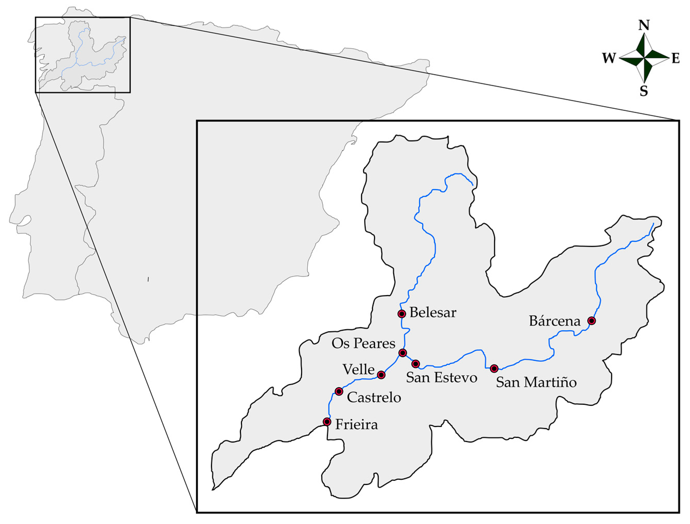
2.1. Area of Study

In this study, eight reservoirs belonging to the Miño-Sil basin (northwest of the Iberian Peninsula) were used as the study area. Of all these reservoirs, seven are located in Galicia (Belesar (Lugo), Frieira (Pontevedra–Ourense), San Estevo (Lugo–Ourense), Castrelo, Os Peares, San Martiño and Velle (Ourense)), while one is in Castilla–León (Bárcena (León)) (Figure 1).

The Spanish part of the Miño-Sil hydrographic demarcation has an area of 17,581.98 km² (89.73% of the total surface). It is also estimated to contain a population of up to 795,407 inhabitants and a density of around 45 inhabitants/km² [57]. Nowadays, the Sil and the Miño rivers constitute one of the electricity-producing regions in Spain [58]. Of the eight reservoirs analyzed, Belesar is the largest, with a total capacity of 654.66 hm³, while San Martiño reservoir is the smallest, with a total capacity of 9.60 hm³. All reservoirs have hydrologic uses. The Bárcena reservoir has, in addition to hydrological uses, water supply and irrigation uses [59].

2.2. Data Used

On request, 22 hydrological years on a daily scale were supplied by the Confederación Hidrográfica del Miño-Sil [60]. The time series data provided included the level of the reservoir (m.a.s.l.), the flow of contribution or entrance of the reservoir (m³/s), the output flow of the reservoir (m³/s) and the hm³ and the percentage (%) of volume of the reservoir between 1 January 2000 and 5 October 2022. The data used covers from 1 October 2000 to 30 September 2022, and the time series data used included the inflow and output flow of the reservoir (m³/s) and the volume of the reservoir (%) as input variables and as the output variable, the output flow of reservoir one day ahead (m³/s). The choice of these three variables is because they are easily accessible through the Miño-Sil Hydrographic Confederation, and in a past research, they have provided good results [1].

For the development of the different models, the database was divided into four groups: the training group (T) (between 1 October 2000 and 30 September 2013); the validation group (between 1 October 2013 and 30 September 2016); and two test groups Z₁ subset (between 1 October 2016 and 30 September 2019) and Z₂ subset (between 1 October 2019 and 30 September 2022).

2.3. Machine Learning Models

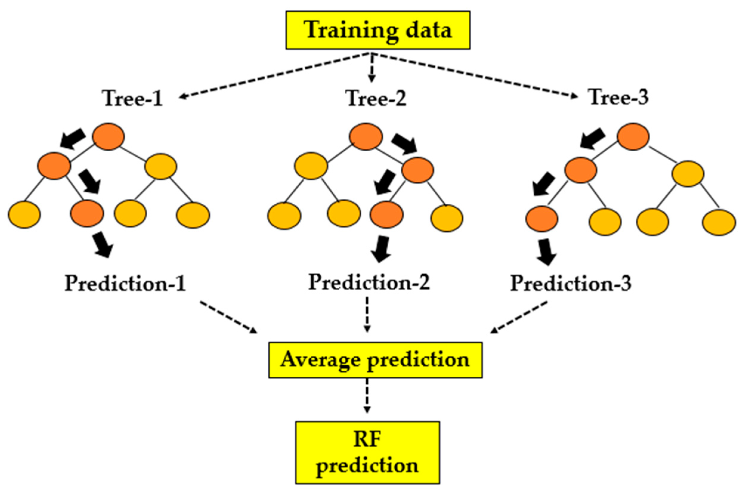
2.3.1. Random Forest

Random Forest (RF, Figure 2) is an ensemble supervised ML approach, introduced firstly by Breiman (2001) [61], based on a combination of decision trees [62], and is an adequate procedure to capture non-linear dependencies [63]. In fact, it is an improvement on the decision tree algorithm [64] since RF uses two elements of randomness to generate uncorrelated decision trees that become part of the forest, increasing the diversity among the trees [63]. This technique can use classification or regression trees to solve both kinds of problems [63,65].

An RF algorithm is trained using the “bagging method”, introduced by Breiman (1996) [66], in which a data subset is estimated from the original dataset chosen randomly with replacement, which helps to reduce the tree variance [67]. The bagging method includes two important steps: bootstrapping and aggregation [64]. Regarding bootstrapping, it is a technique that aims to produce new random training sets from the original training set, both of similar size, by a random selection with replacement [64]. According to Das et al. (2023) [64], this step is used to decrease the sensitivity of the model to the training data and decrease the probability of the model to overfit. Afterward, a random subset of features is selected from the total set of features to build decision trees and serves to decrease the correlation between trees [64].

Regarding a decision tree, depending on the function of the input attribute values, each internal node splits into two or more sub-spaces [68]. This process continues until the node cannot split further, converting to a terminal or leaf node [62].

In the regression tasks, the output prediction assigned to the sample is determined by averaging the forecasting of each individual decision tree [64,69]. On the other hand, in classification tasks, the majority vote is the criterion used to estimate the output prediction [64,69].

In this work, RF models were developed using different hyperparameter combinations: number of trees; criterion; maximal depth; and applying pre-prunning. In this study, the RF algorithm was implemented by studying the number of trees between 1 and 100 (99 steps, linear scale), the maximal depth between 1 and 100 (99 steps, linear scale), and applying pre-pruning (true and false). In addition to the models developed using the real scale of the involved variables (RF models), some variations of the model were carried out using range transformation between −1 and 1. This normalization was applied to the input variables (RF_N) and the input and the output variables and de-normalizing the results (RF_{N_D}) to compare the models with each other. The normalization process was carried out with the training data and was then applied to the validation and querying phases.

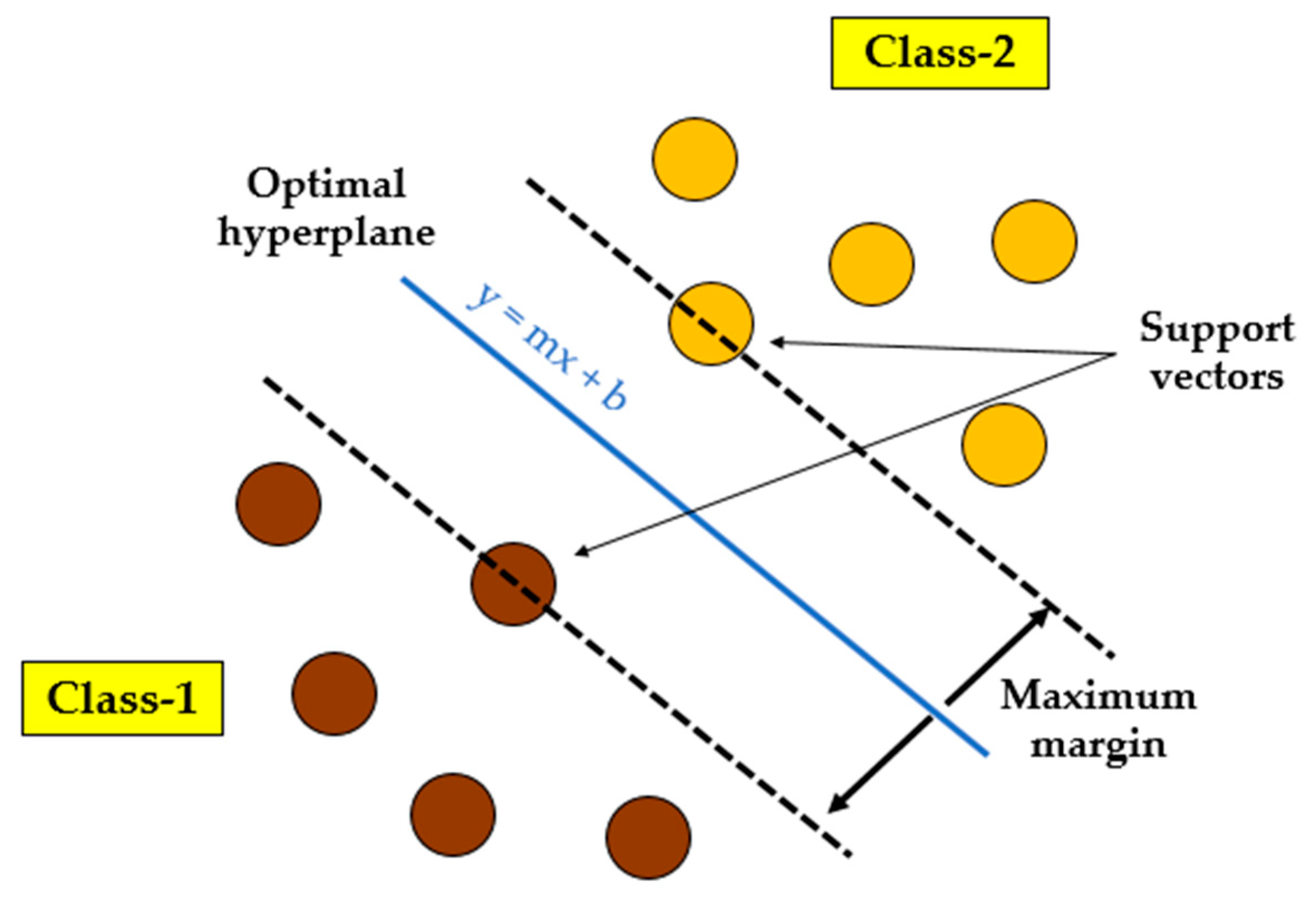
2.3.2. Support Vector Machine

According to Antonanzas-Torres et al. (2015) [70], the Support Vector Machine (SVM) is another supervised learning machine algorithm that was first introduced by Cortes and Vapnik (1995) [71] for classification problems, and later a regression variant was added by Vapnik (1995) [72] to solve regression problems. The SVM algorithm is a binary classifier in that its main role is to find an optimal hyperplane that presents a maximum margin between the feature vectors of all data in two categories [73] (Figure 3).

This algorithm is used to resolve both linear and nonlinear problems, the latter through the use of the kernel function transformation [75]. The kernel function is used to project input data from a lower dimensional space into a higher dimensional feature space [76,77].

In this work, SVM models were developed using different hyperparameter combinations; svm type, C and gamma. The Hsu, Chang and Lin (2003) [78] guide was followed to study the performance of the gamma and C parameters. In this research, SVM was studied using svm types (epsilon-SVR and nu-SVR), C values (between 0.03125 and 32,768 utilising 20 steps with a linear or logarithm scale), and gamma values (between 2⁻¹⁵ and 8 utilising 18 steps with a linear- or logarithm-scale subscript L-). In addition, in this case, different models were developed using range transformation between −1 and 1 to the input variables (SVM_N) and normalizing the input and output variables, then de-normalizing the results (SVM_ND) to compare the models with each other. The normalization process was carried out with the training data and was then applied to the validation and querying phases.

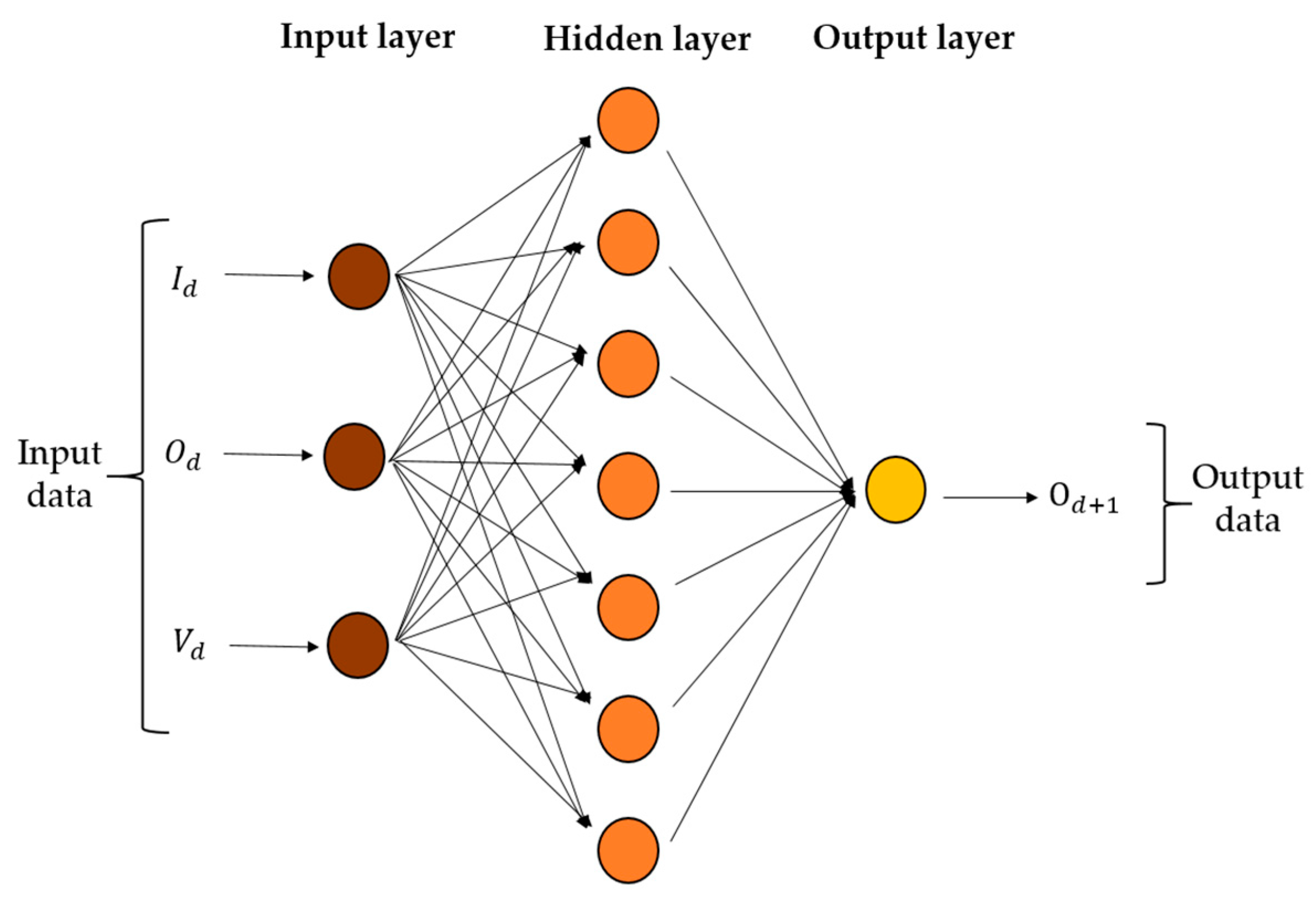
2.3.3. Artificial Neural Network

An artificial neural network (ANN) is an intelligent computational system that mimics biological neural networks [79,80]. In fact, this system is considered a possible tool to model complex relations between the input and output variables or to identify patterns [79]. An ANN is usually used in problems in which output variables are determined from huge input variables [81,82].

The architectures of ANNs are very variable and can be classified according to (i) the number of layers into single-layer and multiplayer networks or (ii) the direction of information flow and processing into feed-forward, recurrent and self-organizing networks [83]. According to Teke et al. (2023) [79], a multilayer feed-forward neural network is the most widely used ANN architecture. In this architecture class, ANN includes three layers known as input, hidden (one or more) and output layers [83,84] (Figure 4).

The information is moved between neurons in a direction from the input layers to the output layers [81,85]. Each neuron is connected to each next layer neuron through links [81], but this type of link is not established between neurons in the same layer [85]. Each neuron link can be understood as a connection strength, called weight [85]. The general learning process in a neural network is as follows: The input data are received in the input layer; which includes as many neurons as input variables [81]. The second layer, which receives the information from the input layer, is the most important of the ANN [81] and is responsible for calculating the weight and bias of the variable through an activation function [86]. Finally, the information from the previous layer is moved to the output layer, in which the output results are calculated with an error estimation [81,86].

According to Dragović (2022) [87], the training consists of synaptic weights modification between the different neurons in order to reduce the error between the real and the predicted value for the training cases. In fact, the modification of the synaptic weights is carried out by means of learning algorithms [87]. There are different training algorithms, but, according to Dragović (2022) [87], the backpropagation (BP) algorithm is the most used [88,89].

In this study, ANN models were developed using different topologies, training cycles and decay. The optimum values for each parameter were determined using the trial-and-error approach. The ANN was studied using different topologies (varying the hidden neurons number in the range of 2n + 1, n corresponding to the number of input variables), training cycles (1 to 131,072 utilising 17 steps, linear or logarithm scale) and decay (true or false). In addition, in this case, different models were developed using range transformation between −1 and 1 to the input variables and the output variables, then de-normalizing the results (ANN_ND) to compare the models with each other. The normalization process was carried out with the training data and was then applied to the other phases.

2.4. Metrics

To measure the model’s accuracy, different statistical parameters were used. These, according to Morasi et al. (2007) [90], can be divided into three groups: (i) standard regression statistics (Pearson’s coefficient of correlation, r); (ii) error index (root mean squared error (RMSE), RMSE-observations standard deviation ratio (RSR), and the percent bias (PBIAS)); and (iii) dimensionless statistics (Nash–Sutcliffe efficiency (NSE) [91]).

Pearson’s coefficient of correlation evaluates the collinearity between the predictions and the real value with a range of −1 and 1 [90]. RMSE—Equation (1)—and RSR—Equation (2)—quantify the variation in predicted values with respect to the real values in the data units used [90], and PBIAS—Equation (3)—measures the average tendency of the predicted data to be lower or higher than its observed counterparts [90,92]. Finally, the Nash–Sutcliffe efficiency—Equation (4)—provides information on the fit of the data to the 1:1 line [90]. In these equations, Y_obs are real values, Y_pred are values predicted by the model, Y_mean is the mean of all real data, and n is the total number of real data.

To select the best model among all the models developed for the same approach type, the lowest RMSE value for the validation phase was used.

$$\mathrm{RMSE}=\sqrt{\frac{1}{n}{\displaystyle \sum }_{i=1}^n{({\mathrm{Y}}_{\mathrm{obs}}-{\mathrm{Y}}_{\mathrm{pred}})}^2}$$

(1)

$$\mathrm{RSR} = \frac{\sqrt{{{\displaystyle \sum }}_{i=1}^N{\left({\mathrm{Y}}_{\mathrm{obs}}-{\mathrm{Y}}_{\mathrm{pred}}\right)}^2}}{\sqrt{{{\displaystyle \sum }}_{i=1}^N{\left({\mathrm{Y}}_{\mathrm{obs}}-{\mathrm{Y}}_{\mathrm{mean}}\right)}^2}}$$

(2)

$$\mathrm{PBIAS}=\frac{{{\displaystyle \sum }}_{i=1}^N\left({\mathrm{Y}}_{\mathrm{obs}}-{\mathrm{Y}}_{\mathrm{pred}}\right)}{{{\displaystyle \sum }}_{i=1}^N{\mathrm{Y}}_{\mathrm{obs}}}\times 100$$

(3)

$$\mathrm{NSE}=1-\frac{{{\displaystyle \sum }}_{i=1}^N{\left({\mathrm{Y}}_{\mathrm{obs}}-{\mathrm{Y}}_{\mathrm{pred}}\right)}^2}{{{\displaystyle \sum }}_{i=1}^N{\left({\mathrm{Y}}_{\mathrm{obs}}-{\mathrm{Y}}_{\mathrm{mean}}\right)}^2}$$

(4)

3. Results and Discussion

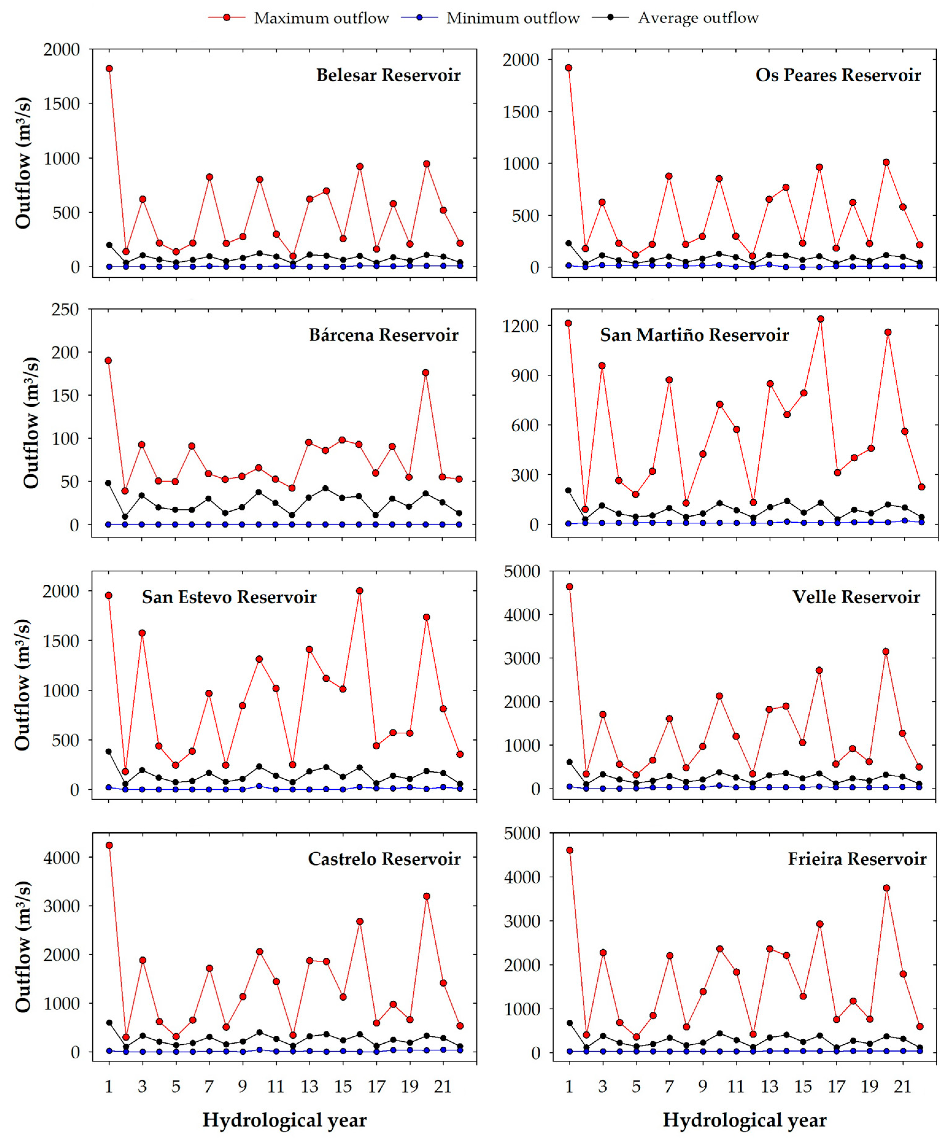
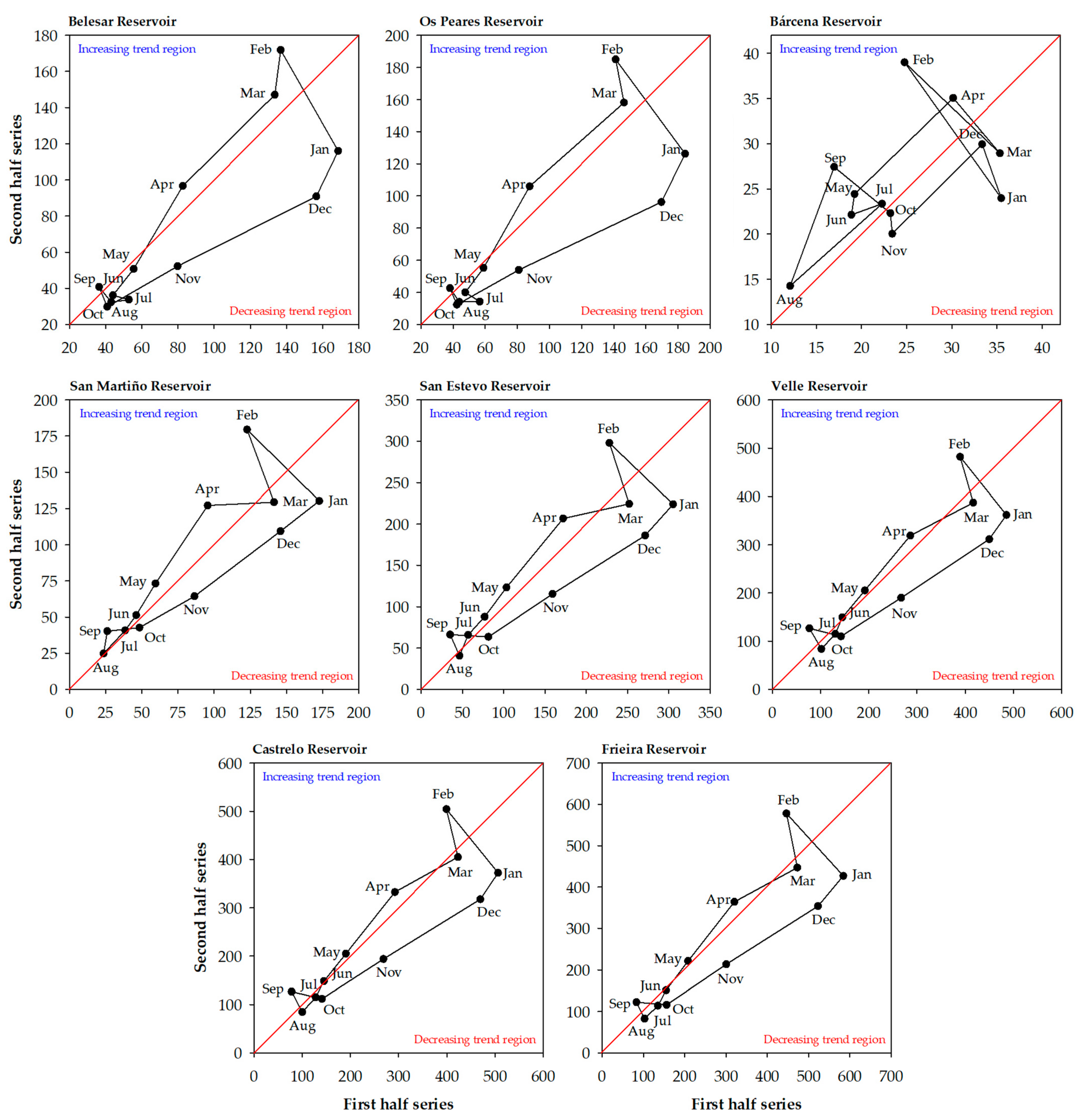
3.1. Data Analysis

With the entire time series (2000–2022), the maximum, minimum and average values for the output variables of each reservoir were calculated. The behavior of the maximum flow presented a saw profile, indicating the great variability between the years studied Figure 5. Large differences were observed in terms of the maximum output volume for, for example, the Velle reservoir, where in December 2000 an output flow of 4637 m³/s was recorded compared to other maximum values of only 313 m³/s. The average output flow presented a more stable behavior, notable for the absence of those pronounced saw teeth, than the maximum output flow presented. In fact, looking again at the Velle reservoir, it can be seen that the average flow varied from a maximum of 608 m³/s to more moderate flows around 100–180 m³/s.

Next, a brief study of innovative polygon trend analysis (IPTA) was carried out aimed at identifying the behavior of the outflow during the entire time series studied. For this, the twenty-two hydrological years were divided into two equal groups of eleven years, on the one hand, the first eleven years (2000–2011), and on the other hand, the last eleven hydrological years (2011–2022). Figure 6 presents, for each station, the IPTA method results, which were applied to the average data.

None of the reservoirs analyzed showed a regular polygon. Although, at first, it seems that the upper part of the polygon was regular, the lower part was highly unstable, with many crossings between the monthly lines. In general, a large change in the output flow (length of the lines) was observed for the autumn, winter and spring months, while for the summer months, the change was very small (short lines). It can also be seen that, for the Belesar and Os Peares reservoirs, the polygon was wider than in the rest of the reservoirs. This means that there was a greater outflow heterogeneous temporal variation compared to the other reservoirs. Finally, and based on the different graphs in Figure 6, it can be stated that in all the reservoirs there is a clear decrease in the outflow flow because most of the months are below the 1:1 line.

3.2. Machine Learning Models Developed

Numerous models were developed for each ML algorithm (RF, SVM and ANN). Afterward, the better models for each RF, SVM and ANN algorithms carried out in each reservoir were selected using the criterion of the lowest value of RMSE in the validation phase.

The

Table 1. Better models for each RF, SVM and ANN algorithms for each reservoir. RMSE is the root mean squared error (m³/s) and r is the Pearson’s correlation coefficient for the real and the predicted values. Models in bold correspond to the best model. Adapted from Sobrido Pouso (2023) [54].

	T		V		Z		Z2
Model	RMSE	r	RMSE	r	RMSE	r	RMSE	r
Belesar
RFND	28.6	0.962	31.4	0.952	27.5	0.908	34.6	0.937
SVMN	31.9	0.952	31.0	0.953	24.8	0.926	33.5	0.942
ANNN-L	32.8	0.950	30.2	0.955	24.1	0.929	32.1	0.947
Os Peares
RFN	30.8	0.965	36.0	0.944	27.2	0.924	39.5	0.927
SVMND	37.8	0.947	35.9	0.944	26.6	0.927	36.0	0.940
ANN	44.1	0.930	36.5	0.942	27.1	0.924	36.1	0.940
Bárcena
RFND	7.2	0.948	9.0	0.930	8.1	0.918	9.7	0.917
SVMN-L	7.7	0.941	8.9	0.931	7.7	0.926	9.7	0.916
ANNND-L	7.7	0.940	8.9	0.933	7.9	0.922	9.4	0.920
San Martiño
RF	34.3	0.943	44.6	0.939	18.6	0.942	37.8	0.936
SVML	34.9	0.943	43.5	0.946	17.5	0.950	44.6	0.915
ANNND	34.9	0.941	44.6	0.939	17.9	0.947	32.5	0.951
San Estevo
RFND	47.3	0.967	70.5	0.937	30.9	0.937	47.2	0.957
SVMND-L	59.9	0.948	69.6	0.939	32.5	0.935	49.1	0.954
ANNND	58.5	0.950	68.1	0.941	31.3	0.937	48.0	0.956
Velle
RFND	71.0	0.970	95.5	0.941	50.1	0.937	88.2	0.946
SVMND-L	101.9	0.937	92.4	0.945	51.0	0.935	79.7	0.959
ANNND	100.2	0.938	91.7	0.946	47.8	0.943	78.4	0.958
Castrelo
RF	69.6	0.972	94.9	0.949	59.5	0.927	94.0	0.946
SVMN-L	91.7	0.951	95.4	0.950	51.0	0.944	88.8	0.955
ANNND	87.6	0.954	94.1	0.949	50.5	0.946	171.1	0.876
Frieira
RFND	98.7	0.956	122.6	0.938	68.3	0.930	104.9	0.949
SVMND	104.7	0.951	118.5	0.944	65.6	0.939	111.7	0.949
ANNND	105.5	0.950	118.8	0.942	62.7	0.941	118.4	0.936

Note: ANN: Artificial neural network; ANN_N-L: Artificial neural network normalize in logarithm scale; ANN_ND: Artificial neural network normalize de-normalize; ANN_ND-L: Artificial neural network normalize de-normalize in logarithm scale; RF: Random Forest; RF_N: Random Forest normalize; RF_ND: Random Forest normalize de-normalize; SVM_L: Support Vector Machine in logarithm scale; SVM_N: Support Vector Machine normalize; SVM_N-L: Support Vector Machine normalize in logarithm scale; SVM_ND: Support Vector Machine normalize de-normalize; SVM_ND-L: Support Vector Machine normalize de-normalize in logarithm scale.

shows the statistical parameters used to assess the performance of models in predicting outflow from reservoirs one day ahead.

Within the different Random Forest models developed (RF, RF_N and RF_ND), it can be observed that RF_ND was the best Random Forest model for most of the reservoirs (except for Os Peares, San Martiño and Castrelo) with RMSE values in validation phase varying between 9.0 m³/s for Bárcena and 122.6 m³/s in the case of Frieira. Regarding the developed SVM algorithms (SVM, SVM_L, SVM_N, SVM_N-L, SVM_ND and SVM_ND-L) the best model depended on the analyzed reservoir, since in each one of the eight reservoirs, different variants of the SVM algorithm showed the lowest values of RMSE in the validation phase. In this sense, the lowest RMSE value (8.9 m³/s) was shown derived by the SVM_N-L algorithm (Bárcena). On the contrary, the SVM_ND algorithm (Frieira) showed the highest RMSE value (118.5 m³/s). Finally, in the case of the ANN models developed (ANN, ANN_L, ANN_N, ANN_N-L, ANN_ND and ANN_ND-L), the ANN_ND algorithm was the best model in most of the reservoirs analyzed (except Belesar, Os Peares and Bárcena). The RMSE values in the validation phase varyied between 8.9 m³/s for Bárcena and 118.8 m³/s for Frieira. According to all results mentioned above, it can be concluded that there is no single model that is capable of finding the best results for all reservoirs. That is, each reservoir has their own best role models.

The best model among the three selected models for each reservoir could also be chosen based on the RMSE value in the validation phase. In this sense, it can be seen that the best models were obtained using the ANN algorithm in five reservoirs (Belesar, Bárcena, San Estevo, Velle and Castrelo), being that the ANN_ND model was the one that showed the best results on three occasions. According to these results, the ANN algorithm seems to be a more suitable technique in this type of task, probably due to the non-linear nature of the event. The Support Vector Machine model was the best model in three of the analyzed reservoirs, being that the SVM_ND was the best model for Os Peares and Frieira and SVM_L was the best model for the San Martiño reservoir. No RF model showed better results for any reservoir, which suggests that this algorithm is not suitable for this type of task.

Detailing the results of the best model for each reservoir, different behaviors can be observed between the training (T), validation (V), test (Z) and test-2 (Z₂) phases.

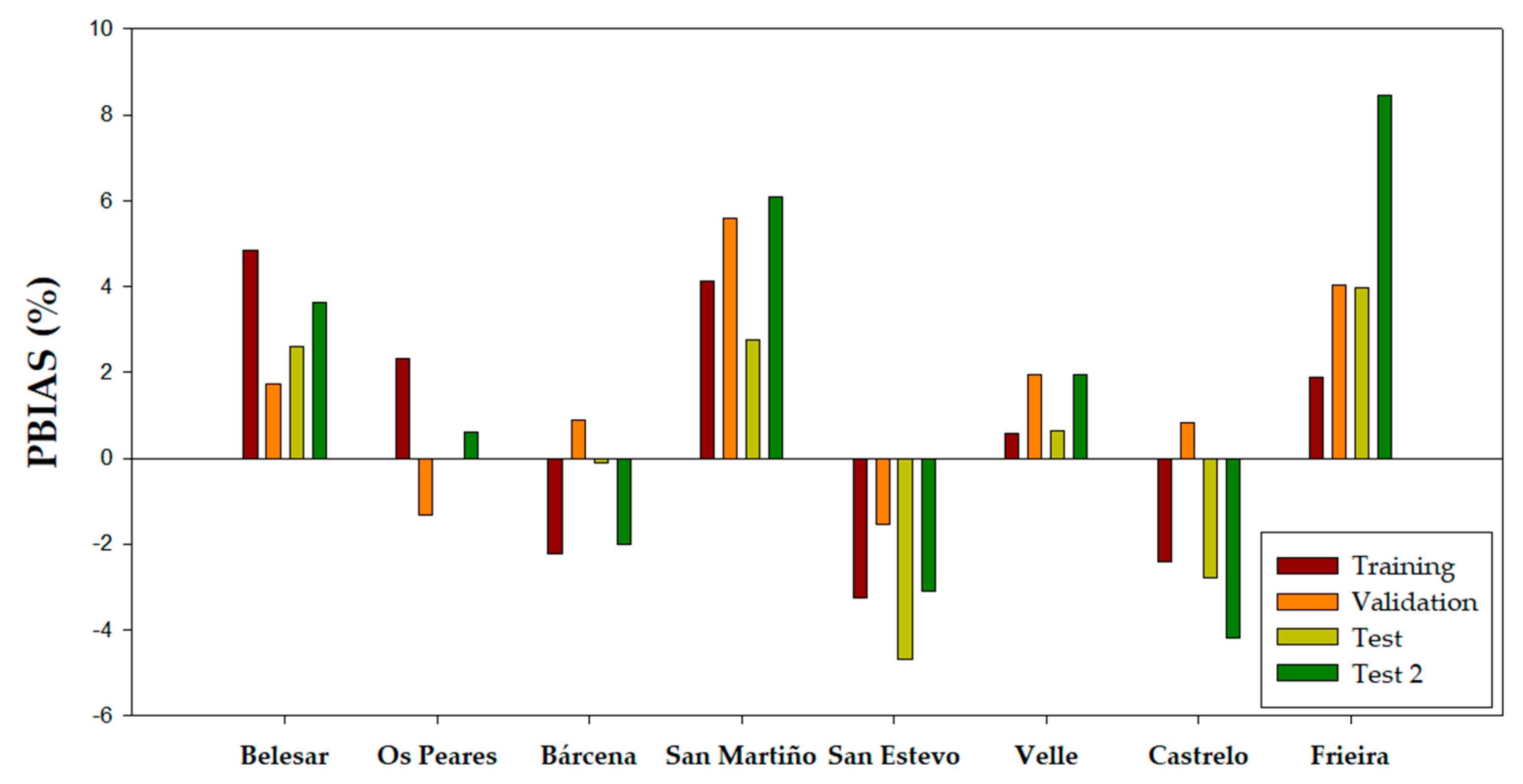
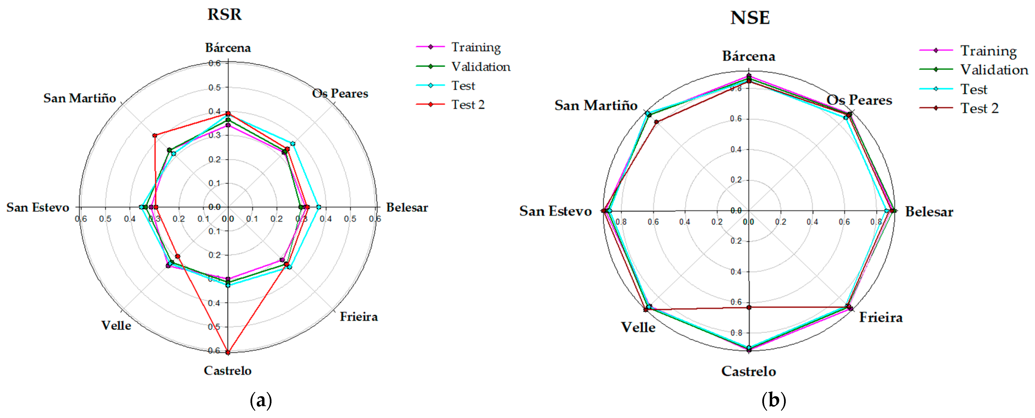
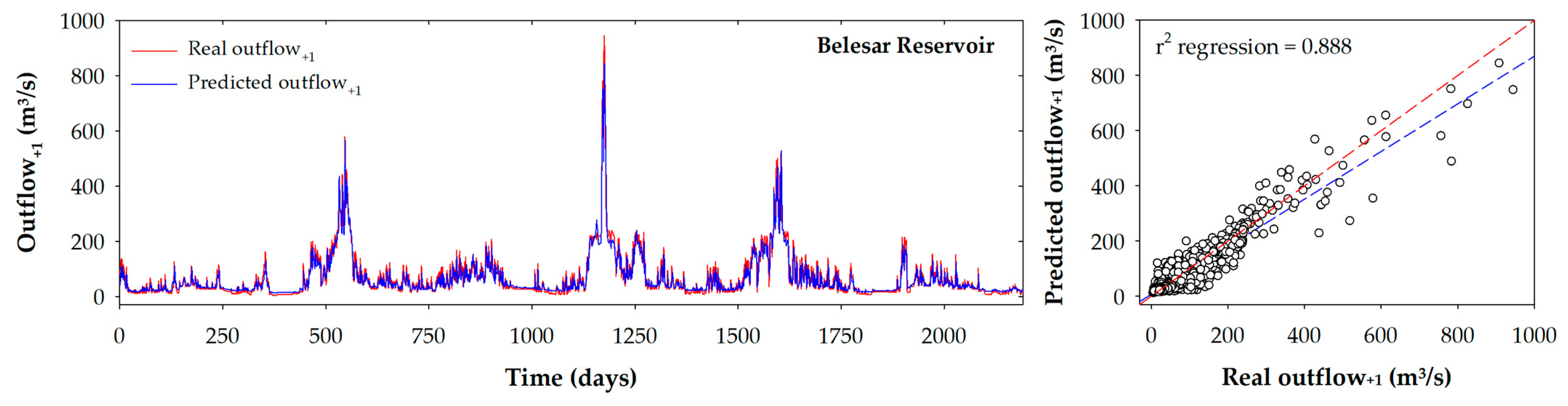
• ANN_N-L was the best model for the Belesar reservoir. This model showed good fit in relation to RMSE and r value in the validation phase (RMSE = 30.2 m³/s and r = 0.955). The other two selected models presented RMSE values close to the ANN_N-L model (31.4 m³/s and 31.0 m³/s for the RF_ND and the SVM_N model, respectively). ANN_N-L showed similar statistics in the training phase, with a slightly higher RMSE value of 32.8 m³/s. In the test phase, RMSE was 24.1 m³/s. However, the RMSE value increased to 32.1 m³/s in the test-2 phase. This increase in the test-2 phase was not unique for this model but was also observed in the rest of the models This behavior can be caused by the outflow range to test phase being less than the range in test-2 phase.
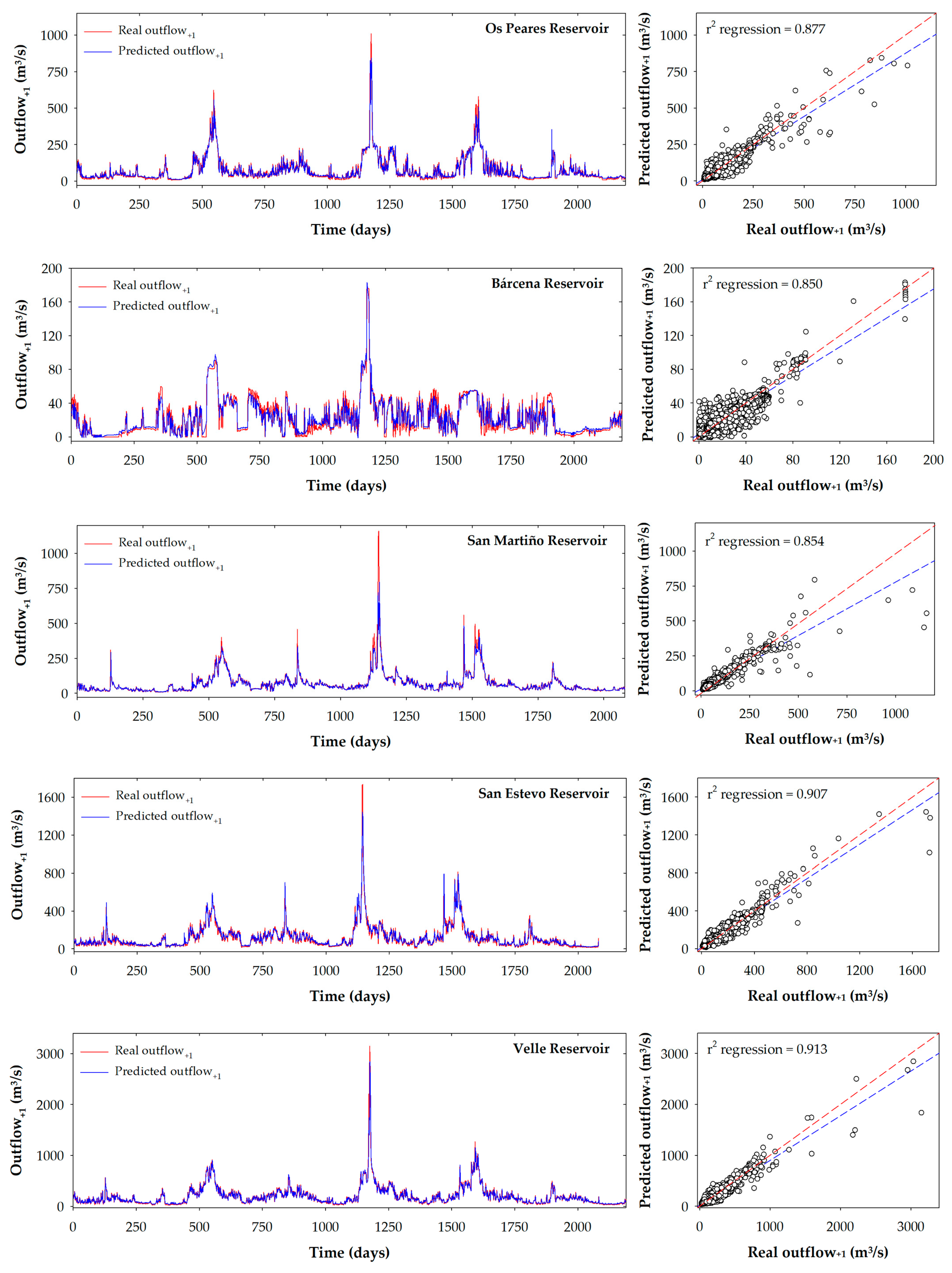
• Regarding the Os Peares reservoir, SVM_ND was the model that provided the best statistics in relation to the RMSE value in the validation phase (RMSE = 35.9 m³/). The good adjustments provided by this model during the validation phase were very close to the second best model, the RF_N (36.0 m³/s). The model SVM_ND showed a similar behavior in the training phase with a slightly higher RMSE value of 37.8 m³/s. The RMSE value in the test phase was 26.6 m³/s. However, an increase in the value of the root mean squared error in the test-2 phase (36.0 m³/s) can be observed, as happened with the best model of the previous reservoir.
• Regarding Bárcena, the three models selected for this reservoir presented very similar RMSE adjustments for the validation phase with values between 8.9 and 9.0 m³/s. The ANN_ND-L model showed the lowest RMSE value (8.9 m³/s -8.86-) with an r of 0.933. This model presented similar statistics in the training phase, with a slightly lower RMSE value of 7.7 m³/s. The behavior shown by this model in the test phase was similar to the training and validation phase (RMSE = 7.9 m³/s), having an increase in its value for the test-2 phase (9.4 m³/s).
• In the case of San Martiño, all the selected models were in a very close RMSE value range for the validation phase, with values between 43.5 and 44.6 m³/s, with the SVM_L model being the best with an RMSE and r of 43.5 m³/s and 0.946, respectively. This model presented different statistics in the training and test phase, with an RMSE value of 34.9 m³/s and 17.5 m³/s, respectively. However, in the test-2 phase, the SVM_L model was similar to the validation phase, with a slightly higher RMSE value (44.6 m³/s).
• ANN_ND was the best model for the San Estevo reservoir, in which the RMSE value in the validation phase was 68.1 m³/s and r of 0.941. The other two selected models presented an RMSE value close to that shown by the ANN_ND model (70.5 and 69.6 m³/s for the RF_ND and the SVM_ND-L, respectively). The ANN_ND model presented a different behavior in the training and test phase with RMSE values of 58.5 m³/s and 31.3 m³/s, respectively. However, in the test-2 phase, the RMSE increased to 48.0 m³/s.
• For the Velle reservoir, the different selected models presented highly differentiated RMSE values (between 91.7 and 95.5 m³/s), which was not the case in the rest of the reservoirs (except Frieira). In this case, the best model was the ANN_ND model, showing the lowest RMSE (91.7 m³/s) and highest r value (0.946) in the validation phase. In the training phase, it presented a higher RMSE value of 100.2 m³/s and the behavior observed for the test and test-2 phases (47.8 and 78.4 m³/s) followed the same pattern as the rest of the models.
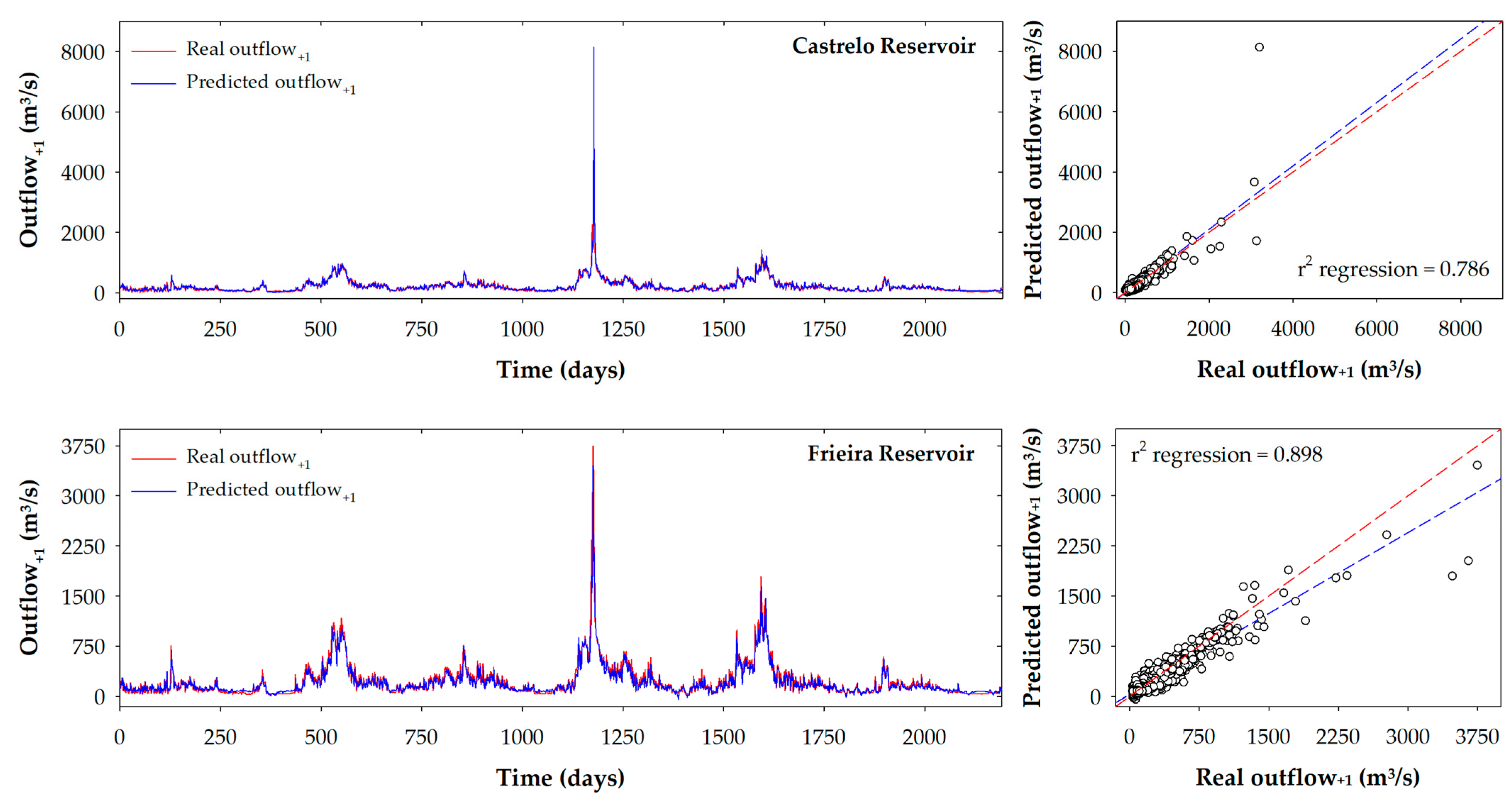
• The ANN_ND model was the best-selected model for the Castrelo reservoir, presenting the best statistics in the validation phase (RMSE = 94.1 m³/s). The other two models presented very similar values (94.9 m³/s for the RF model and 95.4 m³/s for the SMN_N-L model). The ANN_ND model behavior in the training phase presented an RMSE value of 87.6 m³/s. Although for the test phase, the model presented good results (50.5 m³/s) for test-2 phase, the ANN_ND model presented a very high RMSE value (171.1 m³/s) compared to the rest of the phases.
• Finally, the best model of the Frieira reservoir (SVM_ND) showed an RMSE value for the validation phase of 118.5 m³/s and a higher r value (0.944). The rest of the selected models presented RMSE values of 122.6 m³/s (RF_ND) and 118.8 m³/s (ANN_ND) for this phase. The model presented different statistics for training and test phases, in which RMSE values were 104.7 m³/s and 65.6 m³/s, respectively. In the test-2 phase, the RMSE value increased to 111.7 m³/s.

There are other statistical metrics, such as PBIAS, RSR and NSE, that also were evaluated to better understand the performance of the models. Regarding PBIAS (Figure 7), a value closest to 0 leads to lower error predicted data with relation to observed data, indicating best fit [90,92].

The models for Belesar, San Martiño, Velle and Frieira reservoirs, showed positive PBIAS values in all phases (T, V, Z and Z₂), indicating model underestimation bias. On the other hand, the model for San Estevo showed negative PBIAS values in all phases, indicating model overestimation bias. The models for the remaining reservoirs (Os Peares, Bárcena and Castrelo, respectively) showed both positive and negative PBIAS values depending on the phase. In the Os Peares and Bárcena models, showed PBIAS values closest to 0 (PBIAS = −0.01% and −0.10%, respectively) in the test phase, indicating an accurate prediction. The highest negative PBIAS value, in the test phase, was −4.69% obtained by San Estevo model. On the other hand, the maximum PBIAS value in the test-2 phase was obtained by the Frieira model (8.45%). Finally, the San Martiño and Frieira models, underestimated the observed data (PBIAS values between 2.75% and 6.11%, and between 1.90% and 8.45%, respectively), while San Estevo and Castrelo models showed that the predicted data overestimated the observed data (PBIAS values between −1.54% and −4.69% for San Estevo, and between 0.83% and −4.17% for Castrelo, although, in this last case, a slight underestimation was also observed in the validation phase).

In view of the results provided by the best-selected models it can be concluded that for PBIAS values, the mean tendency of the simulated values compared to their observed counterparts are not far from the 0 value (considered optimal).

The RSR values for each best reservoir model are shown in Figure 8. As can be observed, the best model of each reservoir showed RSR values similar in training, validation and test phases. The range was from 0.297 (validation phase, Belesar) to 0.386 (Z phase, Bárcena). On the contrary, a larger difference in RSR values can be observed in the test-2 phase. The range varied between 0.291 (Velle) and 0.608 (Castrelo) and San Martiño and Castrelo showed the highest RSR values (0.423 and 0.608, respectively). The presence of data predicted by these models that was far from the observed data leads to a worse fit and consequently an increase in the RSR value, indicating an inaccurate simulation of the model. The optimum RSR value is 0, indicating a good simulation of the model [90]. Considering this, the models for San Estevo and Velle, showed the most accurate simulations, since the RSR values were below 0.355 in all phases, highlighting the lowest RSR values in the test-2 phase (0.294 and 0.291, respectively).

Figure 8 also shows the NSE values of better models for each reservoir. As can be observed, the best model of each reservoir presented NSE values similar in training, validation and test phases. The range varied between 0.851 (test phase, Bárcena) and 0.912 (validation phase, Belesar). Considering these results, the variation between observed and predicted data by the best model of each reservoir was not high, being similar in, practically, all phases. However, important differences can be observed in the test-2 phase, since the range was from 0.631 to 0.916. Taking into account that the optimal value of NSE is 1 [90], and the farther the NSE value is from 1, the greater the difference between the observed and predicted data by the model, The Castrelo model showed the lowest NSE value in the test-2 phase (0.631), indicating that the simulations and observations were not similar. In fact, ANN_ND models (San Estevo and Velle) showed the best fit between observed and predicted data in all phases (NSE equal to or greater than 0.880). These models showed the lowest dispersion between simulated and real data.

Next, to further illustrate the behavior of the models, an analysis of the predicted and observed outflow time series for the test phases (Z and Z₂) for each reservoir has been developed (Figure 9). The test phase (Z) (October 2016 to September 2019) corresponded to 1075 days (San Martiño and San Estevo), and 1095 days (rest reservoirs). The test-2 phase (Z₂) (October 2019 to September 2022) contained 1005 days (San Martiño), 1007 days (San Estevo) and 1096 days (rest of reservoirs). In this sense, the total phase (ZZ₂) corresponded 2080 days (San Martiño), 2082 days (San Estevo) and 2191 days (rest of reservoirs). The red line corresponds to the predicted outflow and the back line to the observed outflow. Generally, the range of outflow was high in all reservoirs, except for Bárcena, in which the range was from 0 to 176 m³/s.

Figure 9 shows that the outflow range for Z₂ was higher than for Z in all reservoirs because of there was an important high peak of outflow that corresponded to a period of high rainfall which occurred during the month of December 2019 and led to a considerable increase in river flows. In this case, the models were not capable of fitting correctly. This may be the reason that the RMSE values in the test-2 phase (Z₂) were worse than in the test phase (Z) in all models (Table 1). The difference in RMSE values between Z and Z₂ phases was important in all models of each reservoir (20.2% in Bárcena, 33.3% in Belesar, 35.5% in Os Peares, 53.5% in San Estevo, 64.1% in Velle and 70.3% in Frieira), highlighting the difference shown by the Castrelo model and San Martiño model, 238.6% and 154.8%, respectively. In fact, the Castrelo model predicted an outflow of 8138.8 m³/s vs. the real value of 3197.2 m³/s and the San Martiño model predicted a value of 453.5 m³/s vs. the real value of 1145.8 m³/s. Furthermore, in the rest of reservoirs, the models were also not capable of predicting the outflow with accuracy. For example, in the case of Frieira, Velle and San Estevo, the best model predicted 1798.2 m³/s, 1835.7 m³/s and 1012.9 m³/s, respectively, while the observed values were 3476.3 m³/s, 3148.8 m³/s and 1729.2 m³/s, respectively. Furthermore, for the peak observed in the Os Peares reservoir, the SVM_ND model predicted a flow of 524.6 m³/s for an actual flow of 846.4 m³/s. Finally, the Belesar model and Bárcena model predicted a value of 489.4 m³/s and 88.2 m³/s, respectively, vs. the real value of 783.4 m³/s and 38.8 m³/s, respectively. Therefore, all models of eight reservoirs poorly predicted high outflow situations.

On the other hand, the models also presented some difficulties in modeling outflows during intervals of very low outflows (dry events). Generally, the models, in these cases, predicted higher outflow values than those observed. The test and Test-2 periods presented some very dry years (especially, 2017, 2021 and 2022). For example, the Bárcena model showed problems in predicting events of very low flows (below 10 m³/s) which occurred from December 2016 to May 2017 (from 81 to 215 day) and between January and first half of August 2022 (from 1926 to 2145 day).

Our research group has recently collaborated on a similar study in which these three input variables were used to predict the outflow of a reservoir one day ahead [1]. In that study, the data range used was from 2000 to 2019, using the same data division used in this research (T, V and Z). However, in that study, ANN-based models (MLP, NARX and LSTM), among others, were mainly used. In general, the results obtained in relation to the values of r (above 0.93), NSE, RSR and PBIAS were quite good. When compared with this research, small variations could be observed in relation to the values of r, NSE and RSR, but, in general, were consistent with the data reported in this research.

According to these results, all models showed similar performances in normal conditions. That is, in normal period of flows, the model adequately predicted outflow. However, it is necessary to develop models that are also capable of correctly predicting situations of small and high flows, especially in floods and droughts situations, to facilitate management and defense against these adverse phenomena. The models presented in this research work correctly for intermediate flows; however, it would be desirable if they presented better adjustments for flood and drought periods, which can only be achieved with the gradual increase in the time series and the appearance of these phenomena. It is necessary to emphasize that the models developed in this work were implemented with only three input variables. These variables are easy to obtain and allow a correct prediction. To improve the model’s prediction, it would be necessary to incorporate other types of variables that could define the reservoir in depth, such as climatological, hydrological or orographic variables.

4. Conclusions

This work consisted of an evaluation of different machine learning models to determine the outflow one-day ahead using three input variables: inflow; outflow; and reservoir volume percent. RF, SVM and ANN models were developed for eight reservoirs belonging to the Miño-Sil Hydrographic Confederation. The best models were selected according to the criterion of lowest value of RMSE in the validation phase. In this sense, these models were ANN_N-L (Belesar), SVM_ND (Os Peares), ANN_ND-L (Bárcena), SVM_L (San Martiño), ANN_ND (San Estevo, Velle and Castrelo) and SVM_ND (Frieira). The ANN algorithm was the most suitable, since it was the best method in five reservoirs.

The models showed a good generalization performance with no significant signs of overfitting. However, a different behavior of the models was observed in the test-2 phase (Z₂). The general observations suggested that the analyzed ML models are suitable to predict outflow of reservoirs in normal conditions and, for this reason, these can be integrated into early warning or water resource management systems. However, the prediction of these models against small and high flows is not as good as it should be.

Although these models were developed using only three input variables, there are other variables that could influence outflows, such as (i) precipitation, (ii) humidity, or (iii) electricity demand, among others. It would also be interesting to develop models to predict outflow for a longer period (two, three, six days, etc.) and consider the possible effects that may exist on the variables selected in this research (or in future research) that are due to climate change. These variables (input and output) should not be included at random, but rather, different combinations of them should be studied. Although this would be the most appropriate way to proceed, it must be considered that this procedure would require a large quantity of time and computational cost (due to working with long time series) for which this study, or studies, should be carried out, trying to optimize, as far as possible, the use of available resources.

Likewise, it could study the influence that a different distribution of the database could have on the results of the models and the hyperparameters combination in different ranges, among others. It would be a good idea for the models to be updated with new data for reasonable periods of time.

Finally, it is necessary to highlight that as the models developed in this research have been implemented with general variables, and although they have had good results, this does not imply that these models will work in a similar way in reservoirs with different characteristics, such as orographic, climatic, or hydrological conditions. This warning should be considered when using models outside their scope of development since the inherent conditions of the reservoir have a significant impact on the input and output variables.

References

1. García-Feal, O.; González-Cao, J.; Fernández-Nóvoa, D.; Astray Dopazo, G.; Gómez-Gesteira, M. Comparison of Machine Learning Techniques for Reservoir Outflow Forecasting. Nat. Hazards Earth Syst. Sci. 2022, 22, 3859–3874. [Google Scholar] [CrossRef]
2. Baba, A.; Tsatsanifos, C.; el Gohary, F.; Palerm, J.; Khan, S.; Mahmoudian, S.; Ahmed, A.; Tayfur, G.; Dialynas, Y.; Angelakis, A. Developments in Water Dams and Water Harvesting Systems throughout History in Different Civilizations. Int. J. Hydrol. 2018, 2, 150–166. [Google Scholar] [CrossRef]
3. Marques, É.T.; Gunkel, G.; Sobral, M.C. Management of Tropical River Basins and Reservoirs under Water Stress: Experiences from Northeast Brazil. Environments 2019, 6, 62. [Google Scholar] [CrossRef]
4. Hao, S.; Wörman, A.; Riml, J.; Bottacin-Busolin, A. A Model for Assessing the Importance of Runoff Forecasts in Periodic Climate on Hydropower Production. Water 2023, 15, 1559. [Google Scholar] [CrossRef]
5. Gemechu, E.; Kumar, A. A Review of How Life Cycle Assessment Has Been Used to Assess the Environmental Impacts of Hydropower Energy. Renew. Sustain. Energy Rev. 2022, 167, 112684. [Google Scholar] [CrossRef]
6. International Energy Agency Electricity Information: Overview. Available online: https://www.iea.org/reports/electricity-information-overview (accessed on 25 January 2021).
7. Cernea, M.M. Social Impacts and Social Risks in Hydropower Programs: Preemptive Planning and Counter-Risk Measures; George Washington University: Bethesda, MD, USA, 2004. [Google Scholar]
8. Panagiotou, A.; Zogaris, S.; Dimitriou, E.; Mentzafou, A.; Tsihrintzis, V.A. Anthropogenic Barriers to Longitudinal River Connectivity in Greece: A Review. Ecohydrol. Hydrobiol. 2022, 22, 295–309. [Google Scholar] [CrossRef]
9. Grill, G.; Lehner, B.; Thieme, M.; Geenen, B.; Tickner, D.; Antonelli, F.; Babu, S.; Borrelli, P.; Cheng, L.; Crochetiere, H.; et al. Mapping the World’s Free-Flowing Rivers. Nature 2019, 569, 215–221. [Google Scholar] [CrossRef]
10. Jeuland, M.; Baker, J.; Bartlett, R.; Lacombe, G. The Costs of Uncoordinated Infrastructure Management in Multi-Reservoir River Basins. Environ. Res. Lett. 2014, 9, 105006. [Google Scholar] [CrossRef]
11. Marques, G.F.; Tilmant, A. The Economic Value of Coordination in Large-Scale Multireservoir Systems: The Parana River Case. Water Resour. Res. 2013, 49, 7546–7557. [Google Scholar] [CrossRef]
12. Quinn, J.D.; Reed, P.M.; Giuliani, M.; Castelletti, A. What Is Controlling Our Control Rules? Opening the Black Box of Multireservoir Operating Policies Using Time-Varying Sensitivity Analysis. Water Resour. Res. 2019, 55, 5962–5984. [Google Scholar] [CrossRef]
13. Rougé, C.; Reed, P.M.; Grogan, D.S.; Zuidema, S.; Prusevich, A.; Glidden, S.; Lamontagne, J.R.; Lammers, R.B. Coordination and Control—Limits in Standard Representations of Multi-Reservoir Operations in Hydrological Modeling. Hydrol. Earth Syst. Sci. 2021, 25, 1365–1388. [Google Scholar] [CrossRef]
14. Shen, J.; Cheng, C.; Zhang, X.; Zhou, B. Coordinated Operations of Multiple-Reservoir Cascaded Hydropower Plants with Cooperation Benefit Allocation. Energy 2018, 153, 509–518. [Google Scholar] [CrossRef]
15. Wei, N.; He, S.; Lu, K.; Xie, J.; Peng, Y. Multi-Stakeholder Coordinated Operation of Reservoir Considering Irrigation and Ecology. Water 2022, 14, 1970. [Google Scholar] [CrossRef]
16. Kundzewicz, Z.W.; Kanae, S.; Seneviratne, S.I.; Handmer, J.; Nicholls, N.; Peduzzi, P.; Mechler, R.; Bouwer, L.M.; Arnell, N.; Mach, K.; et al. Flood Risk and Climate Change: Global and Regional Perspectives. Hydrol. Sci. J. 2014, 59, 1–28. [Google Scholar] [CrossRef]
17. Hassan, Z.; Razali, N.H.M.; Kamarudzaman, A.N.; Salwa, M.Z.M.; Nordin, N.A.S. Preliminary Study on Flood Simulation Using the HEC-HMS Model for Muda River, Malaysia. IOP Conf. Ser. Earth Environ. Sci. 2023, 1135, 012021. [Google Scholar] [CrossRef]
18. Nakamura, I.; Llasat, M.C. Policy and Systems of Flood Risk Management: A Comparative Study between Japan and Spain. Nat. Hazards 2017, 87, 919–943. [Google Scholar] [CrossRef]
19. UNISDR Impact of Disasters since the 1992 Rio de Janeiro Earth Summit. Available online: https://www.unisdr.org/files/27162_infographic.pdf (accessed on 20 July 2023).
20. European Environment Agency. Climate Change, Impacts and Vulnerability in Europe 2016 an Indicator-Based Report; European Environment Agency: Copenhagen, Denmark, 2017. [Google Scholar]
21. Llasat, M.C.; Marcos, R.; Llasat-Botija, M.; Gilabert, J.; Turco, M.; Quintana-Seguí, P. Flash Flood Evolution in North-Western Mediterranean. Atmos. Res. 2014, 149, 230–243. [Google Scholar] [CrossRef]
22. Fischer, S.; Schumann, A.; Bühler, P. Timescale-Based Flood Typing to Estimate Temporal Changes in Flood Frequencies. Hydrol. Sci. J. 2019, 64, 1867–1892. [Google Scholar] [CrossRef]
23. Persiano, S.; Ferri, E.; Antolini, G.; Domeneghetti, A.; Pavan, V.; Castellarin, A. Changes in Seasonality and Magnitude of Sub-Daily Rainfall Extremes in Emilia-Romagna (Italy) and Potential Influence on Regional Rainfall Frequency Estimation. J. Hydrol. Reg. Stud. 2020, 32, 100751. [Google Scholar] [CrossRef]
24. Hirabayashi, Y.; Mahendran, R.; Koirala, S.; Konoshima, L.; Yamazaki, D.; Watanabe, S.; Kim, H.; Kanae, S. Global Flood Risk under Climate Change. Nat. Clim. Chang. 2013, 3, 816–821. [Google Scholar] [CrossRef]
25. Zhao, Y.; Weng, Z.; Chen, H.; Yang, J. Analysis of the Evolution of Drought, Flood, and Drought-Flood Abrupt Alternation Events under Climate Change Using the Daily SWAP Index. Water 2020, 12, 1969. [Google Scholar] [CrossRef]
26. Wasko, C. Floods Differ in a Warmer Future. Nat. Clim. Chang. 2022, 12, 1090–1091. [Google Scholar] [CrossRef]
27. Liu, C.; Guo, L.; Ye, L.; Zhang, S.; Zhao, Y.; Song, T. A Review of Advances in China’s Flash Flood Early-Warning System. Nat. Hazards 2018, 92, 619–634. [Google Scholar] [CrossRef]
28. Wasko, C.; Nathan, R.; Stein, L.; O’Shea, D. Evidence of Shorter More Extreme Rainfalls and Increased Flood Variability under Climate Change. J. Hydrol. 2021, 603, 126994. [Google Scholar] [CrossRef]
29. Berghuijs, W.R.; Aalbers, E.E.; Larsen, J.R.; Trancoso, R.; Woods, R.A. Recent Changes in Extreme Floods across Multiple Continents. Environ. Res. Lett. 2017, 12, 114035. [Google Scholar] [CrossRef]
30. Westra, S.; Fowler, H.J.; Evans, J.P.; Alexander, L.V.; Berg, P.; Johnson, F.; Kendon, E.J.; Lenderink, G.; Roberts, N.M. Future Changes to the Intensity and Frequency of Short-Duration Extreme Rainfall. Rev. Geophys. 2014, 52, 522–555. [Google Scholar] [CrossRef]
31. Min, S.-K.; Zhang, X.; Zwiers, F.W.; Hegerl, G.C. Human Contribution to More-Intense Precipitation Extremes. Nature 2011, 470, 378–381. [Google Scholar] [CrossRef]
32. Donat, M.G.; Lowry, A.L.; Alexander, L.V.; O’Gorman, P.A.; Maher, N. More Extreme Precipitation in the World’s Dry and Wet Regions. Nat. Clim. Chang. 2016, 6, 508–513. [Google Scholar] [CrossRef]
33. Fischer, E.M.; Beyerle, U.; Knutti, R. Robust Spatially Aggregated Projections of Climate Extremes. Nat. Clim. Chang. 2013, 3, 1033–1038. [Google Scholar] [CrossRef]
34. De la Paix, M.J.; Lanhai, L.; Xi, C.; Ahmed, S.; Varenyam, A. Soil Degradation and Altered Flood Risk as a Consequence of Deforestation. L. Degrad. Dev. 2013, 24, 478–485. [Google Scholar] [CrossRef]
35. Peptenatu, D.; Grecu, A.; Simion, A.G.; Gruia, K.A.; Andronache, I.; Draghici, C.C.; Diaconu, D.C. Deforestation and Frequency of Floods in Romania. In Water Resources Management in Romania; Negm, A.M., Romanescu, G., Zeleňáková, M., Eds.; Springer International Publishing: Cham, Switzerland, 2020; pp. 279–306. ISBN 978-3-030-22320-5. [Google Scholar]
36. Rosburg, T.T.; Nelson, P.A.; Bledsoe, B.P. Effects of Urbanization on Flow Duration and Stream Flashiness: A Case Study of Puget Sound Streams, Western Washington, USA. J. Am. Water Resour. Assoc. 2017, 53, 493–507. [Google Scholar] [CrossRef]
37. Wang, L.; Cui, S.; Li, Y.; Huang, H.; Manandhar, B.; Nitivattananon, V.; Fang, X.; Huang, W. A Review of the Flood Management: From Flood Control to Flood Resilience. Heliyon 2022, 8, e11763. [Google Scholar] [CrossRef] [PubMed]
38. Elliott, J.; Deryng, D.; Müller, C.; Frieler, K.; Konzmann, M.; Gerten, D.; Glotter, M.; Flörke, M.; Wada, Y.; Best, N.; et al. Constraints and Potentials of Future Irrigation Water Availability on Agricultural Production under Climate Change. Proc. Natl. Acad. Sci. USA 2014, 111, 3239–3244. [Google Scholar] [CrossRef] [PubMed]
39. He, C.; Liu, Z.; Wu, J.; Pan, X.; Fang, Z.; Li, J.; Bryan, B.A. Future Global Urban Water Scarcity and Potential Solutions. Nat. Commun. 2021, 12, 4667. [Google Scholar] [CrossRef]
40. Obahoundje, S.; Diedhiou, A.; Kouassi, K.L.; Youan Ta, M.; Mortey, E.M.; Roudier, P.; Kouame, D.G.M. Analysis of Hydroclimatic Trends and Variability and Their Impacts on Hydropower Generation in Two River Basins in Côte d’Ivoire (West Africa) during 1981–2017. Environ. Res. Commun. 2022, 4, 065001. [Google Scholar] [CrossRef]
41. Wang, B.; Liang, X.J.; Zhang, H.; Wang, L.; Wei, Y.M. Vulnerability of Hydropower Generation to Climate Change in China: Results Based on Grey Forecasting Model. Energy Policy 2014, 65, 701–707. [Google Scholar] [CrossRef]
42. Cools, J.; Innocenti, D.; O’Brien, S. Lessons from Flood Early Warning Systems. Environ. Sci. Policy 2016, 58, 117–122. [Google Scholar] [CrossRef]
43. UNISDR Terminology on Disaster Risk Reduction. United Nations Office for Disaster Risk Reduction (UNIDR). Available online: https://www.undrr.org/publication/2009-unisdr-terminology-disaster-risk-reduction. (accessed on 21 April 2023).
44. De la hoz, B.; Canchano, O.; Coronado, L.; Sánchez Sanchez, P. Redes Neuronales Para Pronóstico de Series de Tiempo Hidrológicas Del Caribe Colombiano. Investig. Y Desarro. En TIC 2019, 10, 18–31. [Google Scholar]
45. Sánchez, P.; Velásquez, J.D. Problemas de Investigación En La Predicción de Series de Tiempo Con Redes Neuronales Artificiales. Rev. Av. En Sist. E Informática 2010, 7, 67–73. [Google Scholar]
46. Gómez-Vargas, E.; Obregón, N.; Socarras, V. Aplicación Del Modelo Neurodifuso ANFIS vs Redes Neuronales, Al Problema Predictivo de Caudales Medios Mensuales Del Río Bogotá En Villapinzón. Rev. Tecnura 2010, 14, 18–29. [Google Scholar]
47. Li, X.; Lin, W.; Guan, B. The Impact of Computing and Machine Learning on Complex Problem-Solving. Eng. Rep. 2023, 5, e12702. [Google Scholar] [CrossRef]
48. Mahesh, B. Machine Learning Algorithms—A Review. Int. J. Sci. Res. 2018, 9, 381–386. [Google Scholar] [CrossRef]
49. Le, X.-H.; Ho, H.V.; Lee, G.; Jung, S. Application of Long Short-Term Memory (LSTM) Neural Network for Flood Forecasting. Water 2019, 11, 1387. [Google Scholar] [CrossRef]
50. Emami, S.; Parsa, J. Comparative Evaluation of Imperialist Competitive Algorithm and Artifcial Neural Networks for Estimation of Reservoirs Storage Capacity. Appl. Water Sci. 2020, 10, 177. [Google Scholar] [CrossRef]
51. Behzad, M.; Asghari, K.; Coppola, E.A., Jr. Comparative Study of SVMs and ANNs in Aquifer Water Level Prediction. J. Comput. Civ. Eng. 2010, 24, 408–413. [Google Scholar] [CrossRef]
52. Kumar, P.; Kumar Singh, A. A Comparison between MLR, MARS, SVR and RF Techniques: Hydrological Time-Series Modeling. J. Hum. Earth Future 2022, 3, 90–98. [Google Scholar] [CrossRef]
53. Géron, A. The Machine Learning Landscape. In Hands-On Machine Learning with Scikit-Learn, Keras & TensorFlow. Concepts, Tools, and Techniques to Build Intelligent Systems; Tache, N., Ed.; O’Reilly Media, Inc.: Sebastopol, CA, USA, 2019; pp. 3–36. [Google Scholar]
54. Sobrido Pouso, C. Predicción Del Caudal de Salida de Embalses de La Confederación Hidrográfica Del Miño-Sil Usando Técnicas de Machine Learning. Bachelor’s Thesis, University of Vigo, Ourense, Spain, 2023. [Google Scholar]
55. Cartografía Digital. Infraestructura de Datos Espaciales Miño-Sil (IDE Miño-Sil). Available online: https://www.chminosil.es/es/ide-mino-sil (accessed on 14 August 2023).
56. Mapa Físico de España 1:1.250.000. Mapas Impresos Escaneados. Mapas Generales Edición Impresa. Instituto Geográfico Nacional, Ministerio de Fomento, Gobierno de España. 2012. Available online: http://centrodedescargas.cnig.es/CentroDescargas/index.jsp# (accessed on 21 August 2023).
57. Confederación Hidrográfica del Miño-Sil Anejo 2. Descripción General de La Demarcación. Plan Hidrologico Del Ciclo 2022–2027. Parte Española de La Demarcación Hidrográfica Miño-Sil. 2022, pp. 1–434. Available online: https://www.chminosil.es/images/planificacion/proyecto-ph-2022-2027/VMITERD/001.PHC/02._ANEJO_II---.pdf. (accessed on 28 July 2023).
58. Confederación Hidrográfica del Miño-Sil Descripción. Available online: https://www.chminosil.es/es/chms/demarcacion/marco-fisico/descripcion (accessed on 28 July 2023).
59. Confederación Hidrográfica del Miño-Sil Histórico de Embalses. Available online: https://www.chminosil.es/es/chms/planificacionhidrologica/recursos-hidricos/historico-de-embalses (accessed on 28 July 2023).
60. Confederación Hidrográfica Miño-Sil. Available online: https://www.chminosil.es (accessed on 7 October 2022).
61. Breiman, L. Random Forests. Mach. Learn. 2001, 45, 5–32. [Google Scholar] [CrossRef]
62. Zhang, H.; Quost, B.; Masson, M.-H. Cautious Weighted Random Forests. Expert Syst. Appl. 2023, 213, 118883. [Google Scholar] [CrossRef]
63. Koch, J.; Stisen, S.; Refsgaard, J.C.; Ernstsen, V.; Jakobsen, P.R.; Højberg, A.L. Modeling Depth of the Redox Interface at High Resolution at National Scale Using Random Forest and Residual Gaussian Simulation. Water Resour. Res. 2019, 55, 1451–1469. [Google Scholar] [CrossRef]
64. Das, S.; Imtiaz, M.S.; Neom, N.H.; Siddique, N.; Wang, H. A Hybrid Approach for Bangla Sign Language Recognition Using Deep Transfer Learning Model with Random Forest Classifier. Expert Syst. Appl. 2023, 213, 118914. [Google Scholar] [CrossRef]
65. Kumar, S.; Mishra, A.K.; Choudhary, B.S. Prediction of Back Break in Blasting Using Random Decision Trees. Eng. Comput. 2022, 38, 1185–1191. [Google Scholar] [CrossRef]
66. Breiman, L. Bagging Predictors. Mach. Learn. 1996, 24, 123–140. [Google Scholar] [CrossRef]
67. Cho, E.; Jacobs, J.M.; Jia, X.; Kraatz, S. Identifying Subsurface Drainage Using Satellite Big Data and Machine Learning via Google Earth Engine. Water Resour. Res. 2019, 55, 8028–8045. [Google Scholar] [CrossRef]
68. Nasteski, V. An Overview of the Supervised Machine Learning Methods. Horizons 2017, 4, 51–62. [Google Scholar] [CrossRef]
69. Genuer, R.; Poggi, J.M.; Tuleau-Malot, C.; Villa-Vialaneix, N. Random Forests for Big Data. Big Data Res. 2017, 9, 28–46. [Google Scholar] [CrossRef]
70. Antonanzas-Torres, F.; Urraca, R.; Antonanzas, J.; Fernandez-Ceniceros, J.; Martinez-De-Pison, F.J. Generation of Daily Global Solar Irradiation with Support Vector Machines for Regression. Energy Convers. Manag. 2015, 96, 277–286. [Google Scholar] [CrossRef]
71. Cortes, C.; Vapnik, V. Support-Vector Networks. Mach. Learn. 1995, 20, 273–297. [Google Scholar] [CrossRef]
72. Vapnik, V. The Nature of Statistical Learning Theory; Springer: New York, NY, USA, 1995; ISBN 978-1-4757-2442-4. [Google Scholar]
73. Fan, J.; Jing, F.; Fang, Z.; Tan, M. Automatic Recognition System of Welding Seam Type Based on SVM Method. Int. J. Adv. Manuf. Technol. 2017, 92, 989–999. [Google Scholar] [CrossRef]
74. Rani, A.; Kumar, N.; Kumar, J.; Kumar, J.; Sinha, N.K. Chapter 6—Machine Learning for Soil Moisture Assessment. In Deep Learning for Sustainable Agriculture; Poonia, R.C., Singh, V., Nayak, S.R., Eds.; Cognitive Data Science in Sustainable Computing; Academic Press: Cambridge, MA, USA, 2022; pp. 143–168. ISBN 978-0-323-85214-2. [Google Scholar]
75. Xiahou, X.; Harada, Y. B2C E-Commerce Customer Churn Prediction Based on K-Means and SVM. J. Theor. Appl. Electron. Commer. Res. 2022, 17, 458–475. [Google Scholar] [CrossRef]
76. Boualem, A.D.; Argoub, K.; Benkouider, A.M.; Yahiaoui, A.; Toubal, K. Viscosity Prediction of Ionic Liquids Using NLR and SVM Approaches. J. Mol. Liq. 2022, 368, 120610. [Google Scholar] [CrossRef]
77. Cruz, R.C.; Reis Costa, P.; Vinga, S.; Krippahl, L.; Lopes, M.B. A Review of Recent Machine Learning Advances for Forecasting Harmful Algal Blooms and Shellfish Contamination. J. Mar. Sci. Eng. 2021, 9, 283. [Google Scholar] [CrossRef]
78. Hsu, C.; Chang, C.; Lin, C. A Practical Guide to Support Vector Classification. 2003. Available online: https://www.csie.ntu.edu.tw/~cjlin/papers/guide/guide.pdf. (accessed on 30 July 2023).
79. Teke, C.; Akkurt, I.; Arslankaya, S.; Ekmekci, I.; Gunoglu, K. Prediction of Gamma Ray Spectrum for 22Na Source by Feed Forward Back Propagation ANN Model. Radiat. Phys. Chem. 2023, 202, 110558. [Google Scholar] [CrossRef]
80. Chen, Y.-Y.; Lin, Y.-H.; Kung, C.-C.; Chung, M.-H.; Yen, I.-H. Design and Implementation of Cloud Analytics-Assisted Smart Power Meters Considering Advanced Artificial Intelligence as Edge Analytics in Demand-Side Management for Smart Homes. Sensors 2019, 19, 2047. [Google Scholar] [CrossRef] [PubMed]
81. Jimeno-Sáez, P.; Senent-Aparicio, J.; Cecilia, J.M.; Pérez-Sánchez, J. Using Machine-Learning Algorithms for Eutrophication Modeling: Case Study of Mar Menor Lagoon (Spain). Int. J. Environ. Res. Public Health 2020, 17, 1189. [Google Scholar] [CrossRef]
82. Fogelman, S.; Blumenstein, M.; Zhao, H. Estimation of Oxygen Demand Levels Using UV- Vis Spectroscopy and Artificial Neural Networks as an Effective Tool. Neural Comput. Appl. 2006, 15, 197–203. [Google Scholar] [CrossRef]
83. Jimeno-Sáez, P.; Senent-Aparicio, J.; Pérez-Sánchez, J.; Pulido-Velazquez, D. A Comparison of SWAT and ANN Models for Daily Runoff Simulation in Different Climatic Zones of Peninsular Spain. Water 2018, 10, 192. [Google Scholar] [CrossRef]
84. Wang, Y.; Guo, S.; Xiong, L.; Liu, P.; Liu, D. Daily Runoff Forecasting Model Based on ANN and Data Preprocessing Techniques. Water 2015, 7, 4144–4160. [Google Scholar] [CrossRef]
85. Govindaraju, R.S. Artificial Neural Network in Hydrology. I:Priliminary Concepts. J. Hydrol. Eng. 2000, 5, 115–123. [Google Scholar]
86. Wali, A.S.; Tyagi, A. Comparative Study of Advance Smart Strain Approximation Method Using Levenberg-Marquardt and Bayesian Regularization Backpropagation Algorithm. Mater. Today Proc. 2020, 21, 1380–1395. [Google Scholar] [CrossRef]
87. Dragović, S. Artificial Neural Network Modeling in Environmental Radioactivity Studies—A Review. Sci. Total Environ. 2022, 847, 157526. [Google Scholar] [CrossRef]
88. Gue, I.H.V.; Ubando, A.T.; Tseng, M.L.; Tan, R.R. Artificial Neural Networks for Sustainable Development: A Critical Review. Clean Technol. Environ. Policy 2020, 22, 1449–1465. [Google Scholar] [CrossRef]
89. Rumelhart, D.E.; Hinton, G.E.; Williams, R.J. Learning Representations by Back-Propagating Errors. Nature 1986, 323, 533–536. [Google Scholar] [CrossRef]
90. Moriasi, D.N.; Arnold, J.G.; Van Liew, M.W.; Bingner, R.L.; Harmel, R.D.; Veith, T.L. Model Evaluation Guidelines for Systematic Quantification of Accuracy in Watershed Simulations. Am. Soc. Agric. Biol. Eng. 2007, 50, 885–900. [Google Scholar] [CrossRef]
91. Nash, J.E.; Sutcliffe, J.V. River Flow Forecasting through Conceptual Models Part I-A Discussion of Principles. J. Hydrol. 1970, 10, 282–290. [Google Scholar] [CrossRef]
92. Gupta, H.V.; Sorooshian, S.; Yapo, P.O. Status of Automatic Calibration for Hydrologic Models: Comparison with Multilevel Expert Calibration. J. Hydrol. Eng. 1999, 4, 135–143. [Google Scholar] [CrossRef]
Figure 1. Sketches with the locations of the analyzed reservoirs. Inspired by the digital cartography of the Confederación Hidrográfica del Miño-Sil [55] and Mapa físico de España of the Instituto Geográfico Nacional [56].
Water 15 03380 g001
Figure 2. Random Forest architecture. Inspired by the figure of Das et al. (2023) [64].
Water 15 03380 g002
Figure 3. Support Vector Machine components. Inspired by the figure of Rani et al. (2022) [74].
Water 15 03380 g003
Figure 4. Multilayer perceptron architecture with a topology 3-7-1; that is, three, seven and one neuron in the input, hidden and output layer, respectively, to predict the outflow one day ahead. Inspired by the figure of García-Feal et al. (2022) [1].
Water 15 03380 g004
Figure 5. Maximum, minimum and average outflow values (m3/s) for each reservoir used in this research.
Water 15 03380 g005
Figure 6. Average monthly outflow (m3/s) for each reservoir used in this research. X-axis shows the first and the Y-axis the second eleven hydrological years. The red line is the 1:1 no trend line.
Water 15 03380 g006
Figure 7. PBIAS for each subset (T, V, Z and Z2) of the best model for each reservoir.
Water 15 03380 g007
Figure 8. RSR (a) and NSE values (b) in T, V, Z and Z2 phases of the best model for each reservoir.
Water 15 03380 g008
Figure 9. Time series (to the left) and scatterplots (to the right) for each of the best models of the Miño-Sil Hydrographic Confederation (Belesar, Os Peares, Bárcena, San Martiño, San Estevo, Velle, Castrelo and Frieira) using the test datasets (Z and Z2). The red dashed line corresponds to the line 1:1 and the blue dashed line is the regression line of the real and predicted values. Figures to the left adapted from Sobrido Pouso (2023) [54].
Water 15 03380 g009aWater 15 03380 g009bWater 15 03380 g009c