Comparison of Cropping System Models for Simulation of Soybean Evapotranspiration with Eddy Covariance Measurements in a Humid Subtropical Environment

Abstract

Crop evapotranspiration (ET_C) water demands are critical decision support information for the sustainable use of water resources for optimum crop productivity. When measurements of ET_C at all locations are not feasible, the prediction of ETC and crop growth from weather and soil–water–crop management data using state-of-the-science cropping system simulations is a viable alternative. This study compared soybean (Glycine max (L.) Merr.) ET_C quantified using the eddy covariance (EC) method against simulations from two models, (i) the CSM-CROPGRO-soybean module within the Decision Support System for Agroecology Transfer (DSSAT) and (ii) CSM-CROPGRO-soybean module within the Root Zone Water Quality Model v2.0 (RZWQM) for a grower’s field in the Mississippi Delta, USA, during 2017, 2018, and 2019 growing seasons. The measured soybean grain yields during the three seasons, respectively, were 4979 kg ha⁻¹, 5157 kg ha⁻¹, and 5665 kg ha⁻¹. The DSSAT and RZWQM simulated yields deviated from the measured yields by −10.8% and 15.4% in 2017, −24.0% and 1.56% in 2018, and −6.22%, and 9.98% in 2019. Simulated daily ET_C values were less than EC estimates by 0.33 mm, 0.29 mm, and 0.23 mm for DSSAT and 0.05 mm, 0.42 mm, and 0.24 mm for RZWQM, respectively, for the three seasons. EC-quantified seasonal values of ET_C were 584 mm, 532 mm, and 566 mm, respectively, for three seasons. Similarly, simulated seasonal ET_C values were less than EC estimates by 40 mm, 31 mm, and 16 mm by DSSAT, and 7 mm, 46 mm, and 29 mm by RZWQM. The results obtained demonstrated that accuracy in the prediction of ETC varied among models and growing seasons. When the magnitude of errors in daily ET_C simulations does not deter its applications in tactical irrigation water management decisions, a higher degree of agreement between measured and simulated ET_C values at a seasonal scale is more promising for strategical irrigation water management planning decision support. Further improvement of the models for more accurate simulations of daily ET_C can help in more confident applications of these models for tactical crop-water management applications.

1. Introduction

Water is a critical resource for optimizing crop physiological and reproductive growth, the most limiting factor in agriculture. The amount of water consumed to reach crop growth in a particular season depends on ambient weather conditions (incoming solar radiation, vapor pressure deficit, wind speed, precipitation) and the water available in the soil profile for plant root uptake [1,2]. For an agroecosystem, crop evapotranspiration (ET_C) represents the primary consumptive use of water in crop production, and its magnitude is critical in the irrigated production scenario [3]. Cropping systems represent the sequential planting of crops over time. Cropping system simulation models can play vital roles in estimating the ET_C, phenology, and crop yield from weather and other soil–water–crop management information to improve the irrigation scheduling for enhanced water use efficiency in the sustainable intensification of agriculture [1,4]. The efficiency of these models in capturing the water dynamics in the soil–crop system in the crop production processes needs to be evaluated for successful applications in crop water management.

The Lower Mississippi Delta region (LMD), with a humid climate, has made a significant contribution to the US economy, producing about 67% of the soybean, corn (Zea mays), and cotton (Gossypium hirsutum) in the state of Mississippi [5]. Under a humid climate, precipitation is, on average, enough to meet the crop ET_C. In the LMD, averaged over a century, rainfall during the soybean growing season was about 400 mm, accounting for only about 31% of the annual rainfall [5]. In the LMD, the underlying Mississippi River Valley Alluvial Aquifer (MRVAA) is in jeopardy as the water pumped for irrigation surpasses its renewal [6]. There is an utmost need to improve irrigation water management by scheduling irrigation based on reliable estimates of the ET_C, which might prove to be a reliable tool for making better irrigation management decisions.

Several methods, such as lysimeters, eddy covariance, energy balance and Bowen ratio, remote sensing, and scintillometers, are available to estimate the ET_C [3,7]. These different methods directly or indirectly estimate the ET_C based on soil water and physical characteristics of the air canopy, soil, and climatic variables [8]. Lysimeters contain a small portion of the field with monolithic or reconstructed soil and can measure the soil water balance, either weighing or non-weighing. Precision lysimeters are difficult and expensive to construct and require special care to maintain. Factors such as the shape and area of the lysimeter, variations in plant density and management on and around the lysimeter, interruption of deep percolation and lateral flow, and heat flux distortions caused by conductive walls could be potential sources of errors. It is critical to decide whether to trust or question lysimeter data [9]. The Bowen ratio is measured by the air temperature difference between two levels and the vapor pressure difference with air vapor pressure measured at the same two levels [8]. The application of the Bowen ratio assumes energy storage and advection to be ignored, which can be met only for a homogeneous surface or longer than the daily interval [10]. The eddy covariance (EC) method requires high-frequency sensor measurements with the simultaneous processing of data. Evaluation of the eddy system is challenging due to the large fetch area with a highly variable open boundary layer [11]. Satellite sensors have been used at the regional/continental scale to estimate the ET_C. Still, the main restricting factors are the tradeoff between spatial resolution and revisiting frequency, cloud cover, physical interpretation of surface variables from satellite images, latent heat flux evaluation, and near-surface meteorological acquisition data over different satellite pixels [12,13]. However, applications of these methods require extensive expertise and expensive specialized equipment for installation and operation; hence, they are limited to selected locations and research applications. For these reasons, growers and crop consultants usually have no practical way to use the crop ET_C information output from these measurements.

In this context, process-based models can be a potential alternative for developing location-specific ET_C data for scheduling irrigation and developing crop water-(ET_C) production functions for predicting irrigation water demand [14,15,16]. Particularly for soybean, as a short-day plant, it would be challenging to parametrize soybean flowering and maturity (temperature × photoperiod interactions) without sufficient data to calibrate and evaluate models [15]. Moreover, many tools are available for daily ET_C estimations from weather and related environmental data. Some tools calculate reference or potential evapotranspiration (PET) using a daily or hourly time-step approach and crop coefficients to compute the ET_C [17]. For PET, some of these tools use temperature and solar radiation alone [18]. Many other methods use multiple weather parameters such as wind speed, solar radiation, temperature and relative humidity or dewpoint [17,19].

The daily ET_C prediction for the initial phase of valuation of 29 maize (Zea mays) simulation models, developed worldwide under the AgMIP program, showed up to six-fold variations among models and days of the season evaluated [4]. Included in the cropping system models with intermediate complexity but which are widely used models in the simulation of ET_C are DSSAT [20,21] and RZWQM [14,22], which both have significant success in predicting ET_C and developing soil–crop–water management decision support information. Simultaneous performance comparisons of multiple simulation models help to understand their similarities and differences, enabling the identification of limitations in crop models.

The accurate estimation of crop ET_C using simulation models is essential to improve irrigation management decisions. Still, before adoption, the simulation of the ET_C should be tested against a robust set of experimental and weather data [21]. The simultaneous comparison of multiple models and evaluations can reveal the knowledge gap and possible areas of improvement. The main objectives of this study were to compare the two most common simulation models, DSSAT and RZWQM, in predicting soybean phenology, grain yield, and ET_C with field observations and EC measurements under humid climate conditions.

2. Materials and Methods

2.1. Field Experiments and Observations

The study was conducted on a grower’s field (area 500 ha) under continuous soybean production located close to the USDA-ARS Crop Production Systems Research Unit’s (CPSRU) farm in Stoneville, Mississippi, USA (33°39′ N, 90°59′ W, 42 m above mean sea level). The study site has a humid subtropical climate with warm summers and mild winters, with an annual rainfall of about 1300 mm. Soils were characterized as Dubbs silt loam (fine-silty, mixed active, thermic Typic Hapludalfs). Deep tillage has been applied once to crush claypans in three to four years. One to three passes of shallow tillage were used annually to control weeds. Furrows were established for irrigation applications and planting ridges. On 21 April, 28 April, and 1 May in 2017, 2018, and 2019, respectively, Asgro 46X6, a soybean cultivar, was planted on banks of north–south rows at 97 cm spacing with an average seeding rate of 407,550 seeds per ha (

Table 1. Cultivar parameters used for simulating soybean (MG 4.6, ecotype SB0401) using the CSM-CROPGRO-soybean model using DSSAT and RZWQM.

Parameters	Definition	Values
CSDL	Critical short-day length below which productive development progresses with no daylength effect (hr)	13.09
PPSEN	The slope of the relative response of development to photoperiod with time (positive for short-day plants) (hr−1)	0.294
EM-FL	Time between plant emergence and flower appearance (R1) (photothermal days)	19.4
FL-SH	Time between first flower and first pod (R3) (photothermal days)	7.0
FL-SD	Time between first flower and first seed (R5) (photothermal days)	15.0
SD-PM	Time between first seed (R5) and physiological maturity (R7) (photothermal days)	34.00
FL-LF	Time between first flower (R1) and end of leaf expansion (photothermal days)	26.00
LFMAX	Maximum lead photosynthesis rate at 30 °C, 350 ppm CO2, and high light (mg CO2/m2s)	1.030
SLVAR	Specific leaf area of cultivar under standard growth condition (cm2/g)	375
SIZLF	Maximum size of full lead (three leaflets) (cm2)	180.0
XFRT	Maximum fraction of daily growth that is partitioned to seed + shell	1.00
WTPSD	Maximum weight per seed (g)	0.19
SFDUR	Seed filling duration for pod cohort at standard growth conditions (photothermal days)	23.0
SDPDV	Average seed per pod under standard growing conditions (#/pod)	2.20
PODUR	Time required for cultivar to reach final pod load under optimal conditions (photothermal days)	10.0
THRSH	Threshing percentage. The maximum ratio of (seed/(seed + shell)) at maturity. Causes seeds to stop growing as their dry weight increases until the shells are filled in a cohort.	77.0
SDPRO	Fraction protein in seeds (g(protein)/g(seed))	0.405
SDLIP	Fraction oil in seeds (g(oil)/g(seed))	0.205

). The seedling emergence was observed 7, 9, and 7 days after planting, and reached physiological maturity on 132, 128, and 131 days (average 130 days) after seedling emergence (DAE) during 2017, 2018, and 2019, respectively.

Leaf area index (LAI) data were collected between approximately 10.00 to 14:00 at two-week intervals using an AccuPAR LP-80 Ceptometer (Decagon Devices, Inc., Pullman, WA, USA). Soybean phenological stages were recorded as outlined by Hodges and French (1985) [23]. Phenological growth stages across the field were not uniform as the cultivar, Asgro 46X6 (maturity group 4.6), like soybean plants, generally has indeterminate growth characteristics. Each growth stage was documented when approximately 50% of the soybean plants reached that stage.

Furrow irrigation was applied to maintain the soil moisture (50 cm soil layer) at 65% of plant available water. About 60 mm irrigation was used three times on 51, 59, and 98 days after emergence (DAE) in 2017, two times on 29 and 82 DAE in 2018, and three times on 83, 108, and 115 DAE in 2019. Soybean yields were determined by harvesting the whole farm area (over 500 ha) about two weeks after reaching physiological maturity and weighed using harvest combines. Soybean grain yield was adjusted to 0% moisture content for comparison with the crop simulation model output grain yields at the same moisture content.

2.2. ET_C Measurements Using the Eddy Covariance System

The EC system was centrally located, so the sensors’ fetch was 200 m in all directions. The EC systems comprised (i) a Gill New Wind Master 3D sonic anemometer (Gill Instruments, Lymington, UK) for measuring the vertical transport of eddies at 10 Hz, (ii) an LI-7500-RS open-path infrared gas analyzer (LI-COR Inc., Lincoln, NE, USA) for measuring water vapor density in the eddies, (iii) an NR-LITE2 sensor (Kipp & Zonen B.V., Delft, The Netherlands) for measuring net solar radiation, (iv) six HP01SC soil heat flux plates (Hukseflux Thermal Sensor B.V., Delft, The Netherlands) for measuring soil heat flux, (v) HMP 155 sensor (Vaisala, Helsinki, Finland) for measuring air temperature and relative humidity, (vi) a Gill 2D-Sonic sensor (Gill Instruments, Lymington, UK) for wind speed and direction, (vii) a HydraProbe sensor (Stevens Water Monitoring Systems, Inc., Portland, OR, USA) for soil moisture and temperature within an 8 cm soil layer, and (viii) a TR 525 tipping bucket rain gauge (Texas Electronics, Dallas, TX, USA) for precipitation measurements. All the sensors were installed 2 m above the canopy in the constant flux layer (Figure 1).

Water flux in terms of latent heat of water evaporation (LE, W m⁻²) was calculated to estimate ETc using the EddyPro v 6.10 (LI-COR Inc., Lincoln, Nebraska) software and was averaged at 30 min intervals. Post-processing of the Eddy covariance data was accomplished using Tovi^TM software (LI-COR Inc., Lincoln, Nebraska). Data quality control of the weather and LE data were achieved following the OzFlux methodology (Issac et al. 2017 [24]) to correct implausible fluxes during rainfall events. Flux measurements during low, negligible turbulence were removed following Mauder and Foken (2006) [25], implemented in the EddyPro software (Fratini and Mauder, 2014) [26]. Using the energy balance residual, the sensible and latent heat fluxes data were corrected as outlined by De Roo et al. (2018) [27]. Gap filling of data was then performed on the quality-controlled and corrected fluxes following marginal distribution sampling techniques as outlined by Reichstein et al. (2005) [28]. To compute ET_C in mm from L.E. fluxes in W m⁻², a constant conversion factor value of 0.00073 was applied.

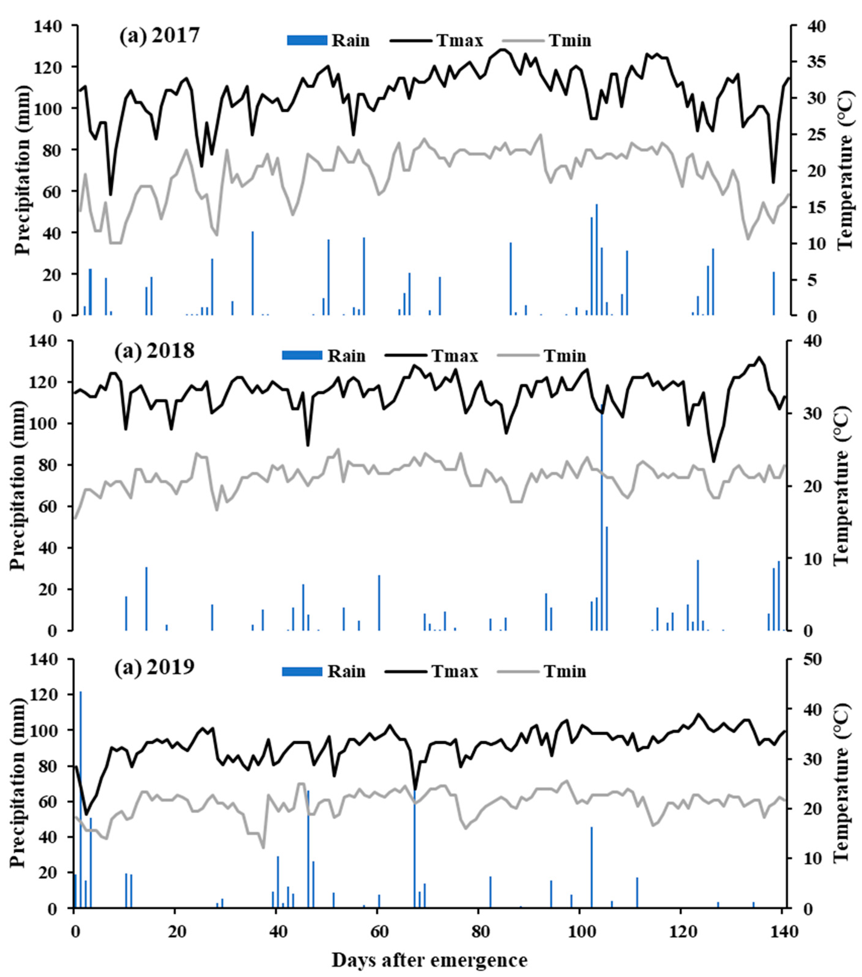
2.3. Growing Season Weather Conditions

Growing season weather data (daily maximum and minimum temperature, incoming solar radiation, and precipitation) were retrieved from the Stoneville Agricultural Weather Station located within 2 miles of the experimental site (http://deltaweather.extension.msstate.edu/, accessed on 25 February 2023) (Figure 2). For all three years, maximum and minimum air temperatures during June–August were within the range of ±2 °C of normal (Figure 2). Few extremes in air temperature were observed either in the early months, April 2017, May 2018, or late, September 2019. Rainfall distribution varied extensively throughout all three growing seasons. August was highly wet in 2017 and 2018, receiving almost four times higher than average precipitation. The growing season of 2019 received above-normal rain from May–August, receiving 227%, 177%, 138%, and 150% of average monthly rainfall, respectively.

2.4. Parametrization of Cropping System Models

Model inputs about cultural practices and crop management were similar to actual practices as stated earlier. Soybean growth and potential evapotranspiration were simulated using CSM-CROPGRO-soybean modules of DSSAT v. 4.8 [29,30] and RZWQM v. 2 [14]. For the CSM-CROPGRO-soybean model within DSSAT and RZWQM, parameters for a maturity group 4 were used for the simulation (Table 1). Soil, water, and nitrogen parameters were measured in the field or obtained from the National Cooperative Soil Survey [2], presented in

Table 2. Soil properties of Forestdale soil series used as model input for all three growing seasons.

Soil Depth (cm)	Clay %	Silt %	OC %	Total N%	pH	CEC (cmol kg−1)	θwp (cm3 cm−3)	θfc (cm3 cm−3)	θS (cm3 cm−3)	BD (Mg m−3)	KS (cm hr−1)
0–15	40.0	50.0	2.0	0.12	7.5	22.0	0.211	0.350	0.463	1.20	0.39
15–30	40.3	52.5	1.2	0.05	7.3	23.7	0.228	0.350	0.463	1.20	0.29
30–60	42.1	51.4	1.0	0.07	6.6	24.7	0.228	0.330	0.435	1.30	0.29
60–90	41.9	50.0	1.0	0.06	5.1	26.6	0.228	0.400	0.418	1.30	0.29
90–120	40.0	50.0	0.5	0.07	5.9	26.0	0.228	0.350	0.418	1.35	0.19
120–150	40.0	50.0	0.5	0.04	6.0	29.4	0.249	0.406	0.459	1.35	0.19

Notes: θ_S: saturated soil water content; θ_wp: drained soil water lower limit, θ_fc: soil water upper limit, K_S: saturated hydraulic conductivity; CEC: cation exchange capacity; BD: bulk.

.

The selection of cultivar coefficients for the simulation of soybean in three cropping system models was achieved by manually calibrating coefficients for a close match between observed and predicted values for leaf area index (LAI), grain yield, time to reach 50% flowering, and physiological maturity. Data collected in the 2017 growing season were used to calibrate model parameters, and the remaining growing seasons, 2018 and 2019, were used to evaluate the simulations. The model calibration based on the single-season data was not further modified based on the simulations obtained for the remaining two seasons.

In DSSAT and RZWQM cropping system models, crop evapotranspiration (ET_C) is calculated by initially calculating its potential rate (potential evapotranspiration, PET) under the given soil–plant–atmosphere conditions, and modifying it with actual plant uptake, transpiration, and soil–residue–crop conditions affecting evaporation from the soil surfaces [22,31,32]. In the procedure, calculated PET is first partitioned into potential soil evaporation (PE) and potential transpiration (PT) using a competing method identified by modelers involved in those modules and applied as upper limits into actual transpiration and soil evaporation loss from the system in the crop growth simulations. When multiple methods and options are available for simulations of PET in the three cropping system models, the Priestly–Taylor method with a modified ET extinction coefficient (K_ep, the coefficient used for partitioning evapotranspiration into soil and plant transpiration components) of 0.68 based on Boote et al. (2008) is used [33]. For RZWQM, the Shutterworth–Wallace [31,34] model was used to calculate potential soil evaporation (P.E.) and potential plant transpiration (P.T.). In all three models, the computed P.T. and P.E. set the upper limits for actual transpiration and actual evaporation simulated in the respective crop growth and simulation modules.

2.5. Model Performance Evaluation

The valuation of two models, CSM-CROPGRO and RZWQM, were compared based on (i) phenological growth stages, (ii) grain yield, (iii) LAI, and (iv) ET. The performance of simulation models was judged based on the root mean square error (RMSE), relative RMSE (RRMSE), percentage deviation (PD), and Nash Sutcliffe efficiency (E) using the following equations.

$$\begin{gathered} \mathrm{MSE}=\sqrt{\frac{1}{\mathrm{n}}}\sum _{\mathrm{i}=1}^{\mathrm{n}}{\left({\mathrm{P}}_{\mathrm{i}}-{\mathrm{O}}_{\mathrm{i}}\right)}^2 \\ \mathrm{RRMSE}=\frac{\mathrm{RMSE}}{{\mathrm{O}}_{\mathrm{avg}}}100 \\ \mathrm{PD}=\left\{\frac{\left({\mathrm{P}}_{\mathrm{i}}-{\mathrm{O}}_{\mathrm{i}}\right)}{{\mathrm{O}}_{\mathrm{i}}}\right\}\times 100 \\ \mathrm{E}=1-\frac{\sum _{\mathrm{i}=1}^{\mathrm{n}}{\left({\mathrm{P}}_{\mathrm{i}}-{\mathrm{O}}_{\mathrm{i}}\right)}^2}{\sum _{\mathrm{i}=1}^{\mathrm{n}}{\left({\mathrm{O}}_{\mathrm{i}}-{\mathrm{O}}_{\mathrm{avg}}\right)}^2} \end{gathered}$$

where P_i is the ith simulated value, O_i is the ith observed values, O_avg is the average of the observed values, and n is the number of data pairs.

3. Results

3.1. Phenological Stages and Grain Yield

For DSSAT, RZWQM, and three growing seasons (2017–2019), the simulated number of days from planting to seedling emergence, beginning seed, and maturity deviated from the measured values between −13 to +6 d (

Table 3. Measured (M), simulated (S), and error (S-M) for critical phenological growth stages (in days after planting, DAP), grain yield, and ET_C of soybean during the 2017–2019 growing seasons.

Parameters	Measured (M)		DSSAT		RZWQM
	Day	DAP	S	Error	S	Error
2017
Emergence	28 April	7	7	0	8	1
First flower	28 May	37	42	5
First pod	27 June	67	56	−11	62	2
First seed	15 July	85	72	−13	85	0
Physiological maturity	7 September	139	134	−5	142	3
Grain yield (kg ha−1)	4771		4843	72	5057	286
Average daily ETC (mm)	4.71		4.38	−0.33	4.66	−0.05
Cumulative ETC (mm)	584		544	−40	577	−7
2018
Emergence	7 May	9	6	−3	8	−1
First flower	9 June	42	35	−7
First pod	22 June	55	49	−6	56	1
First seed	9 July	72	65	−7	76	4
Physiological maturity	12 September	137	125	−12	136	−1
Grain yield (kg ha−1)	5783		4399	−1384	5423	−360
Average daily ETC (mm)	4.84		4.55	−0.29	4.42	−0.42
Cumulative ETC	532		501	−31	486	−46
2019
Emergence	8 May	7	6	−1	8	1
First flower	13 June	43	37	−6
First pod	22 June	52	52	0	58	6
First seed	11 July	71	68	−3	77	6
Physiological maturity	14 September 2019	136	128	−8	136	0
Grain yield (kg ha−1)	4909		4986	77	5399	490
Average daily ETC (mm)	4.64		4.41	−0.23	4.40	−0.24
Cumulative ETC	566		550	−16	537	−29

). Over cropping seasons, the simulation of the number of days from seed planting to emergence deviated from measured values from −3 to −1 d for DSSAT and ±1 d for RZWQM. Beginning seed formation (R5) varied from −3 to −13 d for DSSAT and −1 to 6 d for RZWQM. Finally, maturity varied from −5 to −12 d for DSSAT, and −1 to 3 d for RZWQM. Grain yield ranged from 72 to −1384 kg ha⁻¹ for DSSAT, and −360 to 490 kg ha⁻¹ for RZWQM.

3.2. LAI

The maximum observed LAI values were 5.2, 5.8, and 5.8 observed on 102 d, 107 d, and 88 d after emergence (DAE) for 2017, 2018, and 2019 seasons, respectively (Figure 3). In 2017, DSSAT and RZWQM simulated maximum LAI values of 5.82 and 6.10, observed on 70 DAE and 71 DAE, respectively. The simulation of LAI with DSSAT and RZWQM resulted in RRMSE values of 45.0% and 37.8%, respectively. In 2018, DSSAT and RZWQM simulated maximum values were 5.71 (65 on DAE) and 6.08 (on 68 DAE), with corresponding RMSE values of 1.30 and 1.05, respectively. The simulation of LAI with DSSAT and RZWQM resulted in RRMSE values of 34.5% and 27.8%, respectively. In 2019, DSSAT and RZWQM predicted maximum LAI values of 5.85 (on 67 DAE) and 6.14 (on 67 DAE), respectively. The RRMSE values for DSSAT and RZWQM were 17.9% and 17.0%, respectively.

3.3. Crop Evapotranspiration (ET_C)

In 2017, the cumulative ET_C value using the EC method was 584 mm. In contrast, the simulated values were 544 mm and 577 mm for DSSAT and RZWQM, respectively (Figure 4). The average observed daily ET_C value was 4.71 mm, and DSSAT and RZWQM predicted 4.38 mm and 4.66 mm, respectively. The highest observed ET_C was 7.75 mm; DSSAT, and RZWQM had the highest values of 7.19 and 8.08 mm, respectively. For DSSAT and RZWQM, the RMSE values were 1.96 mm and 1.39 mm, with corresponding RRMSE values of 41.6% and 29.6%, respectively.

In 2018, the cumulative ET_C value quantified using the EC method was 532 mm, whereas the predicted values were 501 mm and 486 mm for DSSAT and RZWQM, respectively. The average observed daily ET_C values were 4.84 mm, when DSSAT and RZWQM predicted 4.55 mm and 4.42 mm, respectively. The highest observed daily ET_C was 7.69 mm, whereas DSSAT and RZWQM simulations had the highest daily ET_C values of 7.26 mm and 9.69 mm, respectively. DSSAT and RZWQM had RMSE and RRMSE values of 1.82 and 37.7%, and 2.13 and 44.0%, respectively.

In 2019, the cumulative ET_C was 566 mm, and the simulated values were 550 mm and 537 mm for DSSAT and RZWQM, respectively. The average observed daily ET_C was 4.64 mm, but the average simulated values were 4.41 mm and 4.40 mm for DSSAT and RZWQM, respectively. The highest observed ET_C value was 7.61 mm, while DSSAT and RZWQM had the highest simulated values of 7.21 mm and 9.49 mm, respectively. Two models had RMSE and RRMSE values of 2.14 and 46.0%, and 2.56 and 55.1%, for DSSAT and RZWQM, respectively.

Considering all three growing seasons, the observed average daily ET_C was 4.73 mm, where the DSSAT and RZWQM simulated values were 4.44 mm and 4.49 mm, respectively. The three-year average of observed cumulative ET_C was 560 mm, and for DSSAT and RZWQM the simulated values were 532 mm and 533 mm, respectively.

4. Discussion

As expected in simulating crop phenology, grain yield, and ET_C in response to management and weather information, the simulated soybean phenology and grain yield deviated from the measured values but within the error limits commonly reported in the literature [4,35]. In this investigation, simulating the soybean crop growth during 2017–2019 in the humid LMD region, the extent of deviations of simulated processes depended on the particular model used and growing season characteristics. The weather data showed that the amount and distribution of rainfall varied extensively during the three growing seasons. During the wet years, high-intensity precipitation events increase run off, water infiltrations and deep drainage losses. When such large variations in weather during the crop growth season drive the cropping system simulation models, it becomes extremely difficult for accurate crop growth simulations. However, such errors typically observed are comparable to the extent of errors that can occur in the precise quantification of those natural processes. This is usually reflected in crop simulation results.

For simulating crop growth and yield, accurate simulations of crop phenology are desired [36]. In soybean growth simulations using two cropping system models in this study, simulated crop phenology controls most crop physiological processes such as leaf area, biomass accumulation and partitioning, and biological N fixation [15]. Indeterminate soybean varieties showed considerable overlap between visual growth stages; as such, observations usually are subjected to substantial human error. Simulations of growth stages, that is, seedling emergence from the soil, first flower, beginning seed, and physiological maturity, showed an overall variation of −13 to +6 d (Table 3). However, the magnitude of errors in phenological simulations did not reflect the same extent in ETC and grain yield (Table 3).

For the grain yield prediction, both models overpredict grain yields during 2017 and 2019 and underpredict grain yield for 2018. Using RZWQM v 2.0, Anapalli et al. (2019) reported an overestimation of simulated grain yield data collected for other locations in the LMD by 283 (5%) kg ha⁻¹ and 727 kg ha⁻¹ (+15%) during the 2016 and 2017 growing seasons, respectively [14]. Battisti et al. (2018) observed that the soybean grain yield prediction had a higher rate of reduction when rainfall was diminished than when rainfall was increased when comparing four models, AQUACROP, MONICA, DSSAT, and APSIM, in Southern Brazil [20].

Both crop models simulated LAI values that closely followed observed values from emergence to 40 DAE, but overpredicted LAI during 53–78, 48–78, and 58–78 DAE during 2017, 2018, and 2019, respectively. Over time, soybean cultivars have changed rapidly in their genetic makeup and growth traits, which respond differently to the amount of available water for plant uptake and the stress induced on plant growth processes from a deficit or excess of water [36].

Overestimation of LAI might be associated with overestimating ET_C, particularly during the reproductive growth phase. Da Silva et al. (2022) also observed an overprediction of E.T. late during the growing season [21]. They attributed the outcome to an overestimation of LAI between 60–100 days after planting (DAP) for Priestly–Taylor and FAO56 Pennman–Monteith PET methods for the CSM-CROPGRO-soybean model. Singer et al. (2010) found that the E + T method overestimated E.T. from 0.68 to 1.58 mm when comparing evaporation plus transpiration versus ET_C from the eddy covariance system [7]. For corn, soybean, and cotton cropping systems in the LMD, Anapalli et al. (2019) found RMSEs between 0.9 and 1.4 mm and RRMSEs between 21 and 37% between the simulated daily ET_C from EC and energy balance estimates, due to 2 to 12% of the variation in incoming and outgoing energies in the EC system [14]. Several studies [1,3,37] emphasized that the crop coefficient (K_C) often showed considerable variation from FAO-56 values due to wetting events and suggested improvement in K_C values for the irrigated system due to frequent soil surface wetting by rain or irrigation.

5. Conclusions

This study emphasized the evaluation of cropping system models for simulations of ET_C over multiple growing seasons. Cropping system models help predict crop ET_C from location-specific weather–soil–crop management information to develop tactical and strategic water management decision support data for optimizing location-specific crop water use. We evaluated the DSSAT and RZWQM models for simulations of ET_C against those quantified using the EC method. Seasonal cumulative ET_C simulations by both models compared well with EC measurements. The two models evaluated were seen to carry a high potential for strategic water management in irrigated production systems. Due to the indeterminate growth habits of the soybean crop, the evaluation of phenology simulations across models is often challenging. Besides accurate ET_C measurements and soil properties, datasets should include profile soil moisture measurements and in-season biomass accumulation over several growth stages to capture the water dynamics in the system arising out of varying rainfall distributions within and across crop seasons. However, the study revealed that the two models evaluated have a high potential for applications in sustainable water management decision support development in field crop agriculture.

References

1. Anapalli, S.S.; Krutz, J.L.; Pinnamaneni, S.R.; Reddy, K.N.; Fisher, D.K. Eddy covariance quantification of soybean (Glycine max L.) crop coefficients in a farmer’s field in a humid climate. Irrig. Sci. 2021, 39, 651–669. [Google Scholar] [CrossRef]
2. National Cooperative Soil Survey (NCSS) Advanced Query, National Cooperative Soil Survey Soil Characterization Database. Available online: https://ncsslabdatamart.sc.egov.usda.gov/advquery.aspx (accessed on 25 August 2023).
3. Payero, J.O.; Irmak, S. Daily energy fluxes, evapotranspiration and crop coefficient of soybean. Agric. Water Manag. 2013, 129, 31–43. [Google Scholar] [CrossRef]
4. Kimball, B.A.; Boote, K.J.; Hatfield, J.L.; Ahuja, L.R.; Stockle, C.; Archontoulis, S.; Baron, C.; Basso, B.; Bertuzzi, P.; Constantin, J.; et al. Simulation of maize evapotranspiration: An inter-comparison among 29 maize models. Agric. Water Manag. 2019, 271, 264–284. [Google Scholar] [CrossRef]
5. Tang, Q.; Feng, G.; Fisher, D.; Zhang, H.; Ouyang, Y.; Adeli, A.; Jenkins, J. Rain Water Deficit and Irrigation Demand of Major Row Crops in the Mississippi Delta. T Asabe 2018, 61, 927–935. [Google Scholar] [CrossRef]
6. Runkle, B.R.K.; Rigby, J.R.; Reba, M.L.; Anapalli, S.S.; Bhattacharjee, J.; Krauss, K.W.; Liang, L.; Locke, M.A.; Novick, K.A.; Sui, R.X.; et al. Delta-Flux: An Eddy Covariance Network for a Climate-Smart Lower Mississippi Basin. Agric. Environ. Lett. 2017, 2, ael2017.01.0003. [Google Scholar] [CrossRef]
7. Singer, J.W.; Heitman, J.L.; Hernandez-Ramirez, G.; Sauer, T.J.; Prueger, J.H.; Hatfield, J.L. Contrasting methods for estimating evapotranspiration in soybean. Agric. Water Manag. 2010, 98, 157–163. [Google Scholar] [CrossRef]
8. Rana, G.; Katerji, N. Measurement and estimation of actual evapotranspiration in the field under Mediterranean climate: A review. Eur. J. Agron. 2000, 13, 125–153. [Google Scholar] [CrossRef]
9. Farahani, H.J.; Howell, T.A.; Shuttleworth, W.J.; Bausch, W.C. Evapotranspiration: Progress in measurement and modeling in agriculture. Trans. Asabe 2007, 50, 1627–1638. [Google Scholar] [CrossRef]
10. Wang, K.C.; Dickinson, R.E. A Review of Global Terrestrial Evapotranspiration: Observation, Modeling, Climatology, and Climatic Variability. Rev. Geophys. 2012, 50. [Google Scholar] [CrossRef]
11. Ghiat, I.; Mackey, H.R.; Al-Ansari, T. A Review of Evapotranspiration Measurement Models, Techniques and Methods for Open and Closed Agricultural Field Applications. Water 2021, 13, 2523. [Google Scholar] [CrossRef]
12. Talib, A.; Desai, A.R.; Huang, J.Y.; Griffis, T.J.; Reed, D.E.; Chen, J.Q. Evaluation of prediction and forecasting models for evapotranspiration of agricultural lands in the Midwest U.S. J. Hydrol. 2021, 600, 126579. [Google Scholar] [CrossRef]
13. Li, Z.L.; Tang, R.L.; Wan, Z.M.; Bi, Y.Y.; Zhou, C.H.; Tang, B.H.; Yan, G.J.; Zhang, X.Y. A Review of Current Methodologies for Regional Evapotranspiration Estimation from Remotely Sensed Data. Sensors 2009, 9, 3801–3853. [Google Scholar] [CrossRef] [PubMed]
14. Anapalli, S.S.; Fisher, D.K.; Reddy, K.N.; Rajan, N.; Pinnamaneni, S.R. Modeling evapotranspiration for irrigation water management in a humid climate. Agric. Water Manag. 2019, 225, 105731. [Google Scholar] [CrossRef]
15. Wu, Y.S.; Wang, E.L.; He, D.; Liu, X.; Archontoulis, S.V.; Huth, N.I.; Zhao, Z.G.; Gong, W.Z.; Yang, W.Y. Combine observational data and modelling to quantify cultivar differences of soybean. Eur. J. Agron. 2019, 111, 125940. [Google Scholar] [CrossRef]
16. Yang, X.; Zheng, L.N.; Yang, Q.; Wang, Z.K.; Cui, S.; Shen, Y.Y. Modelling the effects of conservation tillage on crop water productivity, soil water dynamics and evapotranspiration of a maize-winter wheat-soybean rotation system on the Loess Plateau of China using APSIM. Agric. Syst. 2018, 166, 111–123. [Google Scholar] [CrossRef]
17. Allen, R.G.; Pereira, L.S.; Raes, D.; Smith, M. Crop evapotranspiration-Guidelines for computing crop water requirements-FAO Irrigation and drainage paper 56. Fao 1998, 300, D05109. [Google Scholar]
18. Priestley, C.H.B.; Taylor, R.J. On the assessment of surface heat flux and evaporation using large-scale parameters. Mon. Weather Rev. 1972, 100, 81–92. [Google Scholar] [CrossRef]
19. Monteith, J.L. Evaporation and environment. Symp. Soc. Exp. Biol. 1965, 19, 205–234. [Google Scholar]
20. Battisti, R.; Sentelhas, P.C.; Boote, K.J. Sensitivity and requirement of improvements of four soybean crop simulation models for climate change studies in Southern Brazil. Int. J. Biometeorol. 2018, 62, 823–832. [Google Scholar] [CrossRef]
21. da Silva, E.H.F.M.; Hoogenboom, G.; Boote, K.J.; Gonsalves, A.O.; Marin, F.R. Predicting soybean evapotranspiration and crop water productivity for a tropical environment using the CSM-CROPGRO-Soybean model. Agric. For. Meteorol. 2022, 323, 109075. [Google Scholar] [CrossRef]
22. Anapalli, S.S.; Ahuja, L.R.; Gowda, P.H.; Ma, L.W.; Marek, G.; Evett, S.R.; Howell, T.A. Simulation of crop evapotranspiration and crop coefficients with data in weighing lysimeters. Agric. Water Manag. 2016, 177, 274–283. [Google Scholar] [CrossRef]
23. Hodges, T.; French, V. Soyphen—Soybean Growth-Stages Modeled from Temperature, Daylength, and Water Availability. Agron. J. 1985, 77, 500–505. [Google Scholar] [CrossRef]
24. Isaac, P.; Cleverly, J.; McHugh, I.; Van Gorsel, E.; Ewenz, C.; Beringer, J. OzFlux data: Network integration from collection to curation. Biogeosciences 2017, 14, 2903–2928. [Google Scholar] [CrossRef]
25. Mauder, M.; Foken, T. Impact of post-field data processing on eddy covariance flux estimates and energy balance closure. Meteorol. Z. 2006, 15, 597–609. [Google Scholar] [CrossRef]
26. Fratini, G.; McDermitt, D.K.; Papale, D. Eddy-covariance flux errors due to biases in gas concentration measurements: Origins, quantification and correction. Biogeosciences 2014, 11, 1037–1051. [Google Scholar] [CrossRef]
27. De Roo, F.; Zhang, S.; Huq, S.; Mauder, M. A semi-empirical model of the energy balance closure in the surface layer. PLoS ONE 2018, 13, e0209022. [Google Scholar] [CrossRef] [PubMed]
28. Reichstein, M.; Falge, E.; Baldocchi, D.; Papale, D.; Aubinet, M.; Berbigier, P.; Bernhofer, C.; Buchmann, N.; Gilmanov, T.; Granier, A.; et al. On the separation of net ecosystem exchange into assimilation and ecosystem respiration: Review and improved algorithm. Glob. Change Biol. 2005, 11, 1424–1439. [Google Scholar] [CrossRef]
29. Hoogenboom, G.; Porter, C.H.; Shelia, V.; Boote, K.J.; Singh, U.; White, J.W.; Pavan, W.; Oliveira, F.A.A.; Moreno-Cadena, L.P.; Lizaso, J.I.; et al. Decision Support System for Agrotechnology Transfer (DSSAT) Version <4.8>; DSSAT Foundation: Gainesville, FL, USA, 2021. [Google Scholar]
30. Jones, J.W.; Hoogenboom, G.; Porter, C.H.; Boote, K.J.; Batchelor, W.D.; Hunt, L.A.; Wilkens, P.W.; Singh, U.; Gijsman, A.J.; Ritchie, J.T. The DSSAT cropping system model. Eur. J. Agron. 2003, 18, 235–265. [Google Scholar] [CrossRef]
31. Ahuja, L.; Ma, L. Parameterization of Agricultural System Models: Current Approaches and Future Needs. Agricultural System Models in Field Research and Technology Transfer; Lewis Publishers: Boca Raton, FL, USA, 2002. [Google Scholar]
32. Ritchie, J.T. Model for predicting evaporation from a row crop with incomplete cover. Water Resour. Res. 1972, 8, 1204–1213. [Google Scholar] [CrossRef]
33. Boote, K.; Sau, F.; Hoogenboom, G.; Jones, J.W. Experience with water balance, evapotranspiration, and predictions of water stress effects in the CROPGRO model. Response Crops Ltd. Water Underst. Model. Water Stress Eff. Plant Growth Process. 2008, 1, 59–103. [Google Scholar]
34. Shuttleworth, W.J.; Wallace, J.S. Evaporation from Sparse Crops—An Energy Combination Theory. Q. J. R. Meteor. Soc. 1985, 111, 839–855. [Google Scholar] [CrossRef]
35. Bassu, S.; Brisson, N.; Durand, J.L.; Boote, K.; Lizaso, J.; Jones, J.W.; Rosenzweig, C.; Ruane, A.C.; Adam, M.; Baron, C.; et al. How do various maize crop models vary in their responses to climate change factors? Glob. Change Biol. 2014, 20, 2301–2320. [Google Scholar] [CrossRef] [PubMed]
36. Archontoulis, S.V.; Miguez, F.E.; Moore, K.J. A methodology and an optimization tool to calibrate phenology of short-day species included in the APSIM PLANT model: Application to soybean. Environ. Model. Softw. 2014, 62, 465–477. [Google Scholar] [CrossRef]
37. Anapalli, S.S.; Fisher, D.K.; Reddy, K.N.; Wagle, P.; Gowda, P.H.; Sui, R. Quantifying soybean evapotranspiration using an eddy covariance approach. Agric. Water Manage 2018, 209, 228–239. [Google Scholar] [CrossRef]
Figure 1. Eddy covariance unit with sensor cluster positioned 2 m above the canopy centrally located in a large farm-scale soybean field.
Water 15 03078 g001
Figure 2. Daily rainfall distribution and changes in maximum (Tmax) and minimum (Tmin) air temperature during the 2017–2019 growing seasons (reproduced with permission from Annapalli et al., 2021) [1].
Water 15 03078 g002
Figure 3. Changes in measured and simulated (DSSAT and RZWQM models) leaf area index (LAI) during (a) 2017, (b) 2018, and (c) 2019 growing seasons of the soybean production system.
Water 15 03078 g003
Figure 4. Daily and cumulative seasonal evapotranspiration (ETC) measured with eddy covariance (EC) and predictions of DSSAT and RZWQM for calibration and evaluation during (a,b) 2017, (c,d) 2018, and (e,f) 2019 growing seasons.
Water 15 03078 g004