

Extreme Runoff Estimation for Ungauged Watersheds Using a New Multisite Multivariate Stochastic Model MASVC
Abstract
:1. Introduction
2. Materials and Methods
2.1. Multisite Multivariate Stochastic Model MASVC
2.2. Probability Density Functions (PDF)
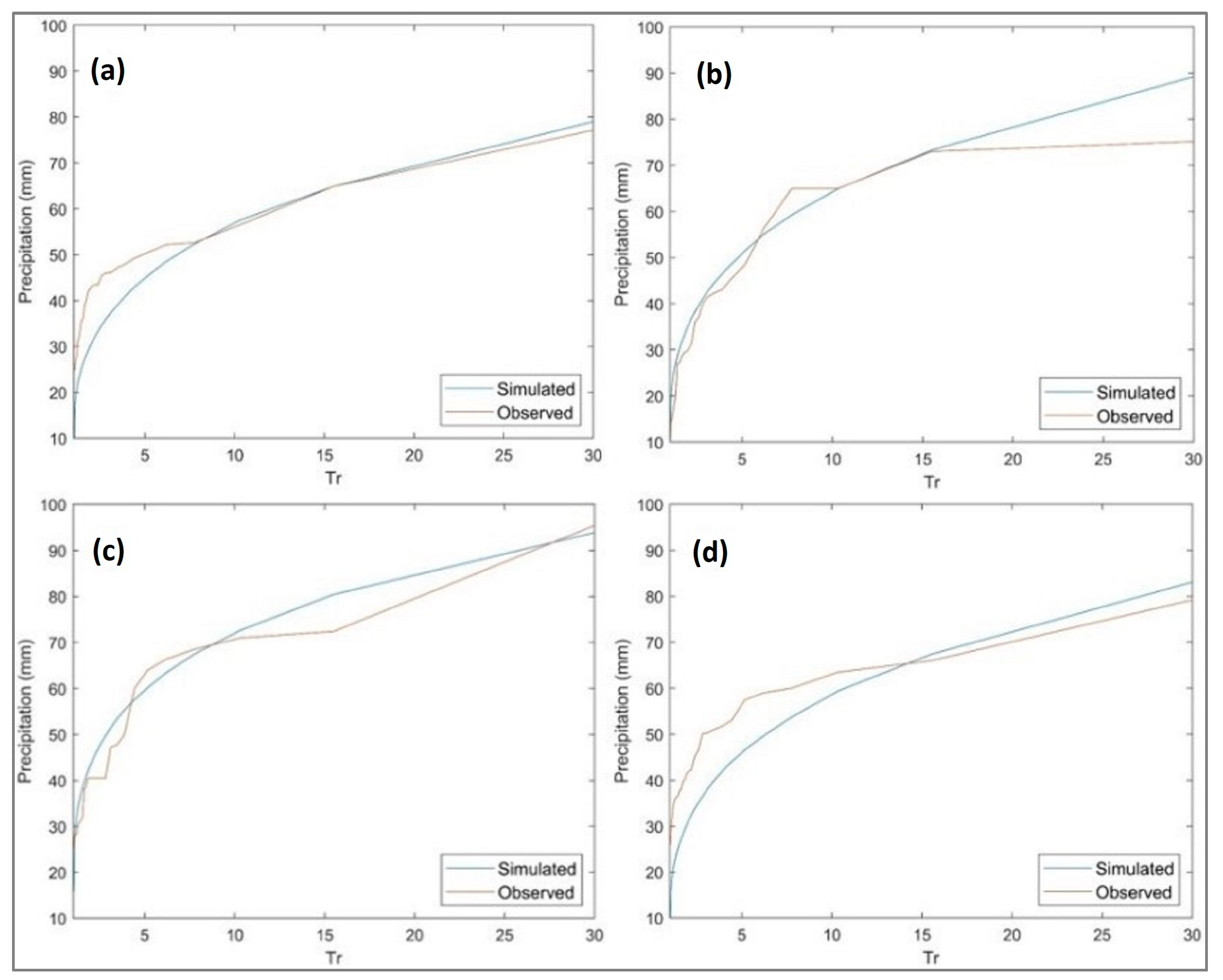
2.3. Curves IDT
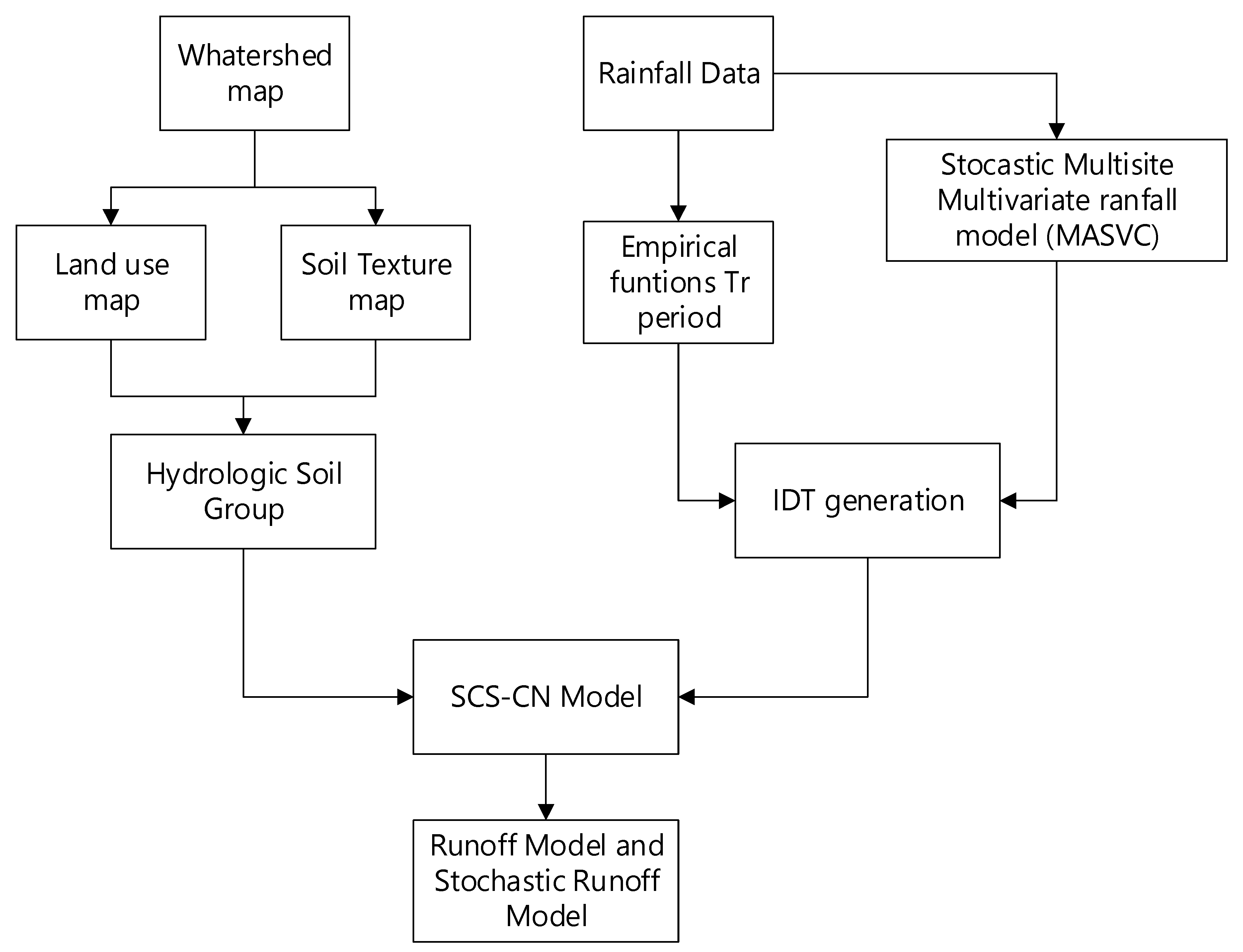
2.4. Soil Conservation Service Curve Number Method (SCS-CN)
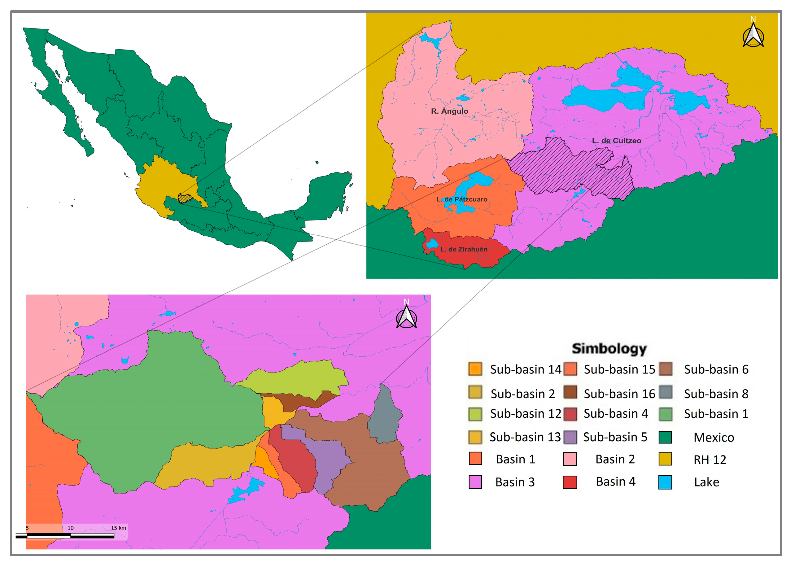
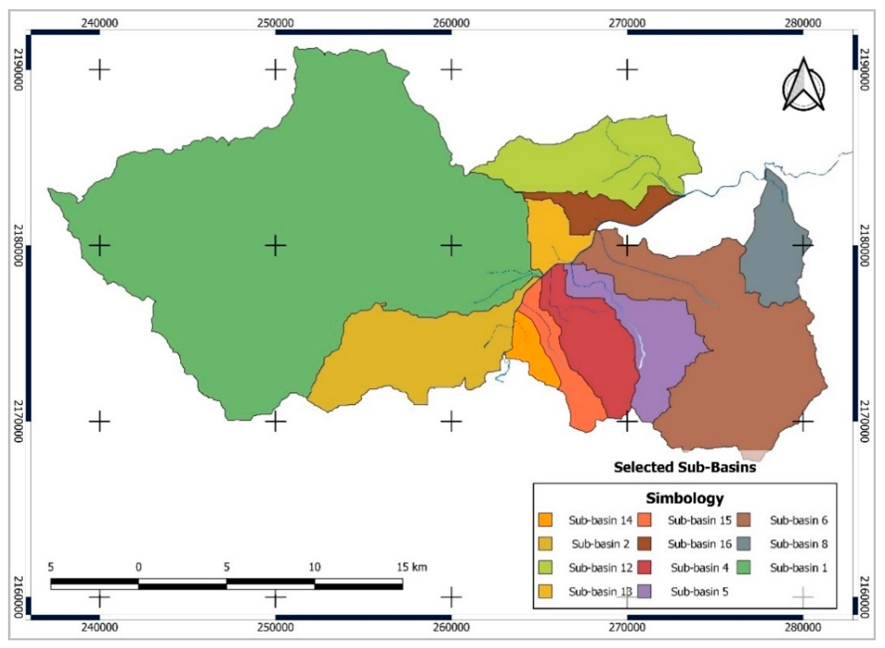
2.5. Case Study
3. Results
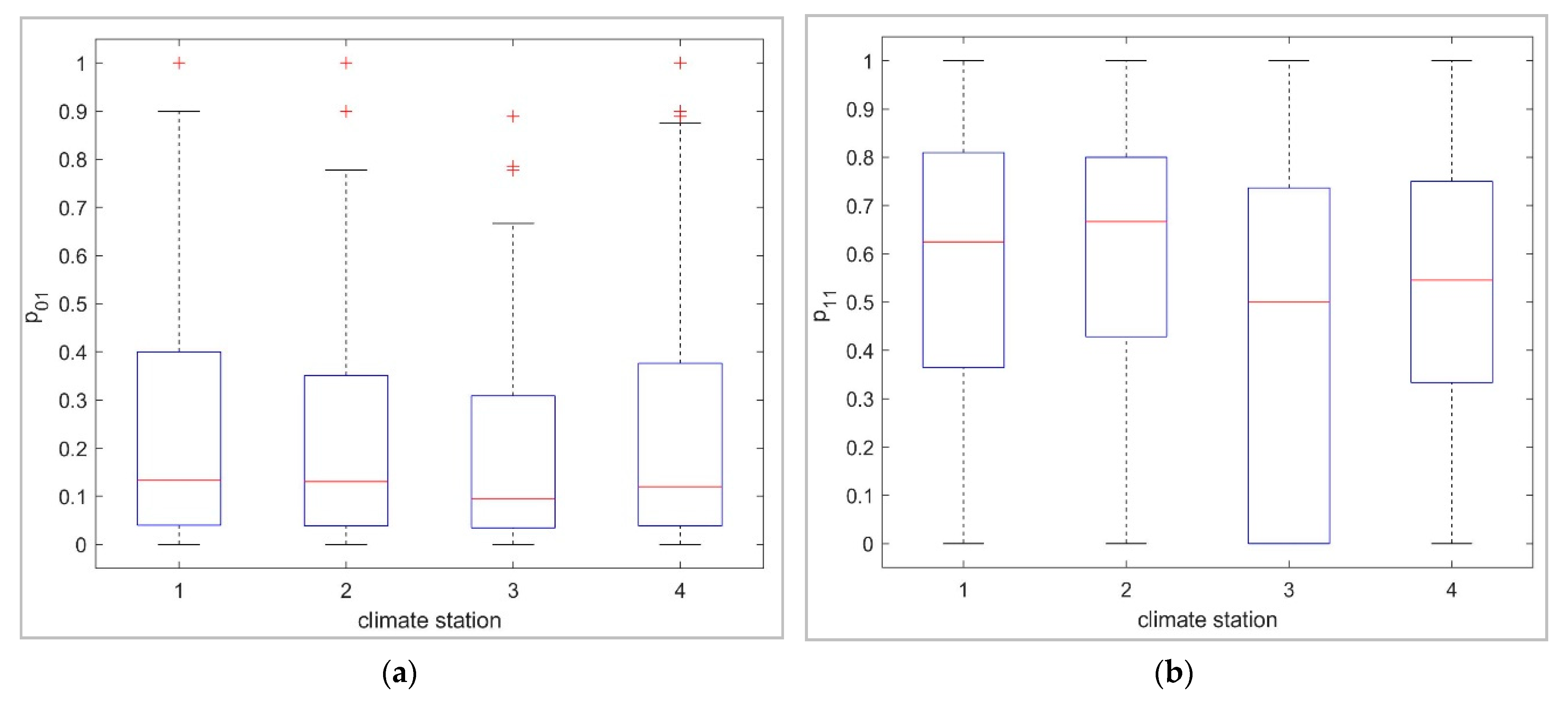
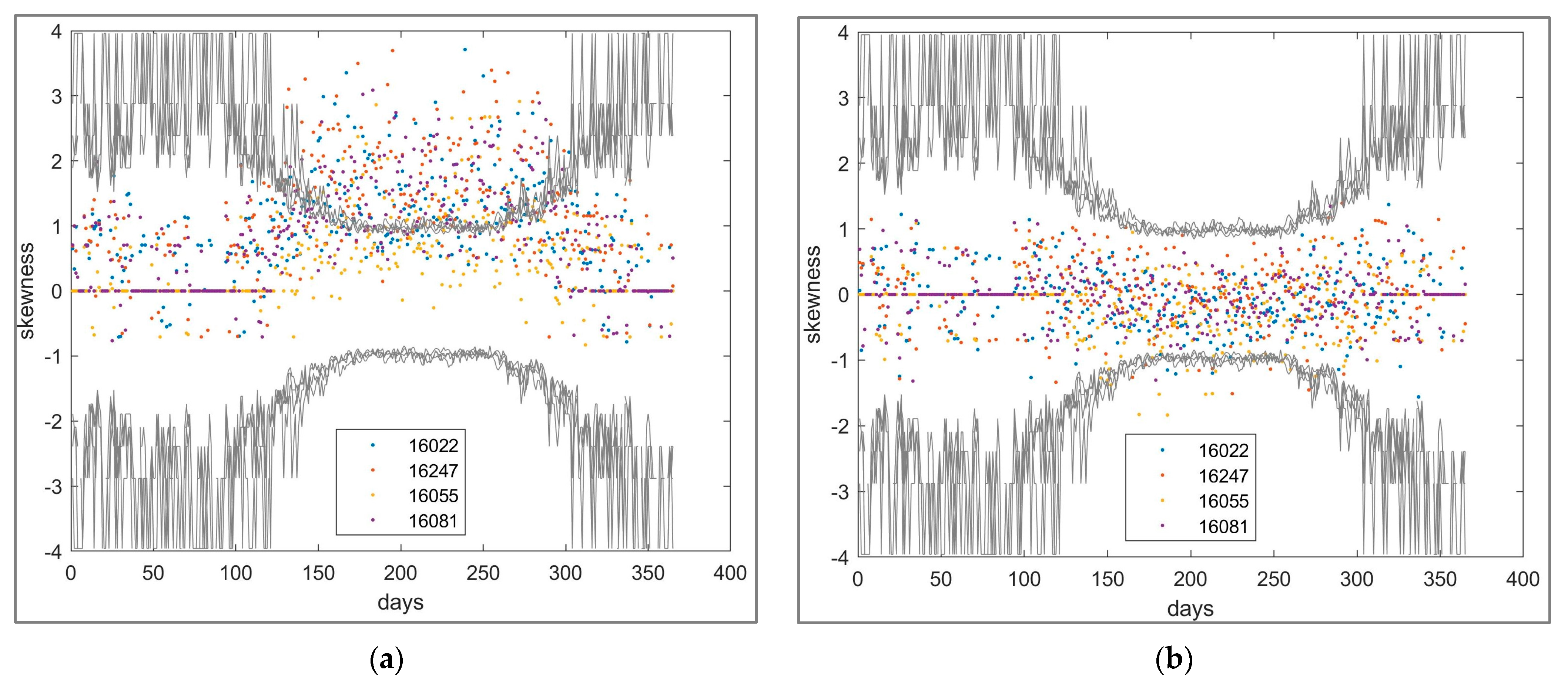
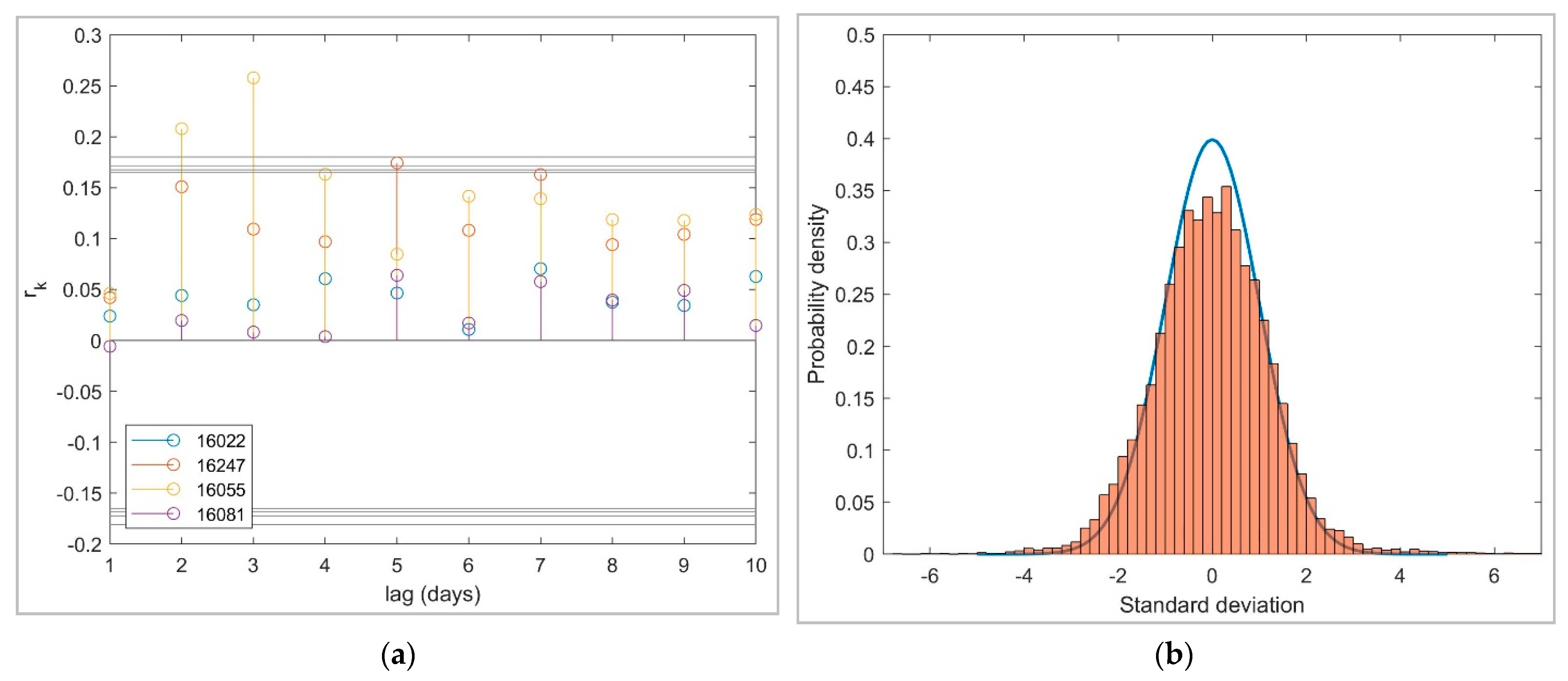
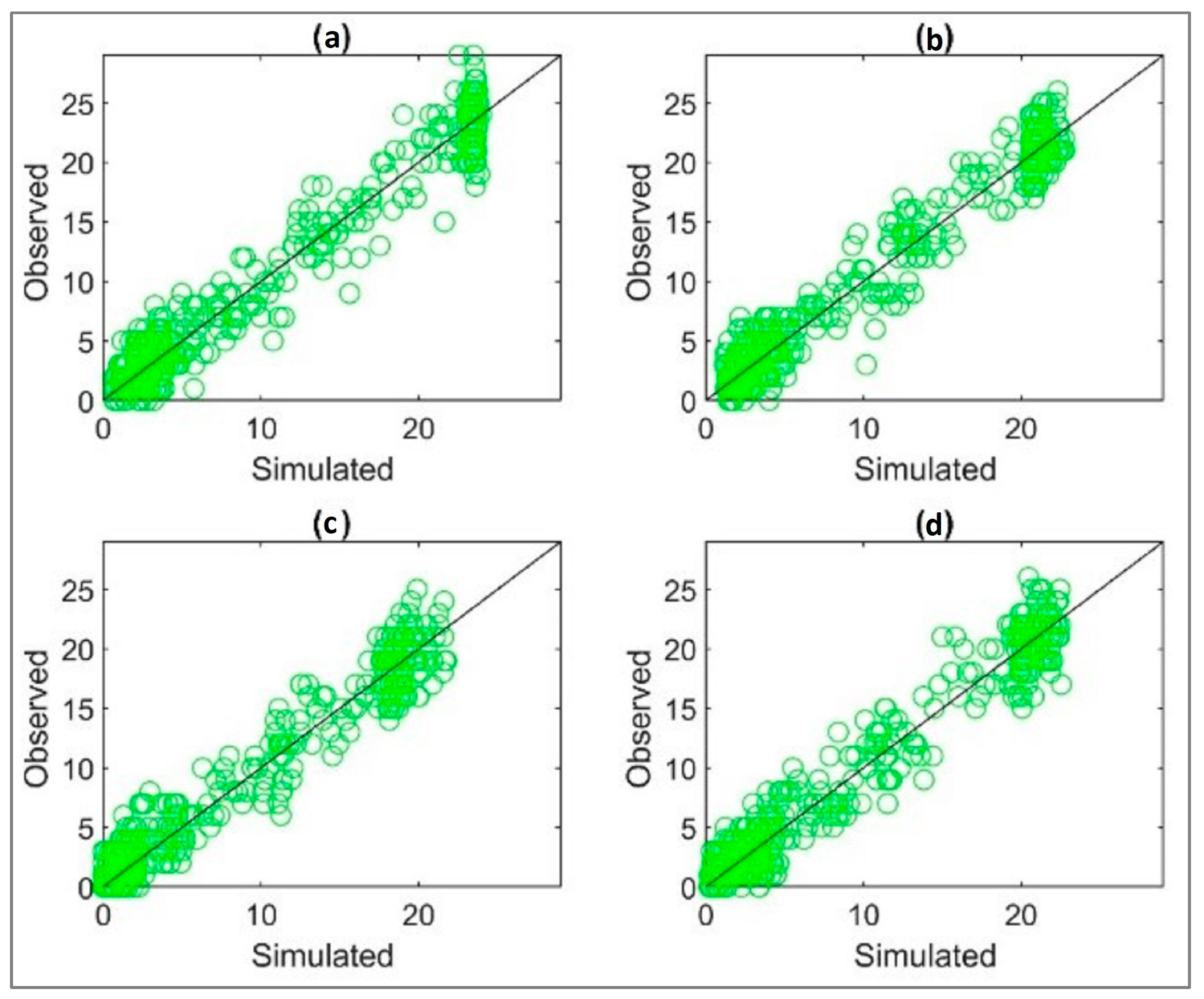
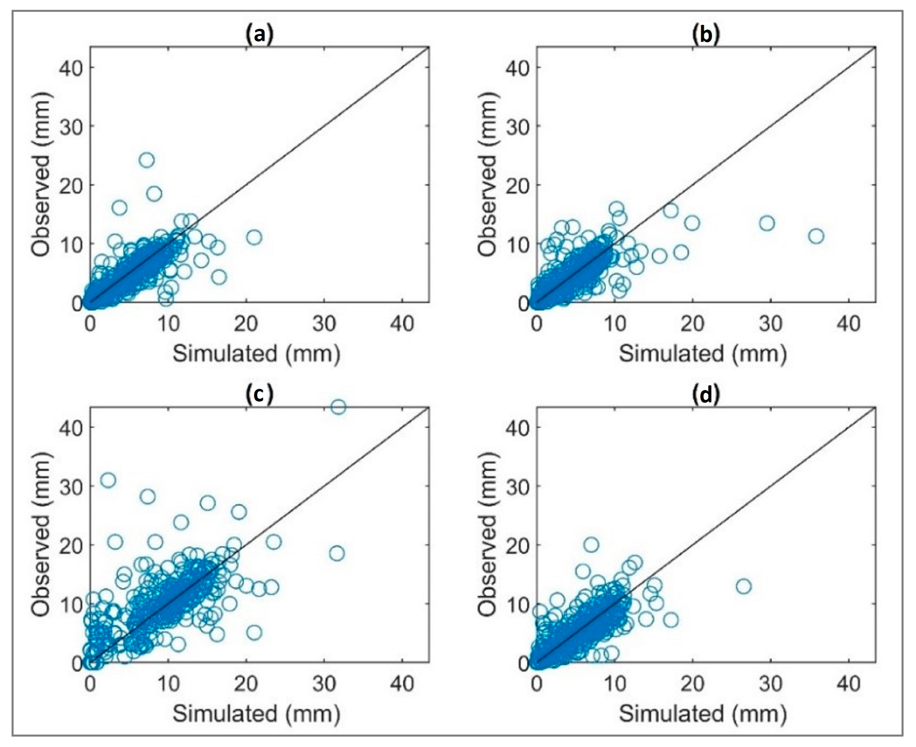
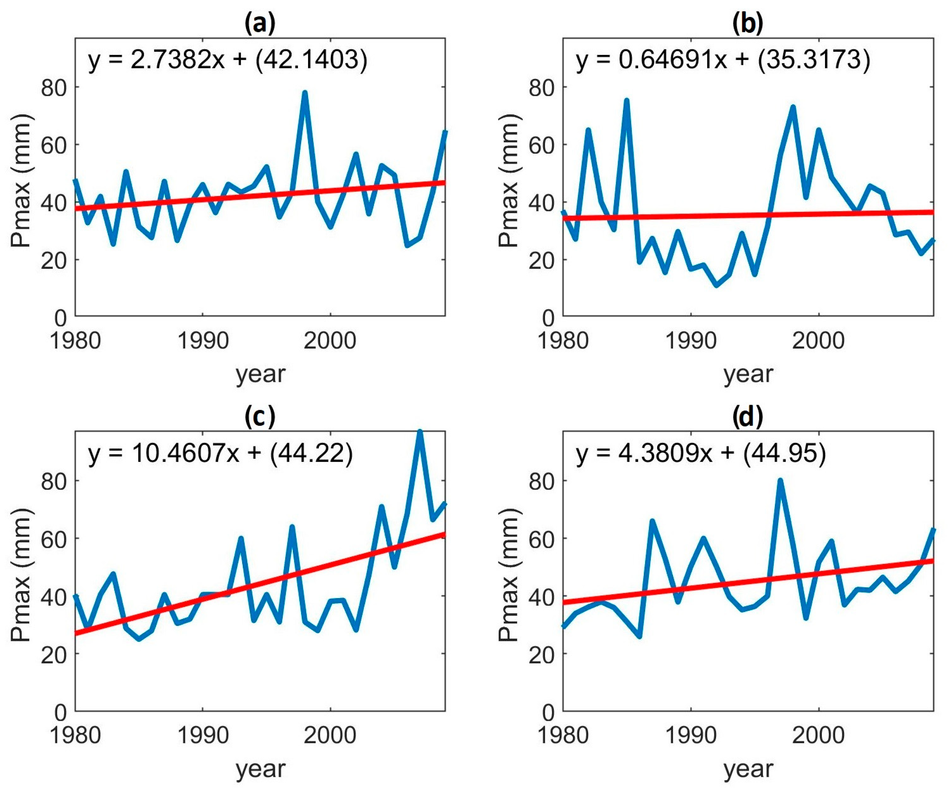
3.1. Multisite Multivariate Stochastic Results
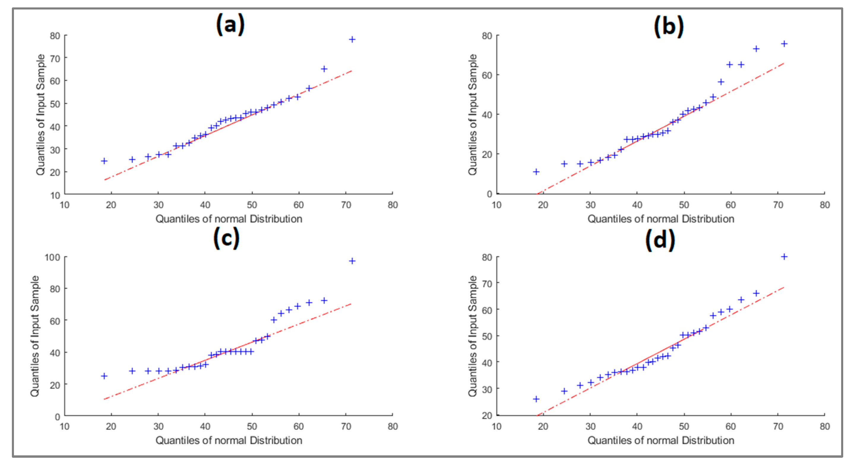
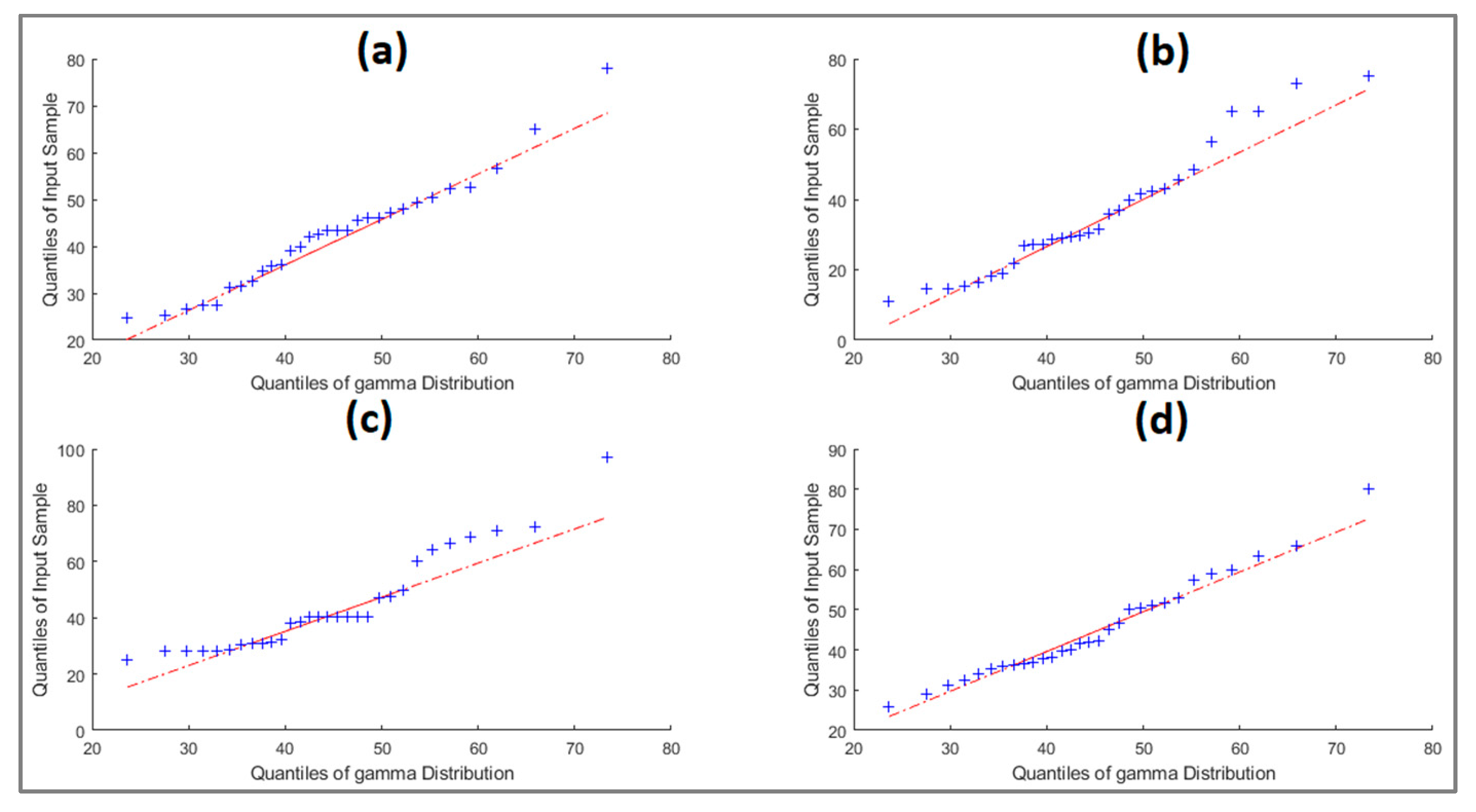
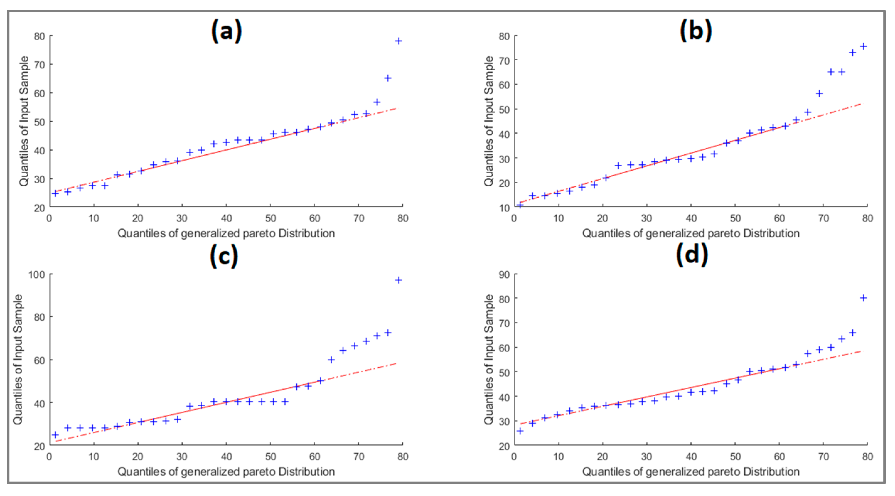
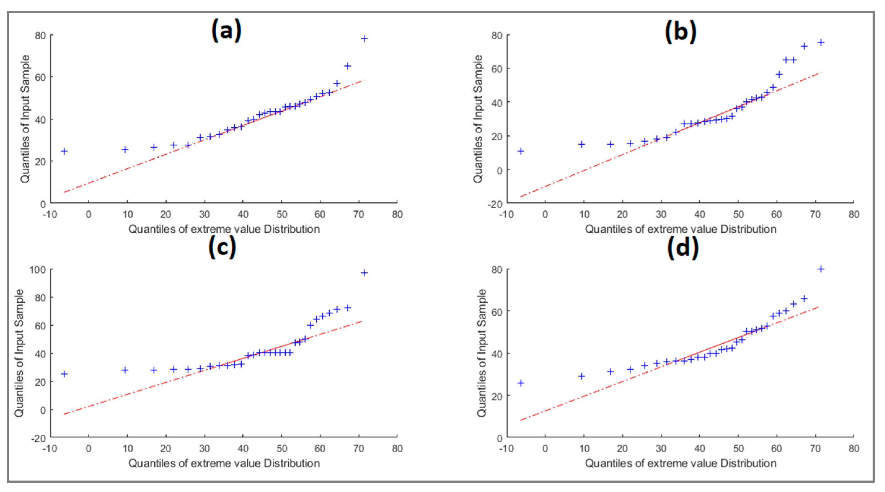
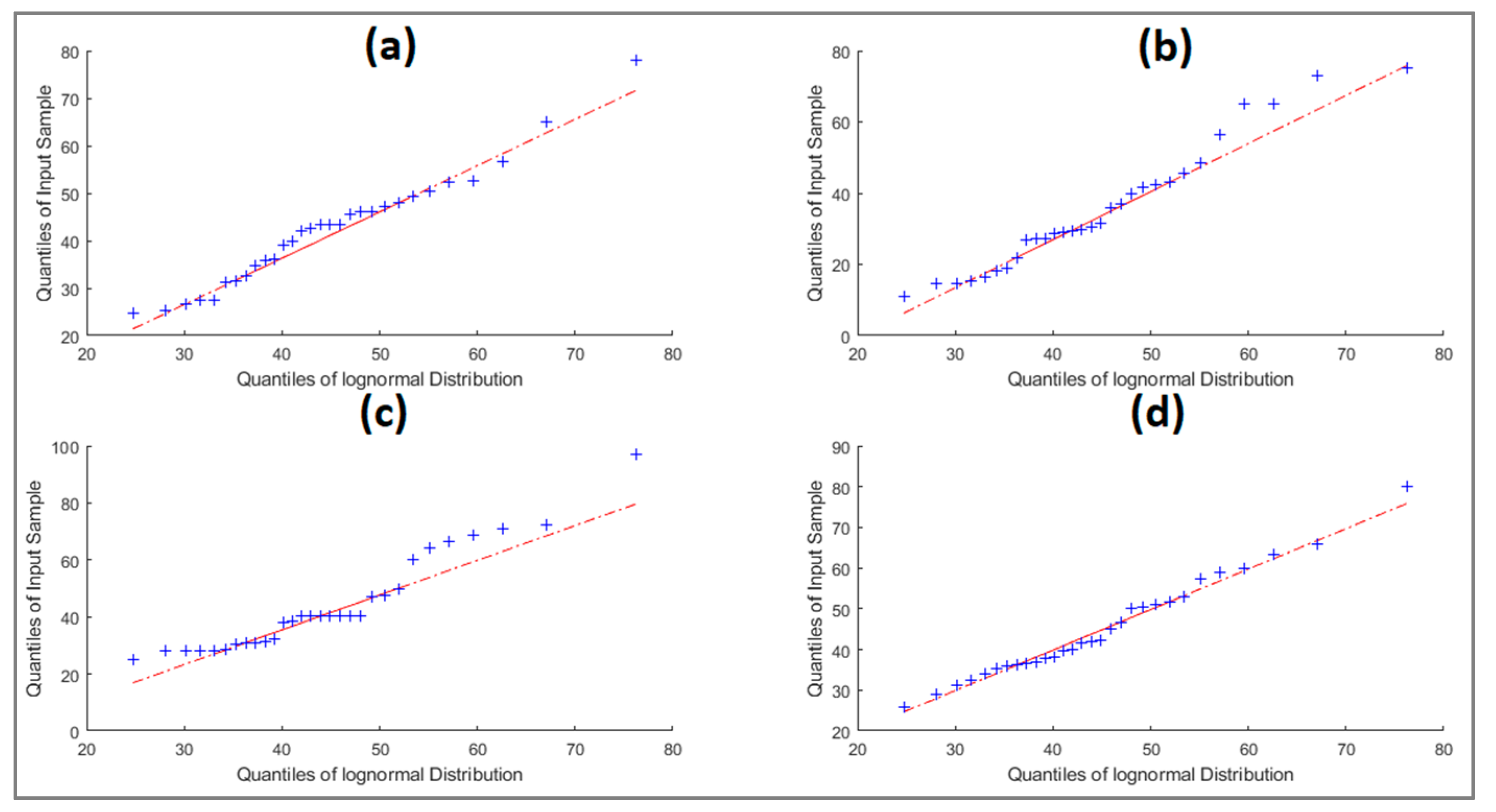
3.2. PDFs
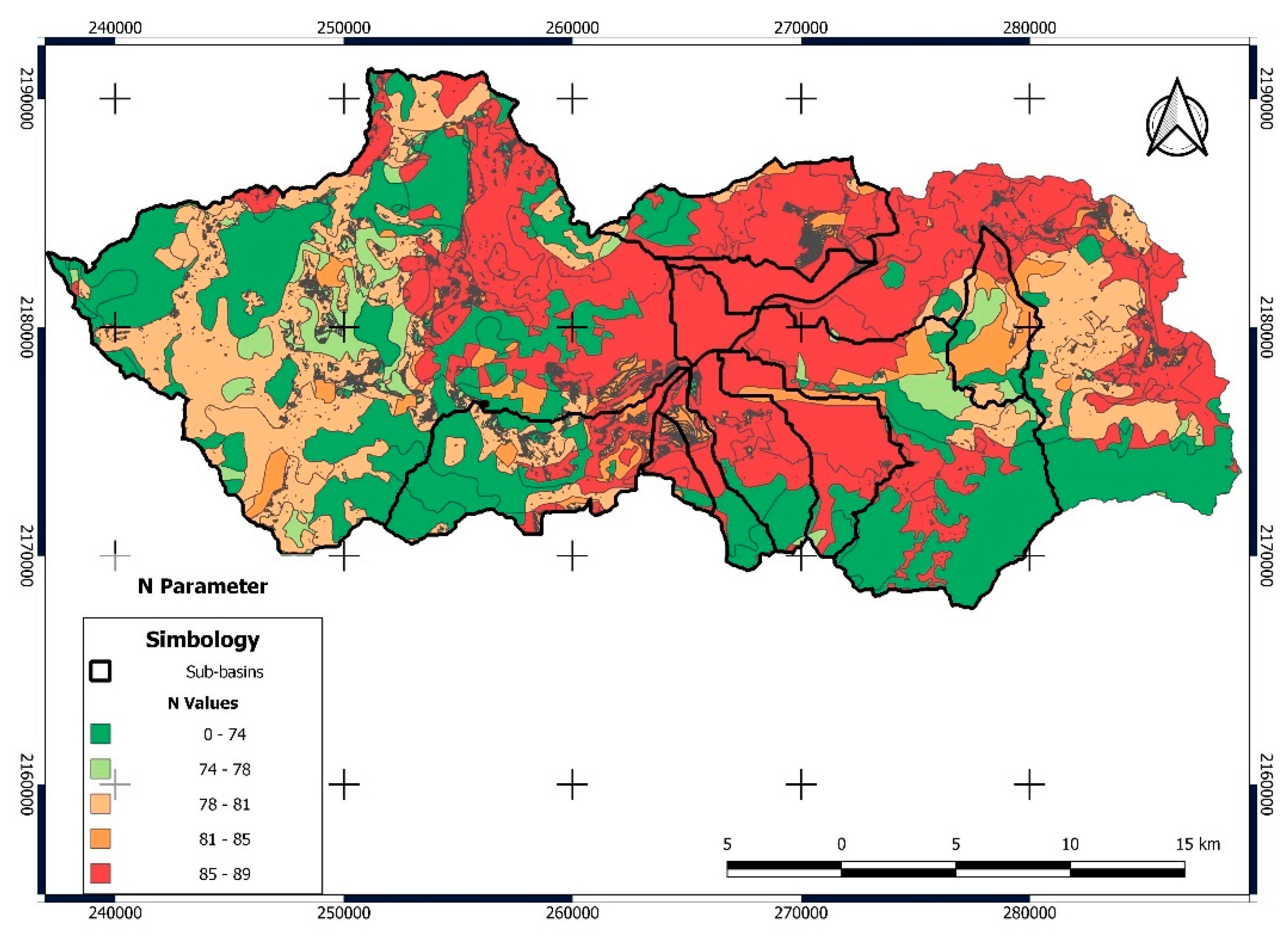
3.3. SCS-CN
3.4. Determination of Surface Runoff for All Subbasins
4. Discussion
5. Conclusions
Author Contributions
Funding
Data Availability Statement
Acknowledgments
Conflicts of Interest
Appendix A


References
- Beneyto, C.; Aranda, J.Á.; Benito, G.; Francés, F. New Approach to Estimate Extreme Flooding Using Continuous Synthetic Simulation Supported by Regional Precipitation and Non-Systematic Flood Data. Water 2020, 12, 3174. [Google Scholar] [CrossRef]
- Abreu, M.C.; Cecílio, R.A.; Pruski, F.F.; dos Santos, G.R.; de Almeida, L.T.; Zanetti, S.S. Criteria for Choosing Probability Distributions in Studies of Extreme Precipitation Events. Rev. Bras. Meteorol. 2018, 33, 601–613. [Google Scholar] [CrossRef]
- Segura-Beltrán, F.; Sanchis-Ibor, C.; Morales-Hernández, M.; González-Sanchis, M.; Bussi, G.; Ortiz, E. Using Post-Flood Surveys and Geomorphologic Mapping to Evaluate Hydrological and Hydraulic Models: The Flash Flood of the Girona River (Spain) in 2007. J. Hydrol. 2016, 541, 310–329. [Google Scholar] [CrossRef]
- Kastridis, A.; Theodosiou, G.; Fotiadis, G. Investigation of Flood Management and Mitigation Measures in Ungauged Natura Protected Watersheds. Hydrology 2021, 8, 170. [Google Scholar] [CrossRef]
- Coronado-Hernández, Ó.E.; Merlano-Sabalza, E.; Díaz-Vergara, Z.; Coronado-Hernández, J.R. Selection of Hydrological Probability Distributions for Extreme Rainfall Events in the Regions of Colombia. Water 2020, 12, 1397. [Google Scholar] [CrossRef]
- Flowers-Cano, R.S.; Ortiz-Gómez, R. Comparison of Four Methods to Select the Best Probability Distribution for Frequency Analysis of Annual Maximum Precipitation Using Monte Carlo Simulations. Theor. Appl. Climatol. 2021, 145, 1177–1192. [Google Scholar] [CrossRef]
- Moon, Y.-I.; Lall, U. Kernel Quantite Function Estimator for Flood Frequency Analysis. Water Resour. Res. 1994, 30, 3095–3103. [Google Scholar] [CrossRef]
- Petroselli, A.; De Luca, D.L.; Młyński, D.; Wałęga, A. Modelling Annual Maximum Daily Rainfall with the STORAGE (STOchastic RAinfall GEnerator) Model. Hydrol. Res. 2022, 53, 547–561. [Google Scholar] [CrossRef]
- Ciupak, M.; Ozga-Zieliński, B.; Tokarczyk, T.; Adamowski, J. A Probabilistic Model for Maximum Rainfall Frequency Analysis. Water 2021, 13, 2688. [Google Scholar] [CrossRef]
- Tarpanelli, A.; Franchini, M.; Brocca, L.; Camici, S.; Melone, F.; Moramarco, T. A Simple Approach for Stochastic Generation of Spatial Rainfall Patterns. J. Hydrol. 2012, 472–473, 63–76. [Google Scholar] [CrossRef]
- Alodah, A.; Seidou, O. Assessment of Climate Change Impacts on Extreme High and Low Flows: An Improved Bottom-Up Approach. Water 2019, 11, 1236. [Google Scholar] [CrossRef]
- Lele, S.; Keim, J.L. Weighted Distributions and Estimation of Resource Selection Probability Functions. Ecology 2006, 87, 3021–3028. [Google Scholar] [CrossRef] [PubMed]
- Venkata Rao, G.; Venkata Reddy, K.; Srinivasan, R.; Sridhar, V.; Umamahesh, N.V.; Pratap, D. Spatio-Temporal Analysis of Rainfall Extremes in the Flood-Prone Nagavali and Vamsadhara Basins in Eastern India. Weather Clim. Extrem. 2020, 29, 100265. [Google Scholar] [CrossRef]
- Dasallas, L.; An, H.; Lee, S. Developing an Integrated Multiscale Rainfall-Runoff and Inundation Model: Application to an Extreme Rainfall Event in Marikina-Pasig River Basin, Philippines. J. Hydrol. Reg. Stud. 2022, 39, 100995. [Google Scholar] [CrossRef]
- Gabriel, K.R.; Neumann, J. A Markov Chain Model for Daily Rainfall Occurrence at Tel Aviv. Q. J. R. Meteorol. Soc. 1962, 88, 90–95. [Google Scholar] [CrossRef]
- Hernández-Bedolla, J.; Solera, A.; Paredes-Arquiola, J.; Sanchez-Quispe, S.T.; Domínguez-Sánchez, C. A Continuous Multisite Multivariate Generator for Daily Temperature Conditioned by Precipitation Occurrence. Water 2022, 14, 3494. [Google Scholar] [CrossRef]
- Hayhoe, H.N. Improvements of Stochastic Weather Data Generators for Diverse Climates. Clim. Res. 2000, 14, 75–87. [Google Scholar] [CrossRef]
- Richardson, C.W.; Wright, D.A.; Nofziger, D.L.; Hornsby, A.G. WGEN: A Model for Generating Daily Weather Variables; U.S. Department of Agriculture: Washington, DC, USA, 1984.
- Marcello, D.; Gianni, B.; Ephrem, H.; Simone, B.; Roberto, C.; Bettina, B. CLIMA: A Weather Generator Framework. In Proceedings of the 18th World IMACS/MODSIM Congress, Cairns, Australia, 13–17 July 2009. [Google Scholar]
- Stöckle, C.O.; Nelson, R.; Donatelli, M.; Castellvì, F. ClimGen: A Flexible Weather Generation Program. In Proceedings of the 2nd International Symposium Modelling Cropping Systems, Florence, Italy, 16–18 July 2001; pp. 16–18. [Google Scholar]
- Semenov, M.A.; Barrow, E.M. User´s guide: LARS-WG A Stochastic Weather Generator for Use in Climate Impact Studies LARS-WG: Stochastic Weather Generator Contents; Rothamsted: Harpended, Hertfordshire, UK, 2002. [Google Scholar]
- Chen, J.; Brissette, F.P.; Leconte, R. WeaGETS—A Matlab-Based Daily Scale Weather Generator for Generating Precipitation and Temperature. Procedia Environ. Sci. 2012, 13, 2222–2235. [Google Scholar] [CrossRef]
- Mehrotra, R.; Li, J.; Westra, S.; Sharma, A. A Programming Tool to Generate Multi-Site Daily Rainfall Using a Two-Stage Semi Parametric Model. Environ. Model. Softw. 2015, 63, 230–239. [Google Scholar] [CrossRef]
- Carter, T.; Posch, M.; Tuomenvirta, H. SILMUSCEN and CLIGEN User’s Guide: Guidelines for the Construction of Climatic Scenarios and Use of a Stochastic Weather Generator in the Finnish; Academy of Finland: Helsinki, Finland, 1995. [Google Scholar]
- Richardson, C.W. Stochastic Simulation of Daily Precipitation, Temperature, and Solar Radiation. Water Resour. Res. 1981, 17, 182–190. [Google Scholar] [CrossRef]
- Rayner, D.; Achberger, C.; Chen, D. A Multi-State Weather Generator for Daily Precipitation for the Torne River Basin, Northern Sweden/Western Finland. Adv. Clim. Change Res. 2016, 7, 70–81. [Google Scholar] [CrossRef]
- Humphrey, G.B.; Gibbs, M.S.; Dandy, G.C.; Maier, H.R. A Hybrid Approach to Monthly Streamflow Forecasting: Integrating Hydrological Model Outputs into a Bayesian Artificial Neural Network. J. Hydrol. 2016, 540, 623–640. [Google Scholar] [CrossRef]
- Portoghese, I.; Bruno, E.; Guyennon, N.; Iacobellis, V. Stochastic Bias-Correction of Daily Rainfall Scenarios for Hydrological Applications. Nat. Hazards Earth Syst. Sci. 2011, 11, 2497–2509. [Google Scholar] [CrossRef]
- Wang, L.; Onof, C. Analysis of sub-daily rainfall sequences based upon a semi-deterministic multiplicative cascade method. In Proceedings of the International Workshop on Advances in Statistical Hydrology, Taormina, Italy, 23–25 May 2010; pp. 1–9. [Google Scholar]
- Vandenberghe, S.; Verhoest, N.E.C.; Buyse, E.; De Baets, B. A Stochastic Design Rainfall Generator Based on Copulas and Mass Curves. Hydrol. Earth Syst. Sci. 2010, 14, 2429–2442. [Google Scholar] [CrossRef]
- Katz, R.W.; Parlange, M.B. Generalizations of Chain-Dependent Processes: Application to Hourly Precipitation. Water Resour. Res. 1995, 31, 1331–1341. [Google Scholar] [CrossRef]
- Koch, E.; Naveau, P. A Frailty-Contagion Model for Multi-Site Hourly Precipitation Driven by Atmospheric Covariates. Adv. Water Resour. 2015, 78, 145–154. [Google Scholar] [CrossRef]
- Ailliot, P.; Allard, D.; Monbet, V.; Naveau, P. Stochastic Weather Generators: An Overview of Weather Type Models. J. Société Française Stat. Rev. Stat. Appliquée 2015, 156, 101–113. [Google Scholar]
- Wilks, D.S. Multisite Generalization of a Daily Stochastic Precipitation Generation Model. J. Hydrol. 1998, 210, 178–191. [Google Scholar] [CrossRef]
- Anderson, R.L. Distribution of the Serial Correlation Coefficient. Ann. Math. Stat. 1942, 13, 1–13. [Google Scholar] [CrossRef]
- Moors, D.S.; Stubblebine, J.B. Chi-Square Tests for multivariate normality with application to common stock prices. Commun. Stat.-Theory Methods 1981, 10, 713–738. [Google Scholar]
- Hu, S. Akaike Information Criterion Statistics. Math. Comput. Simul. 1987, 29, 452. [Google Scholar] [CrossRef]
- Lima, A.O.; Lyra, G.B.; Abreu, M.C.; Oliveira-Júnior, J.F.; Zeri, M.; Cunha-Zeri, G. Extreme Rainfall Events over Rio de Janeiro State, Brazil: Characterization Using Probability Distribution Functions and Clustering Analysis. Atmos. Res. 2021, 247, 105221. [Google Scholar] [CrossRef]
- Simolo, C.; Brunetti, M.; Maugeri, M.; Nanni, T. Improving Estimation of Missing Values in Daily Precipitation Series by a Probability Density Function-Preserving Approach. Int. J. Climatol. 2010, 30. [Google Scholar] [CrossRef]
- Li, C.; Singh, V.P.; Mishra, A.K. Simulation of the Entire Range of Daily Precipitation Using a Hybrid Probability Distribution. Water Resour. Res. 2012, 48, 3521. [Google Scholar] [CrossRef]
- Shin, Y.; Park, J.S. Modeling Climate Extremes Using the Four-Parameter Kappa Distribution for r-Largest Order Statistics. Weather Clim. Extrem. 2023, 39, 100533. [Google Scholar] [CrossRef]
- Alahmadi, F.S.; Rahman, N.A. Climate Change Impacts on Extreme Rainfall Frequency Prediction. J. Water Clim. Change 2020, 11, 935–943. [Google Scholar] [CrossRef]
- Nwaogazie, I.L.; Sam, M.G.; Enciso, R.Z.; Gonsalves, E. Probability and Non-Probability Rainfall Intensity-Duration-Frequency Modeling for Port-Harcourt Metropolis, Nigeria. Int. J. Hydrol. 2019, 3, 66–75. [Google Scholar] [CrossRef]
- Bajirao, T.S. Comparative Performance of Different Probability Distribution Functions for Maximum Rainfall Estimation at Different Time Scales. Arab. J. Geosci. 2021, 14, 2138. [Google Scholar] [CrossRef]
- Devkota, S.; Shakya, N.M.; Sudmeier-Rieux, K.; Jaboyedoff, M.; Van Westen, C.J.; Mcadoo, B.G.; Adhikari, A. Development of Monsoonal Rainfall Intensity-Duration-Frequency (IDF) Relationship and Empirical Model for Data-Scarce Situations: The Case of the Central-Western Hills (Panchase Region) of Nepal. Hydrology 2018, 5, 27. [Google Scholar] [CrossRef]
- Pizarro, R.; Valdés, R.; García-Chevesich, P.; Vallejos, C.; Sangüesa, C.; Morales, C.; Balocchi, F.; Abarza, A.; Fuentes, R. Latitudinal Analysis of Rainfall Intensity and Mean Annual Precipitation in Chile. Chil. J. Agric. Res. 2012, 72, 252–261. [Google Scholar] [CrossRef]
- Villón-Béjar, M. HidroEsta, Software for Hydrological Calculations. Rev. Tecnol. En Marcha 2016, 29, 95–108. [Google Scholar] [CrossRef]
- Villón Béjar, M. HidroEsta, Software Para Cálculos Hidrológicos. Tecnol. En Marcha 2005, 18, 67. [Google Scholar]
- Villón Béjar, M. HidroEsta, Software Para Cálculos Hidrológicos y Estadísticos Aplicados a La Hidrología. Rev. Digit. Matemática Educ. E Internet 2014, 12, 1–8. [Google Scholar] [CrossRef]
- García Castro, E.G. Estimación de caudales máximos en el rio Chira, utilizando métodos estadisticos de Gumbel y de Pearson tipo III; Universidad Nacional de Piura: Castilla, Piura, Peru, 2023. [Google Scholar]
- Mendoza, R.; Zavala, J.; Villa, S. Revisión de Gastos de Diseño de La Presa Huites Mediante Relaciones Lluvia-Escurrimiento. Ing. Hidráulica Y Ambient. 2014, XXXV, 77–89. [Google Scholar]
- Yu, B. Theoretical Justification of SCS Method for Runoff Estimation. J. Irrig. Drain. Eng. 1998, 124, 306–310. [Google Scholar] [CrossRef]
- Hawkins, R.H.; Hjelmfelt, A.T.; Zevenbergen, A.W. Runoff Probability, Storm Depth, and Curve Numbers. J. Irrig. Drain. Eng. 1985, 111, 330–340. [Google Scholar] [CrossRef]
- Yu, B. Validation of SCS Method for Runoff Estimation. J. Hydrol. Eng. 2012, 17, 1158–1163. [Google Scholar] [CrossRef]
- Boughton, W.C. A Review of the USDA SCS Curve Number Method. Aust. J. Soil Res. 1989, 27, 511–523. [Google Scholar] [CrossRef]
- Hooshyar, M.; Wang, D. An Analytical Solution of Richards’ Equation Providing the Physical Basis of SCS Curve Number Method and Its Proportionality Relationship. Water Resour. Res. 2016, 52, 6611–6620. [Google Scholar] [CrossRef]
- Kirkby, M.; Cerdà, A. Following the Curve? Reviewing the Physical Basis of the SCS Curve Number Method for Estimating Storm Runoff. Hydrol. Process. 2021, 35, e14404. [Google Scholar] [CrossRef]
- Stathi, E.; Kastridis, A.; Myronidis, D. Analysis of Hydrometeorological Characteristics and Water Demand in Semi-Arid Mediterranean Catchments under Water Deficit Conditions. Climate 2023, 11, 137. [Google Scholar] [CrossRef]
- Verma, S.; Verma, R.K.; Mishra, S.K.; Singh, A.; Jayaraj, G.K. A Revisit of NRCS-CN Inspired Models Coupled with RS and GIS for Runoff Estimation. Hydrol. Sci. J. 2017, 62, 1891–1930. [Google Scholar] [CrossRef]
- Satheeshkumar, S.; Venkateswaran, S.; Kannan, R. Rainfall–Runoff Estimation Using SCS–CN and GIS Approach in the Pappiredipatti Watershed of the Vaniyar Sub Basin, South India. Model. Earth Syst. Environ. 2017, 3, 24. [Google Scholar] [CrossRef]
- Halwatura, D.; Najim, M.M.M. Application of the HEC-HMS Model for Runoff Simulation in a Tropical Catchment. Environ. Model. Softw. 2013, 46, 155–162. [Google Scholar] [CrossRef]
- Gimeno, L.; Sorí, R.; Vázquez, M.; Stojanovic, M.; Algarra, I.; Eiras-Barca, J.; Gimeno-Sotelo, L.; Nieto, R. Extreme Precipitation Events. Wiley Interdiscip. Rev. Water 2022, 9, e1611. [Google Scholar] [CrossRef]
- Chen, X.; Hossain, F. Understanding Future Safety of DAMs in a Changing Climate. Bull. Am. Meteorol. Soc. 2019, 100, 1395–1404. [Google Scholar] [CrossRef]
- Yin, C.; Wang, J.; Yu, X.; Li, Y.; Yan, D.; Jian, S. Definition of Extreme Rainfall Events and Design of Rainfall Based on the Copula Function. Water Resour. Manag. 2022, 36, 3759–3778. [Google Scholar] [CrossRef]
- Zhu, B.; Chen, J.; Chen, H. Performance of Multiple Probability Distributions in Generating Daily Precipitation for the Simulation of Hydrological Extremes. Stoch. Environ. Res. Risk Assess. 2019, 33, 1581–1592. [Google Scholar] [CrossRef]
- Chen, J.; Brissette, F.P.; Zielinski, P.A. Constraining Frequency Distributions with the Probable Maximum Precipitation for the Stochastic Generation of Realistic Extreme Events. J. Extrem. Events 2015, 2, 1550009. [Google Scholar] [CrossRef]
- Chen, J.; Brissette, F.P.; Chaumont, D.; Braun, M. Performance and Uncertainty Evaluation of Empirical Downscaling Methods in Quantifying the Climate Change Impacts on Hydrology over Two North American River Basins. J. Hydrol. 2013, 479, 200–214. [Google Scholar] [CrossRef]
- Chen, J.; Brissette, F.P.; Zhang, X.J. Hydrological Modeling Using a Multisite Stochastic Weather Generator. J. Hydrol. Eng. 2016, 21, 04015060. [Google Scholar] [CrossRef]
- Chen, J.; Brissette, F.P.; Leconte, R. Downscaling of Weather Generator Parameters to Quantify Hydrological Impacts of Climate Change. Clim. Res. 2012, 51, 185–200. [Google Scholar] [CrossRef]
- Hernández-Bedolla, J. Análisis de Datos Climáticos Como Predictor Para La Gestión Anticipada de Sequias. Ph.D. Thesis, Universidad Politecnica de Valencia, Valence, Spain, 2022. [Google Scholar]
- Sparks, N.J.; Hardwick, S.R.; Schmid, M.; Toumi, R. IMAGE: A Multivariate Multi-Site Stochastic Weather Generator for European Weather and Climate. Stoch. Environ. Res. Risk Assess. 2018, 32, 771–784. [Google Scholar] [CrossRef]
- Chen, J.; Brissette, F.P.; Leconte, R. A Daily Stochastic Weather Generator for Preserving Low-Frequency of Climate Variability. J. Hydrol. 2010, 388, 480–490. [Google Scholar] [CrossRef]
- Gu, L.; Chen, J.; Xu, C.; Kim, J.; Chen, H.; Xia, J.; Zhang, L. The Contribution of Internal Climate Variability to Climate Change Impacts on Droughts. Sci. Total Environ. 2019, 684, 229–246. [Google Scholar] [CrossRef]
- Li, Z.; Brissette, F.; Chen, J. Finding the Most Appropriate Precipitation Probability Distribution for Stochastic Weather Generation and Hydrological Modelling in Nordic Watersheds. Hydrol. Process. 2013, 27, 3718–3729. [Google Scholar] [CrossRef]
- Rawat, K.S.; Singh, S.K. Estimation of Surface Runoff from Semi-Arid Ungauged Agricultural Watershed Using SCS-CN Method and Earth Observation Data Sets. Water Conserv. Sci. Eng. 2017, 1, 233–247. [Google Scholar] [CrossRef]
- Ouaba, M.; Saidi, M.E.; Alam, M.J. Bin Flood Modeling through Remote Sensing Datasets Such as LPRM Soil Moisture and GPM-IMERG Precipitation: A Case Study of Ungauged Basins across Morocco. Earth Sci. Inform. 2023, 16, 653–674. [Google Scholar] [CrossRef]
- Meresa, H. Modelling of River Flow in Ungauged Catchment Using Remote Sensing Data: Application of the Empirical (SCS-CN), Artificial Neural Network (ANN) and Hydrological Model (HEC-HMS). Model Earth Syst. Environ. 2019, 5, 257–273. [Google Scholar] [CrossRef]
- Topçuoğlu, M.E.; Karagüzel, R.; Doğan, A. Comparison of the SCS-CN and Hydrograph Separation Method for Runoff Estimation in an Ungauged Basin: The Izmit Basin, Turke. Int. J. Econ. Environ. Geol. 2022, 12, 22–31. [Google Scholar] [CrossRef]
- Ningaraju, H.J.; Kumar, S.B.G.; Surendra, H.J. Estimation of Runoff Using SCS-CN and GIS Method in Ungauged Watershed: A Case Study of Kharadya Mill Watershed, India. Int. J. Adv. Eng. Res. Sci. 2016, 3, 36–42. [Google Scholar]
- Hashim, H.Q.; Sayl, K.N. Incorporating GIS Technique and SCS-CN Approach for Runoff Estimation in the Ungauged Watershed: A Case Study West Desert of Iraq. Iraqi J. Civ. Eng. 2022, 14, 1–6. [Google Scholar] [CrossRef]
- Nageswara Rao, K. Analysis of Surface Runoff Potential in Ungauged Basin Using Basin Parameters and SCS-CN Method. Appl. Water Sci. 2020, 10, 47. [Google Scholar] [CrossRef]
- Jeon, J.H.; Lim, K.J.; Engel, B.A. Regional Calibration of SCS-CN L-THIA Model: Application for Ungauged Basins. Water 2014, 6, 1339–1359. [Google Scholar] [CrossRef]
- Moid Mohammed, A.; Lakshmi Thatiparthi, V.; Rao Pyla, K.; Maryada, A. Estimation of Surface Runoff in an Ungauged Basin Using SCS-CN Method, A Case Study of Manair River Basin in Telangana, India. Appl. Ecol. Environ. Sci. 2020, 8, 340–350. [Google Scholar] [CrossRef]
- Faouzi, E.; Arioua, A.; Hssaisoune, M.; Boudhar, A.; Elaloui, A.; Karaoui, I. Sensitivity Analysis of CN Using SCS-CN Approach, Rain Gauges and TRMM Satellite Data Assessment into HEC-HMS Hydrological Model in the Upper Basin of Oum Er Rbia, Morocco. Model Earth Syst. Environ. 2022, 8, 4707–4729. [Google Scholar] [CrossRef]
- Juma, B.; Olang, L.O.; Hassan, M.A.; Mulligan, J.; Shiundu, P.M. Simulation of Flood Peak Discharges and Volumes for Flood Risk Management in the Ungauged Urban Informal Settlement of Kibera, Kenya. Phys. Chem. Earth 2022, 128, 103236. [Google Scholar] [CrossRef]
- Bharali, B.; Misra, U.K. Numerical Approach for Channel Flood Routing in an Ungauged Basin: A Case Study in Kulsi River Basin, India. Water Conserv. Sci. Eng. 2022, 7, 389–404. [Google Scholar] [CrossRef]
- Ouaba, M.; El Khalki, E.M.; Saidi, M.E.; Alam, M.J. Bin Estimation of Flood Discharge in Ungauged Basin Using GPM-IMERG Satellite-Based Precipitation Dataset in a Moroccan Arid Zone. Earth Syst. Environ. 2022, 6, 541–556. [Google Scholar] [CrossRef]
- Forootan, E. GIS-Based Slope-Adjusted Curve Number Methods for Runoff Estimation. Environ. Monit. Assess. 2023, 195, 489. [Google Scholar] [CrossRef]


| Station | Latitude (°) | Longitude (°) | Elevation (msnm) | Years | Total Annual Precipitation (mm/year) | Pmax * (mm/year) |
|---|---|---|---|---|---|---|
| 16022 | 19.625 | −101.281 | 2096 | 1980−2009 | 811.8 | 78 |
| 16247 | 19.675 | 101.392 | 2097 | 1980−2009 | 700.7 | 75.3 |
| 16055 | 19.652 | −101.151 | 2180 | 1980−2009 | 1092.25 | 97 |
| 16081 | 16.289 | −101.176 | 1913 | 1980−2009 | 772.21 | 80.1 |
| Statistical/Station | 16055 | 16081 | 16022 | 16247 |
|---|---|---|---|---|
| Mean | −0.0084 | −0.0035 | 0.080 | −0.078 |
| Standard deviation | 1.0431 | 1.0843 | 1.3315 | 1.0895 |
| Skewness coefficient | −0.1212 | 0.3246 | 0.5622 | −0.0939 |
| Lag-one autocorrelation | 0.0239 | 0.0420 | 0.0461 | −0.0581 |
| AIC | −2145 | −1995 | −4733 | −2652 |
| Function/Station | 16055 | 16081 | 16022 | 16247 |
|---|---|---|---|---|
| Normal | 0.1977 | 0.1138 | 0.1932 | 0.1193 |
| Log-Normal 3P | 0.1064 | 0.0592 | 0.0696 * | 0.1044 |
| Log-Normal 2P | 0.1187 | 0.0618 | 0.1164 | 0.0907 * |
| Gamma 2P | 0.1427 | 0.0798 | 0.1433 | 0.1025 |
| Gamma 3P | N/A | 0.05595 | N/A | 0.09575 |
| Log Pearson III | 0.09761 | 0.0511 | N/A | N/A |
| Gumbel | 0.1347 | 0.045 * | 0.1478 | 0.0994 |
| Log Gumbel | 0.0871 * | 0.0596 | 0.079 | 0.0924 |
| Model | TR | 16022 | 16247 | 16055 | 16081 |
|---|---|---|---|---|---|
| MASVC | 2 | 34.99 | 40.05 | 47.73 | 31.65 |
| 5 | 43.78 | 50.47 | 59.49 | 47.45 | |
| 10 | 58.26 | 64.33 | 71.87 | 59.36 | |
| 20 | 69.58 | 79.31 | 84.41 | 72.07 | |
| 50 | 87.33 | 99.25 | 101.34 | 91.33 | |
| 100 | 102.25 | 112.2 | 116.51 | 105.23 | |
| 2 | 40.66 | 41.01 | 31.27 | 42.7 | |
| 5 | 52.61 | 56.2 | 43.61 | 53.75 | |
| 10 | 61.63 | 66.27 | 54.35 | 61.07 | |
| 20 | 71.03 | 75.93 | 67.13 | 68.09 | |
| 50 | 84.27 | 88.49 | 88.23 | 77.18 | |
| 100 | 95.02 | 98 | 108.28 | 83.99 |
| Subbasin * | Area (km2) | Height Difference (m) | Length of the Main Channel (m) | Slope (%) | Concentration Time (h) | CN |
|---|---|---|---|---|---|---|
| 1 | 308.32 | 898 | 30,833.01 | 2.41 | 3.62 | 76.35 |
| 2 | 47.62 | 1132 | 16,106.46 | 5.72 | 1.56 | 78.36 |
| 4 | 24.3 | 459 | 11,451.81 | 5.32 | 1.49 | 84.47 |
| 5 | 26.67 | 561 | 12,862.88 | 4.58 | 1.58 | 83.14 |
| 6 | 86.79 | 416 | 21,086.86 | 1.13 | 3.13 | 77.03 |
| 8 | 18.85 | 230 | 9394.3 | 2.46 | 1.55 | 84.16 |
| 12 | 40.19 | 792 | 14,307.83 | 4.77 | 1.56 | 85.09 |
| 13 | 10.01 | 258 | 4614.52 | 5.14 | 0.65 | 86.87 |
| 14 | 6.11 | 220 | 4114.46 | 3.95 | 0.61 | 86.02 |
| 15 | 11.3 | 671 | 9878.71 | 3.67 | 1.08 | 84.67 |
| 16 | 10.71 | 1.93 | 453.54 | 0.43 | 0.29 | 87.21 |
| Model | * Subbasin/Tr | 2 | 5 | 10 | 20 | 50 | 100 |
|---|---|---|---|---|---|---|---|
| MASVC-SCS-CN | 1 | 9.68 | 35.01 | 88.48 | 166.82 | 298.97 | 394.90 |
| 2 | 0.32 | 1.49 | 9.86 | 20.72 | 44.11 | 68.85 | |
| 4 | 0.11 | 1.45 | 5.39 | 11.93 | 25.73 | 38.10 | |
| 5 | 1.45 | 6.11 | 13.08 | 22.26 | 36.62 | 53.63 | |
| 6 | 4.38 | 13.76 | 28.25 | 47.08 | 78.03 | 110.21 | |
| 8 | 0.11 | 1.17 | 25.30 | 30.72 | 38.93 | 44.85 | |
| 12 | 0.93 | 2.51 | 9.08 | 19.89 | 42.50 | 62.65 | |
| 13 | 0.05 | 0.47 | 2.86 | 7.39 | 17.72 | 27.20 | |
| 14 | 0.02 | 0.10 | 1.75 | 4.29 | 10.12 | 16.44 | |
| 15 | 0.01 | 0.12 | 1.93 | 4.64 | 10.78 | 17.52 | |
| 16 | 0.23 | 0.94 | 2.95 | 6.09 | 12.43 | 17.95 | |
| PDF-SCS-CN | 1 | 10.56 | 52.59 | 104.17 | 142.81 | 217.25 | 280.62 |
| 2 | 0.98 | 7.06 | 16.79 | 25.42 | 44.15 | 62.26 | |
| 4 | 0.91 | 4.24 | 5.08 | 7.64 | 17.92 | 23.30 | |
| 5 | 0.33 | 1.11 | 5.81 | 11.47 | 28.00 | 48.51 | |
| 6 | 2.21 | 3.06 | 13.73 | 25.48 | 59.66 | 101.38 | |
| 8 | 0.67 | 3.16 | 3.79 | 5.68 | 13.39 | 17.45 | |
| 12 | 1.40 | 6.67 | 7.99 | 12.02 | 28.33 | 36.87 | |
| 13 | 0.11 | 1.73 | 2.15 | 3.72 | 10.53 | 14.29 | |
| 14 | 0.10 | 0.90 | 2.74 | 4.70 | 8.98 | 13.24 | |
| 15 | 0.06 | 1.34 | 3.74 | 6.01 | 11.05 | 16.06 | |
| 16 | 0.60 | 2.29 | 2.61 | 3.91 | 8.65 | 11.06 |
Disclaimer/Publisher’s Note: The statements, opinions and data contained in all publications are solely those of the individual author(s) and contributor(s) and not of MDPI and/or the editor(s). MDPI and/or the editor(s) disclaim responsibility for any injury to people or property resulting from any ideas, methods, instructions or products referred to in the content. |
© 2023 by the authors. Licensee MDPI, Basel, Switzerland. This article is an open access article distributed under the terms and conditions of the Creative Commons Attribution (CC BY) license (https://creativecommons.org/licenses/by/4.0/).
Share and Cite
Hernández-Bedolla, J.; García-Romero, L.; Franco-Navarro, C.D.; Sánchez-Quispe, S.T.; Domínguez-Sánchez, C. Extreme Runoff Estimation for Ungauged Watersheds Using a New Multisite Multivariate Stochastic Model MASVC. Water 2023, 15, 2994. https://doi.org/10.3390/w15162994
Hernández-Bedolla J, García-Romero L, Franco-Navarro CD, Sánchez-Quispe ST, Domínguez-Sánchez C. Extreme Runoff Estimation for Ungauged Watersheds Using a New Multisite Multivariate Stochastic Model MASVC. Water. 2023; 15(16):2994. https://doi.org/10.3390/w15162994
Chicago/Turabian StyleHernández-Bedolla, Joel, Liliana García-Romero, Chrystopher Daly Franco-Navarro, Sonia Tatiana Sánchez-Quispe, and Constantino Domínguez-Sánchez. 2023. "Extreme Runoff Estimation for Ungauged Watersheds Using a New Multisite Multivariate Stochastic Model MASVC" Water 15, no. 16: 2994. https://doi.org/10.3390/w15162994