
Experimental and Computational Fluid Dynamic Study of Water Flow and Submerged Depth Effects on a Tidal Turbine Performance


Abstract
:1. Introduction
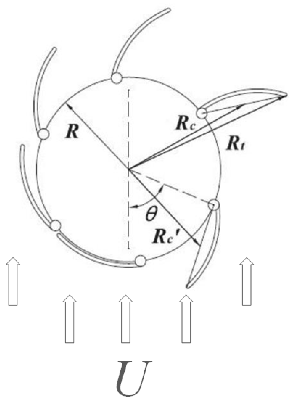
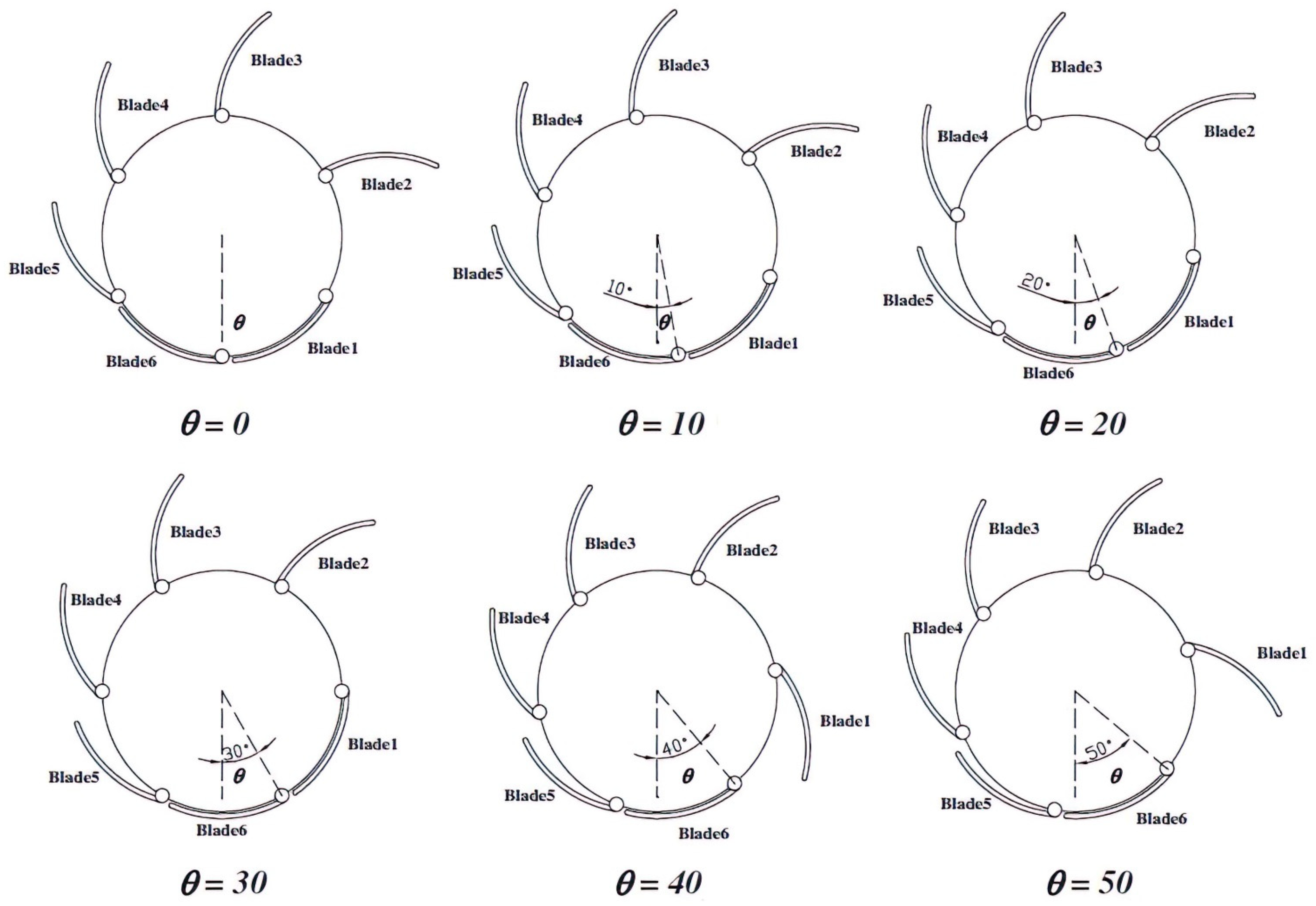
2. Methodology
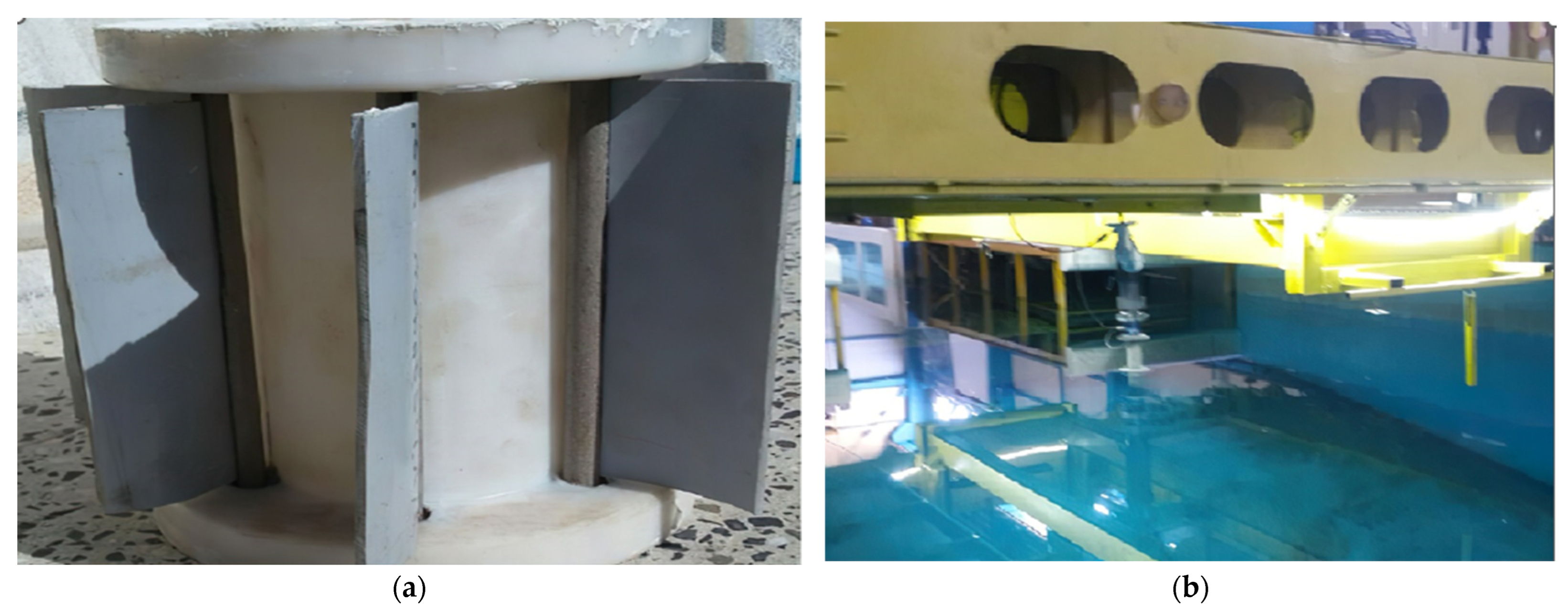
3. Setup
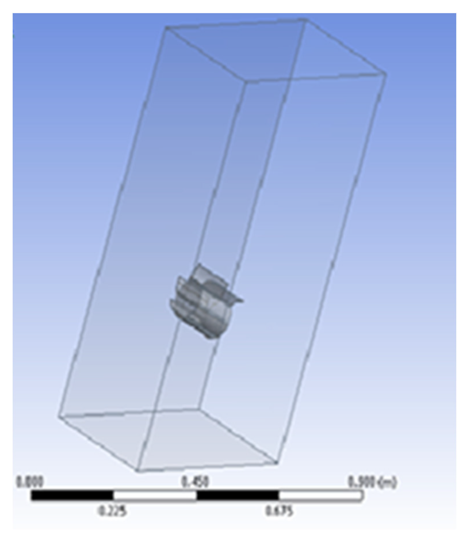
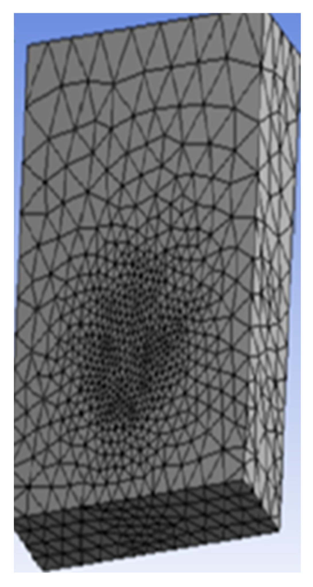
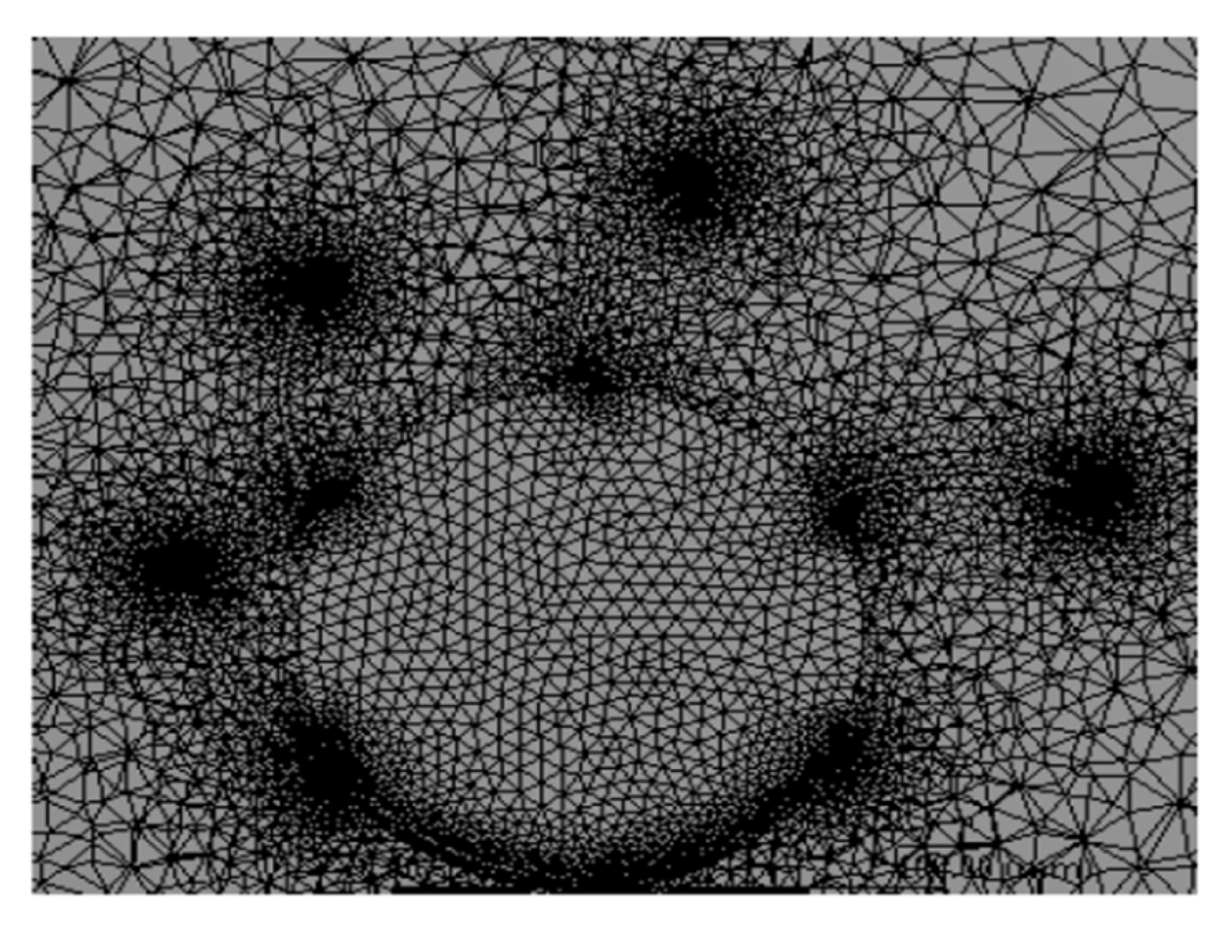
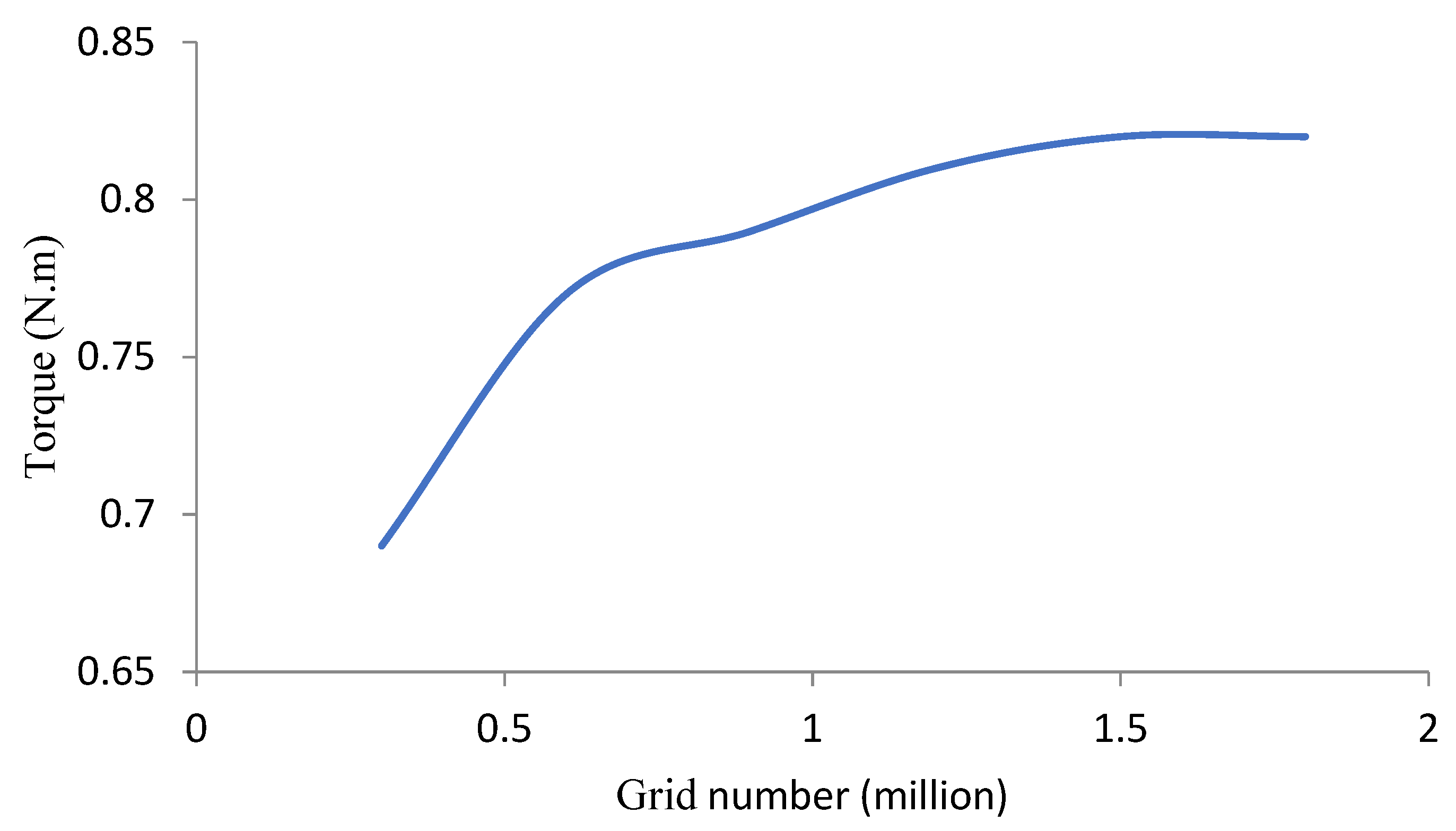
4. Numerical Setup
5. Results and Discussion
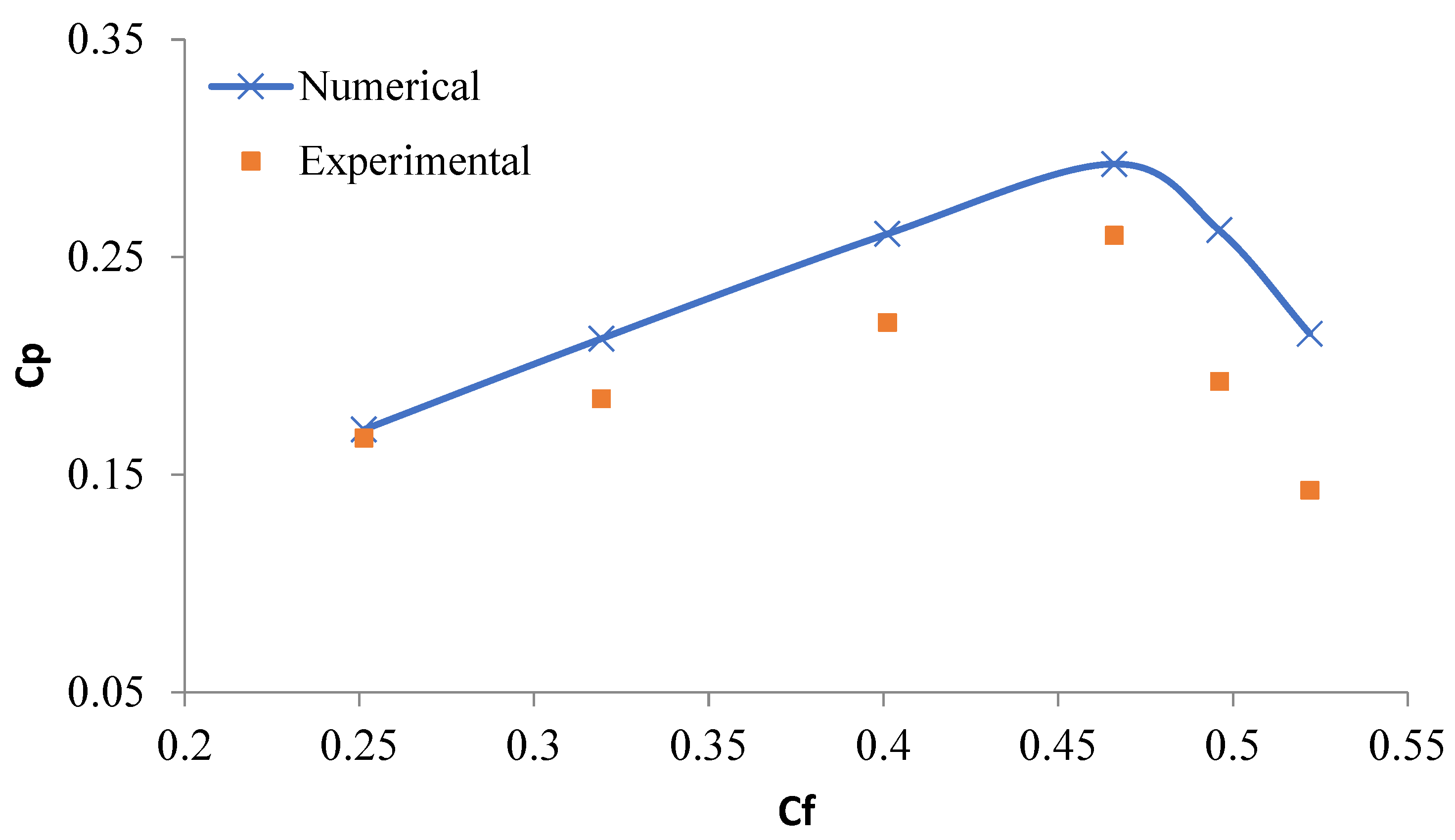
5.1. The Performance of a Stand-Alone Turbine
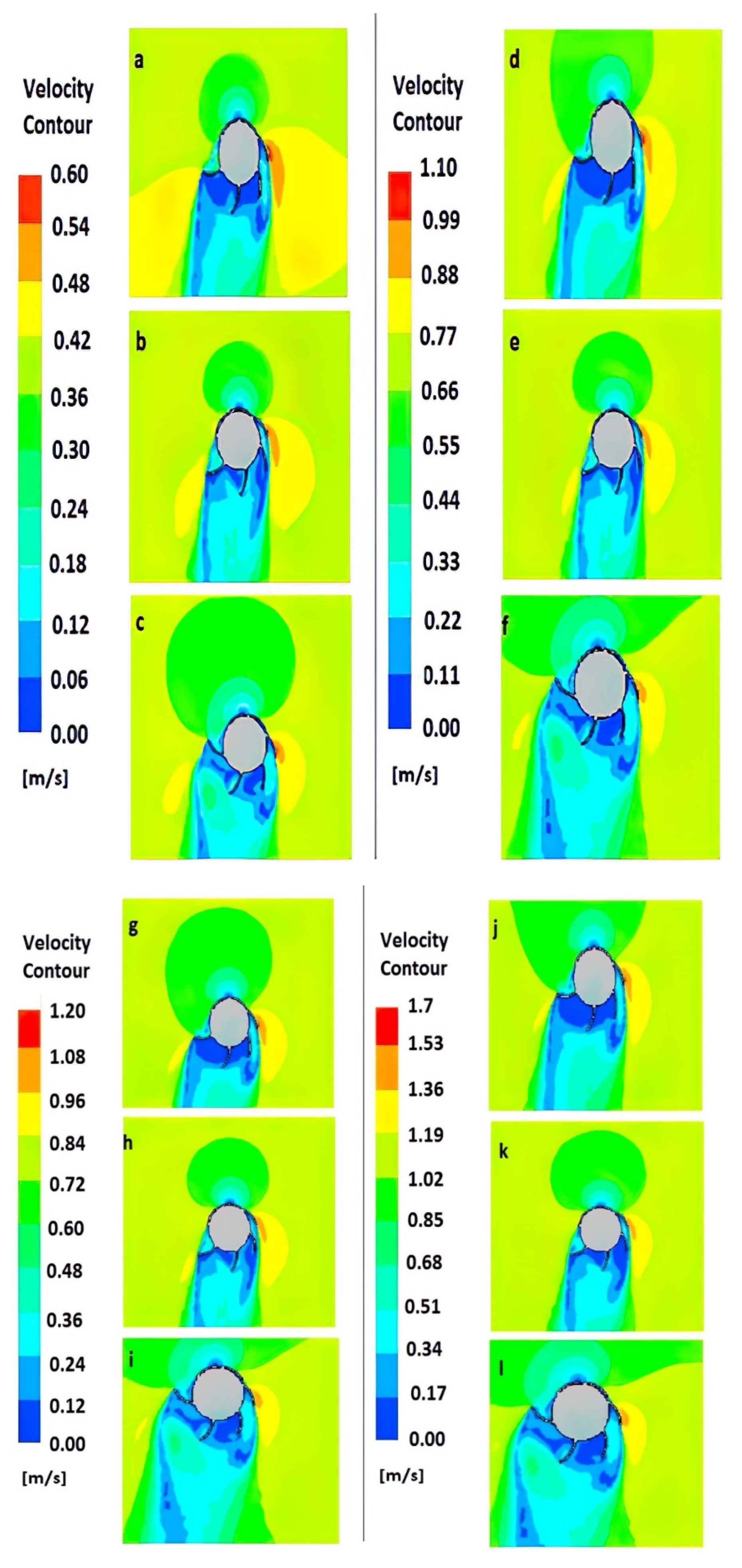
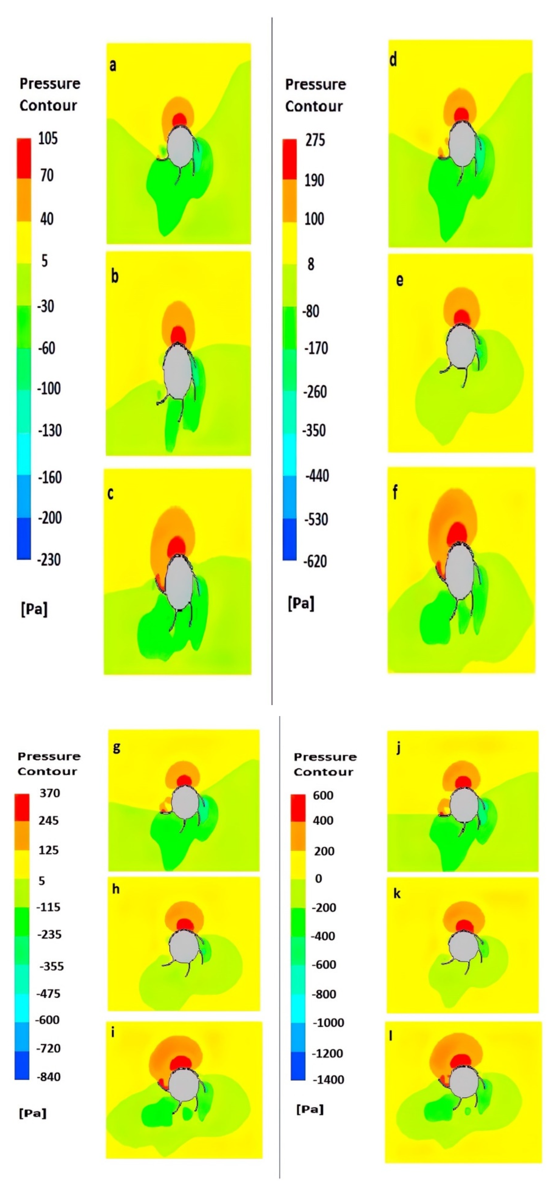
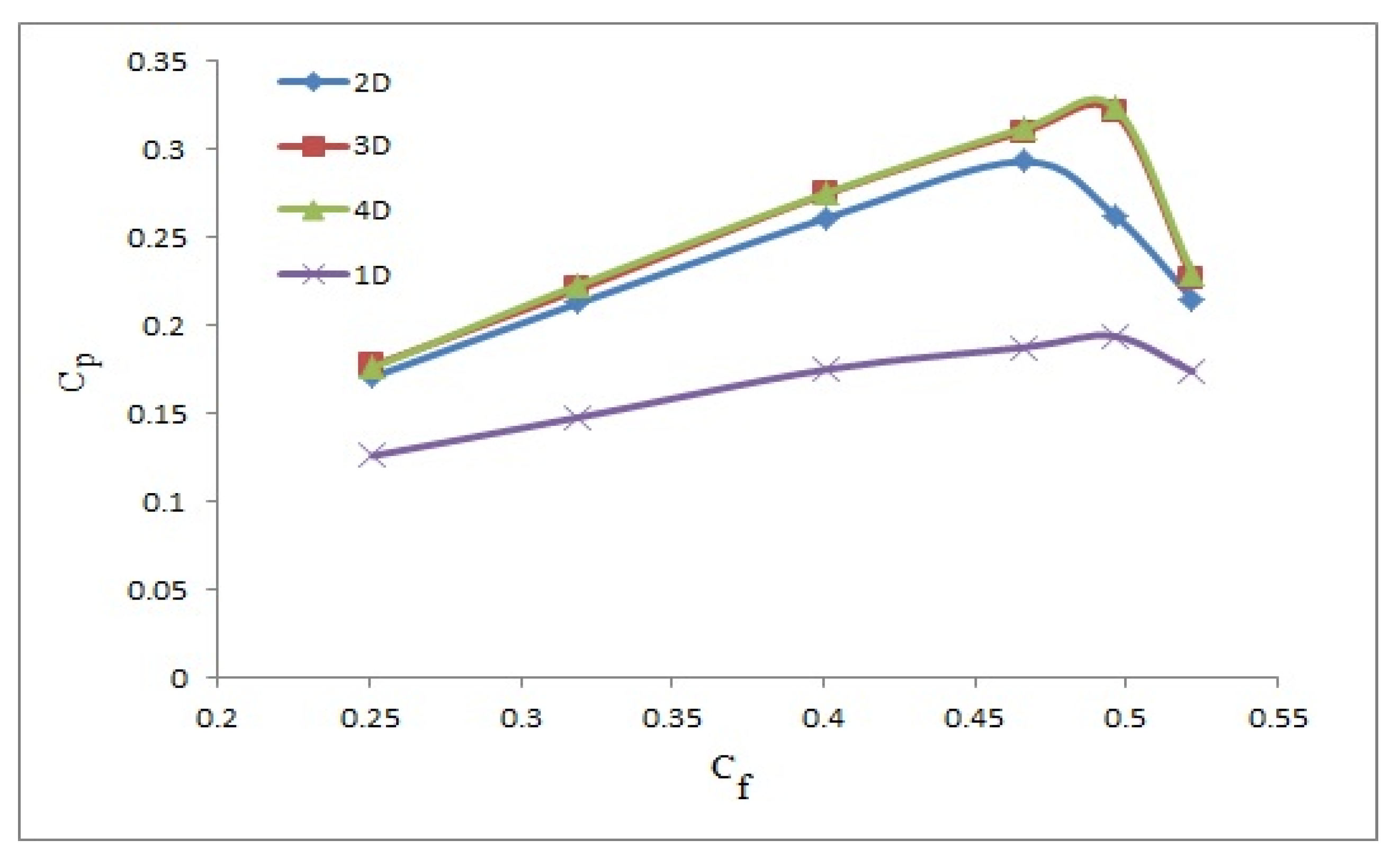
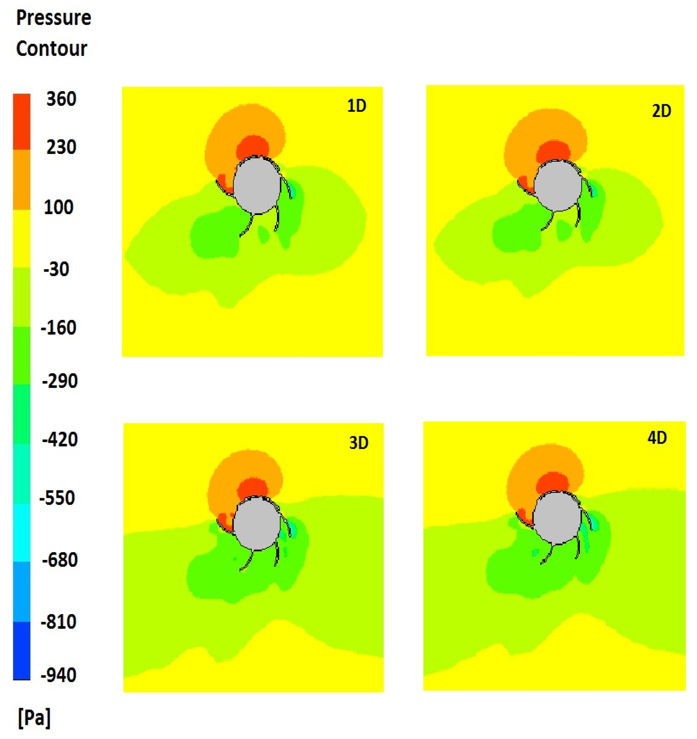
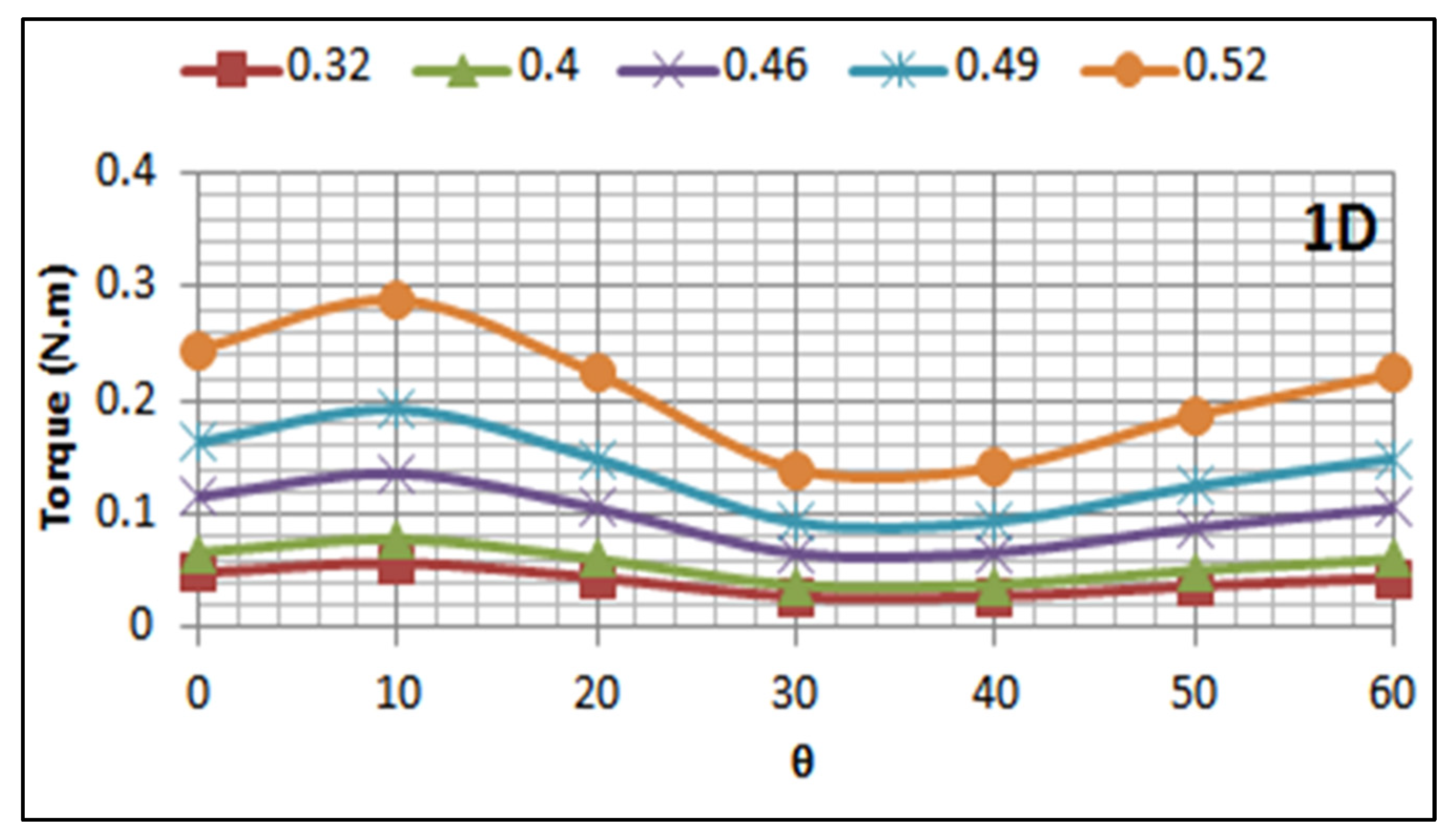
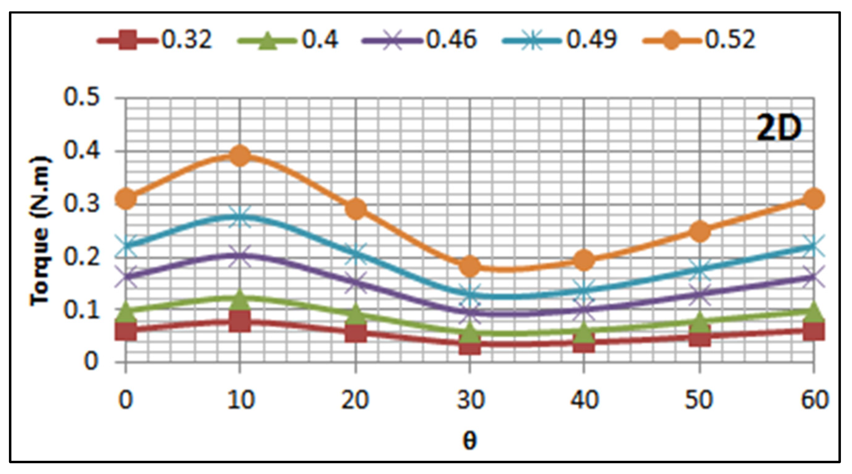
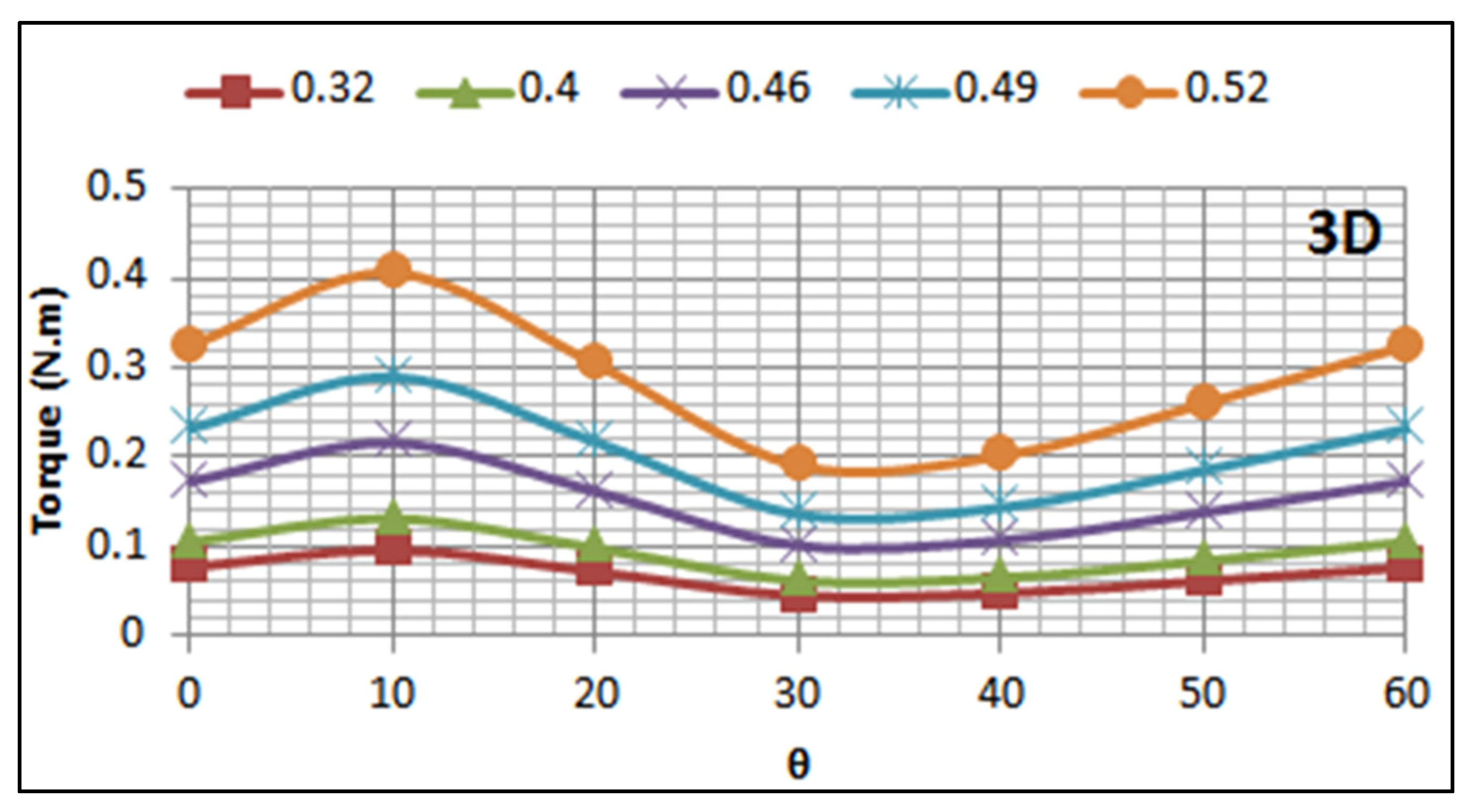
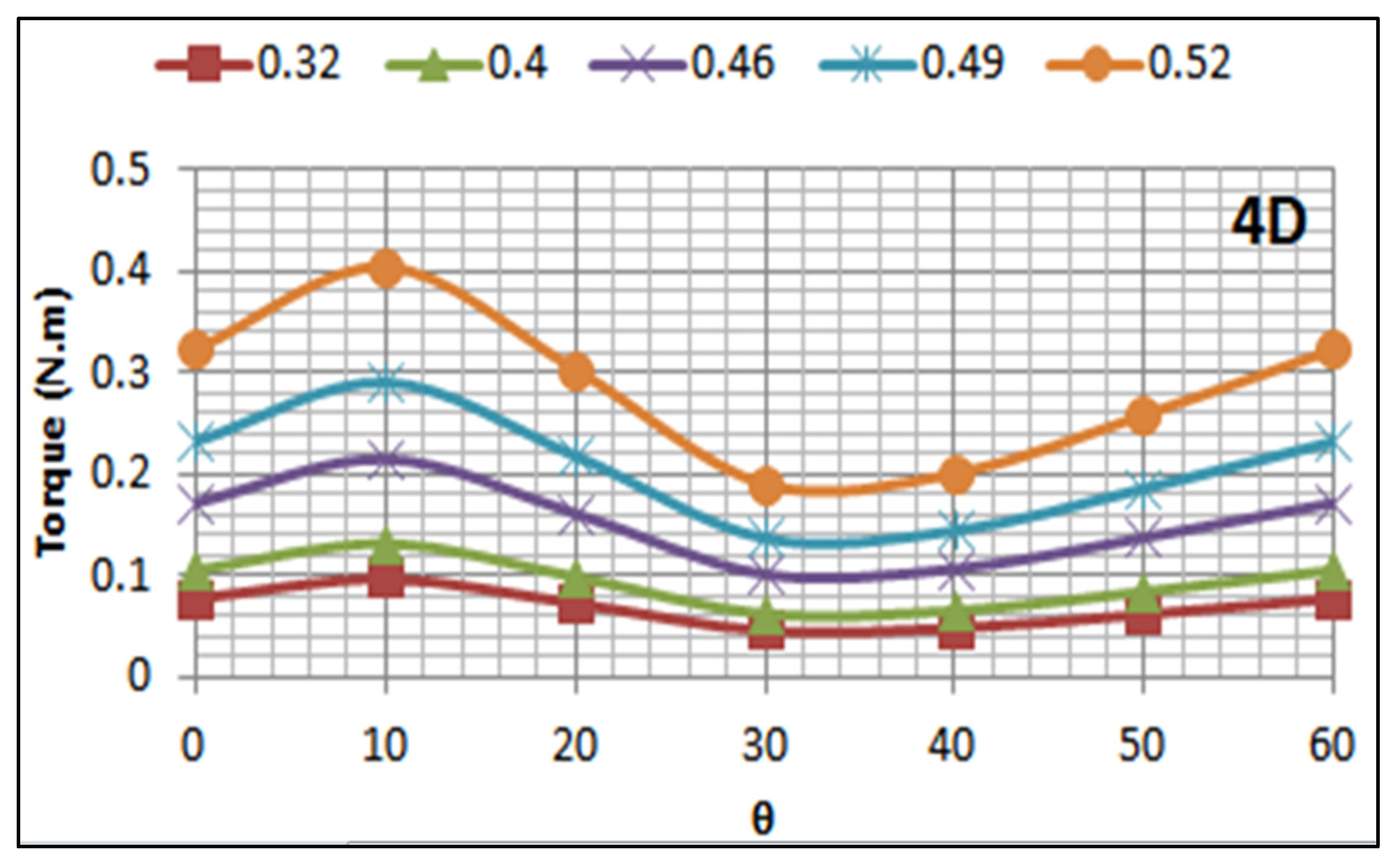
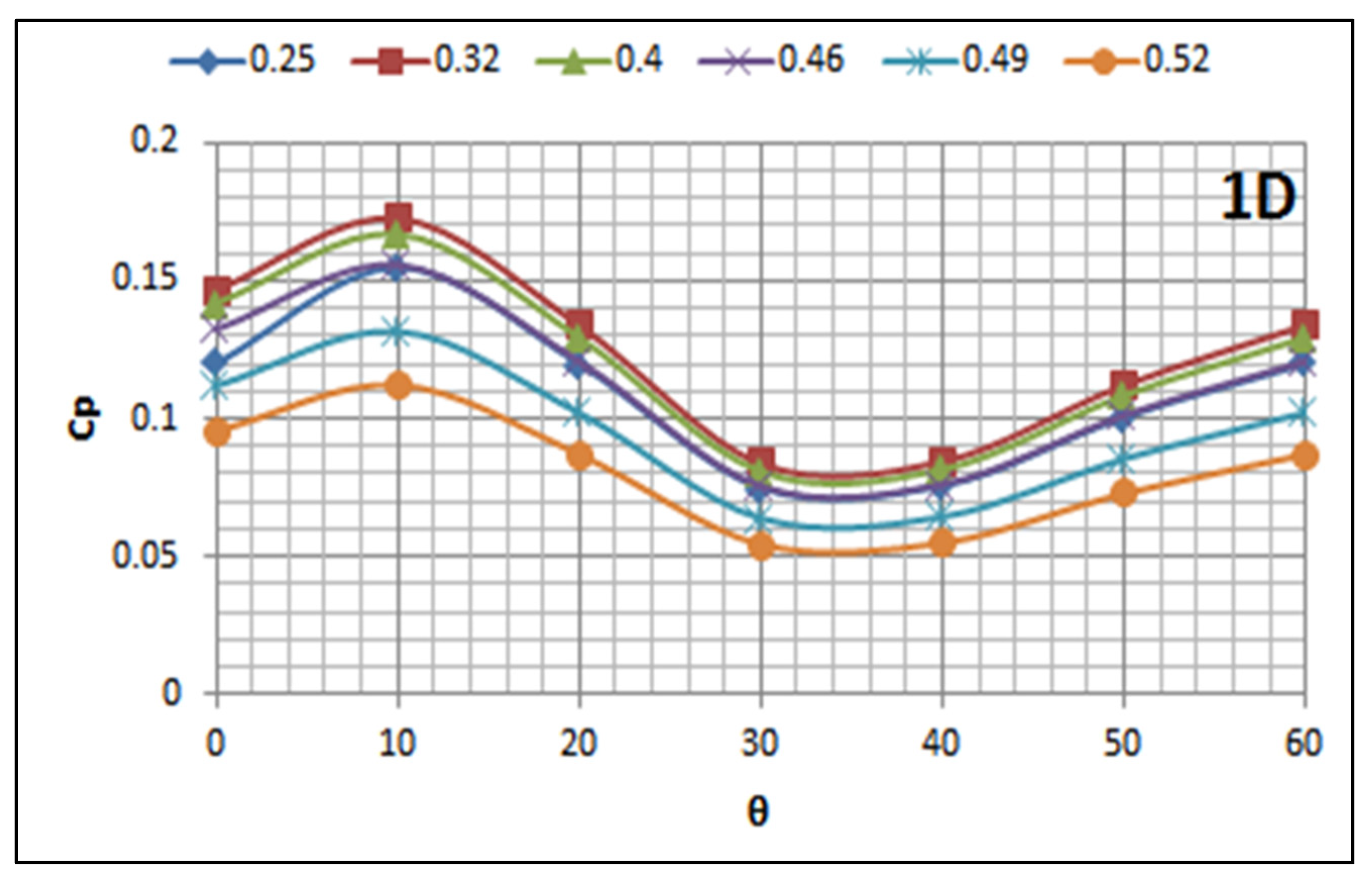
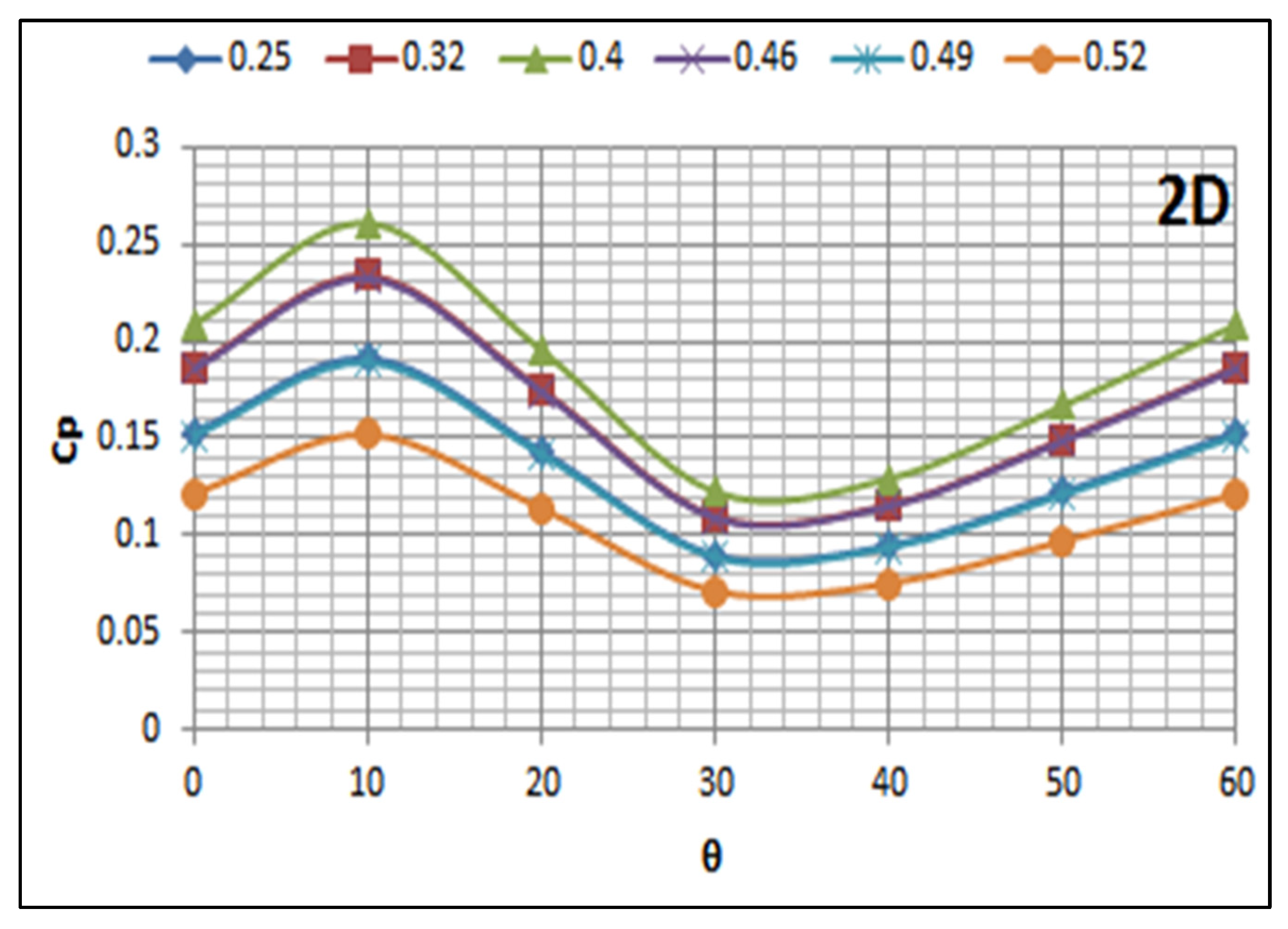
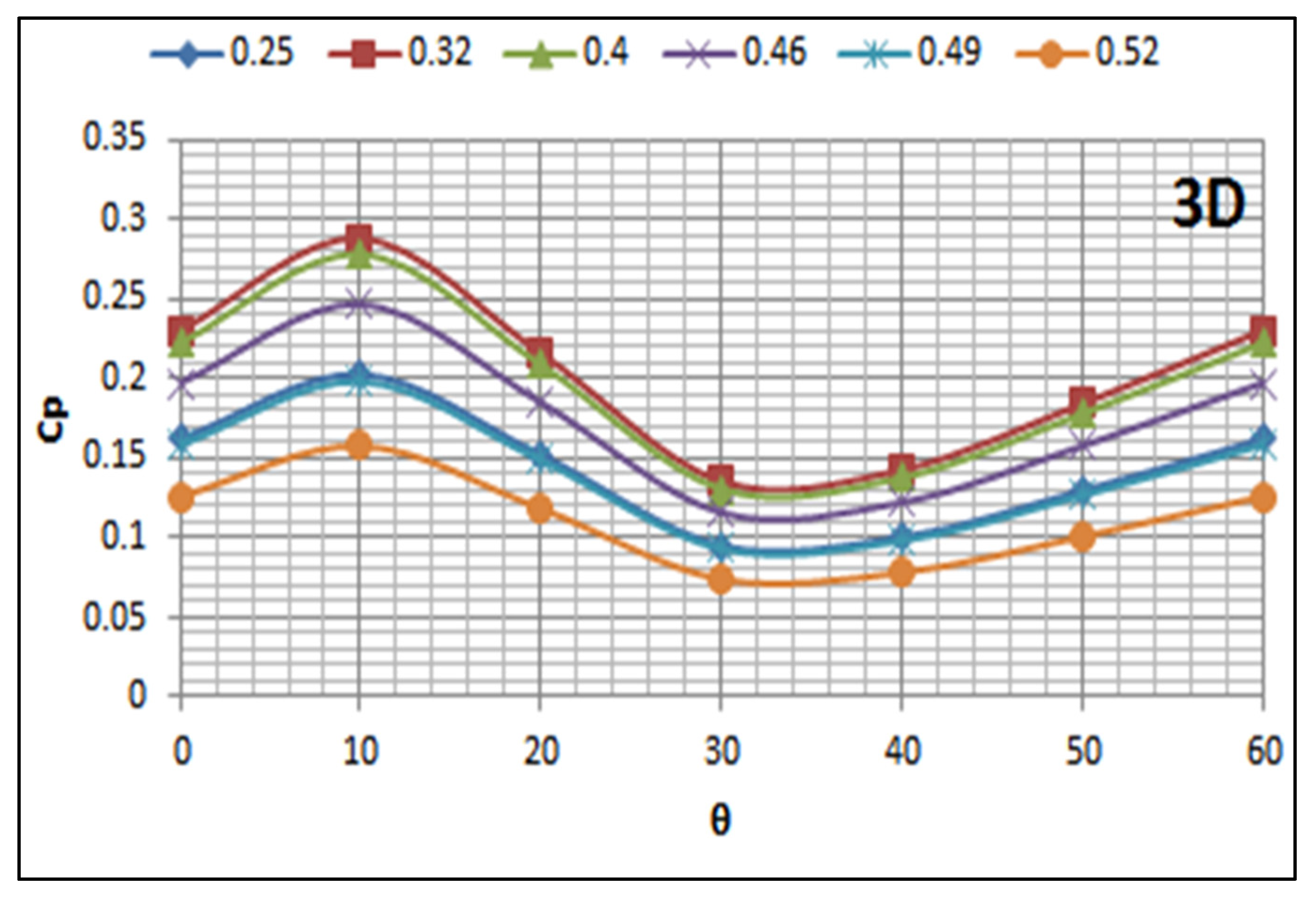
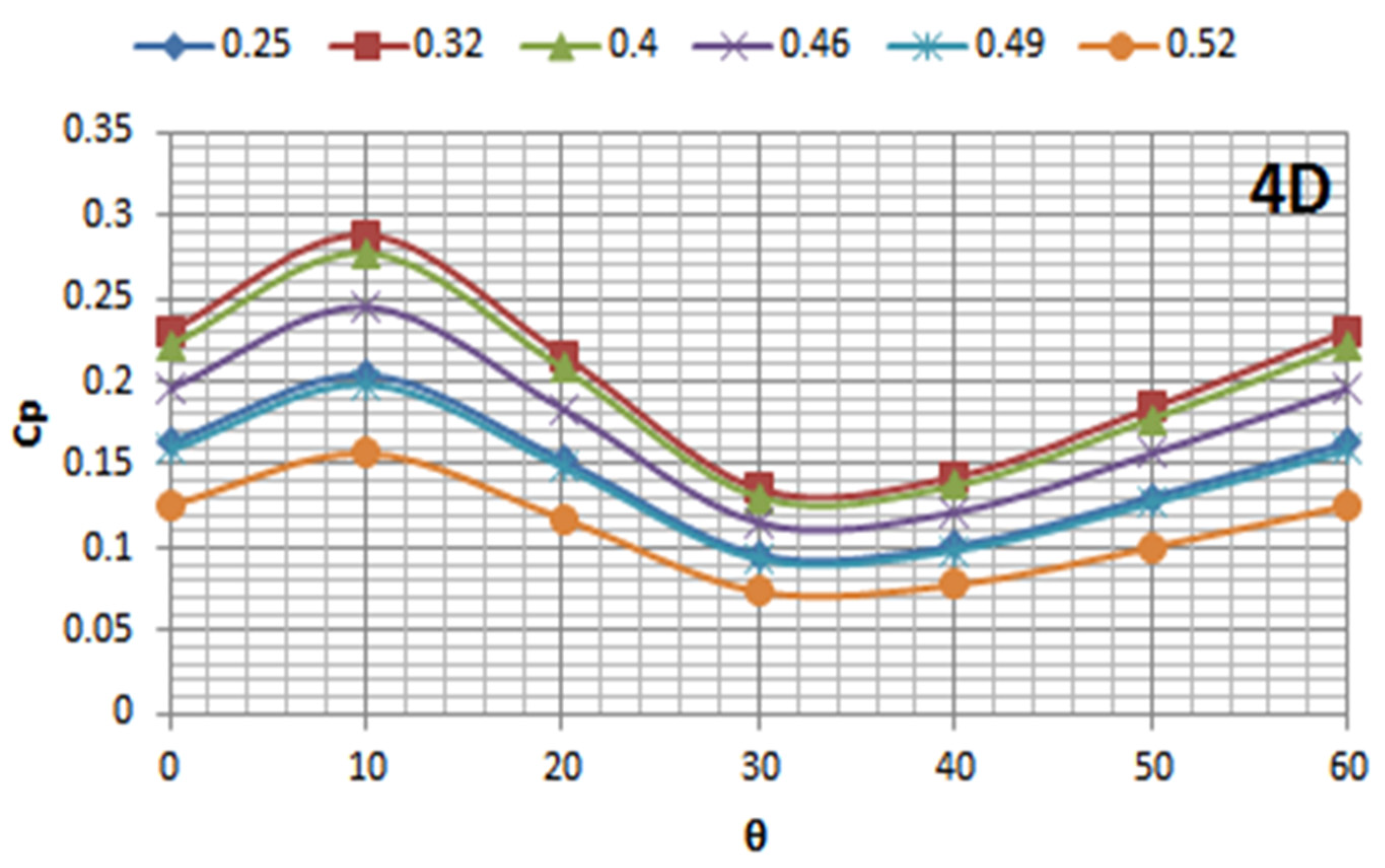
5.2. Effect of Turbine Submerged Depth on Its Performance
6. Conclusions
Author Contributions
Funding
Data Availability Statement
Conflicts of Interest
References
- Harries, T.; Kwan, A.; Brammer, J.; Falconer, R. Physical testing of performance characteristics of a novel drag-driven vertical axis tidal stream turbine; with comparisons to a conventional Savonius. Int. J. Mar. Energy 2016, 14, 215–228. [Google Scholar] [CrossRef] [Green Version]
- Kariman, H.; Hoseinzadeh, S.; Heyns, S.; Sohani, A. Modeling and exergy analysis of domestic MED desalination with brine tank. Desalin. Water Treat. 2020, 197, 1–13. [Google Scholar] [CrossRef]
- Mansour, A.E.; Pedersen, P.T.; Paik, J.K. Wave energy extraction using decommissioned ships. Ships Offshore Struct. 2013, 8, 504–516. [Google Scholar] [CrossRef]
- Kariman, H.; Hoseinzadeh, S.; Heyns, P.S. Energetic and exergetic analysis of evaporation desalination system integrated with mechanical vapor recompression circulation. Case Stud. Therm. Eng. 2019, 16, 100548. [Google Scholar] [CrossRef]
- Derakhshan, S.; Kasaeian, N. Optimization, Numerical, and Experimental Study of a Propeller Pump as Turbine. J. Energy Resour. Technol.-Trans. Asme 2014, 136, 012005. [Google Scholar] [CrossRef]
- Kariman, H.; Hoseinzadeh, S.; Shirkhani, A.; Heyns, P.S.; Wannenburg, J. Energy and economic analysis of evaporative vacuum easy desalination system with brine tank. J. Therm. Anal. Calorim. 2020, 140, 1935–1944. [Google Scholar] [CrossRef]
- Khan, M.J.; Bhuyan, G.; Iqbal, M.T.; Quaicoe, J.E. Hydrokinetic energy conversion systems and assessment of horizontal and vertical axis turbines for river and tidal applications: A technology status review. Appl. Energy 2009, 86, 1823–1835. [Google Scholar] [CrossRef]
- Martin-Short, R.; Hill, J.; Kramer, S.C.; Avdis, A.; Allison, P.A.; Piggott, M.D. Tidal resource extraction in the Pentland Firth, UK: Potential impacts on flow regime and sediment transport in the Inner Sound of Stroma. Renew. Energy 2015, 76, 596–607. [Google Scholar] [CrossRef] [Green Version]
- Sanchez, M.; Carballo, R.; Ramos, V.; Iglesias, G. Tidal stream energy impact on the transient and residual flow in an estuary: A 3D analysis. Appl. Energy 2014, 116, 167–177. [Google Scholar] [CrossRef]
- Chen, L.; Lam, W.H. A review of survivability and remedial actions of tidal current turbines. Renew. Sustain. Energy Rev. 2015, 43, 891–900. [Google Scholar] [CrossRef] [Green Version]
- Ma, Y.; Zhang, L.; Ma, L.; Chen, Z. Developing status and development trend of vertical axis turbine-type tidal current energy power generation device. Keji Daobao Sci. Technol. Rev. 2012, 30, 71–75. [Google Scholar]
- Batten, W.M.J.; Bahaj, A.S.; Molland, A.F.; Chaplin, J.R. The prediction of the hydrodynamic performance of marine current turbines. Renew. Energy 2008, 33, 1085–1096. [Google Scholar] [CrossRef]
- Li, Y.; Calisal, S.M. Numerical analysis of the characteristics of vertical axis tidal current turbines. Renew. Energy 2010, 35, 435–442. [Google Scholar] [CrossRef]
- Copping, A.; Hanna, L.; Whiting, J.; Geerlofs, S.; Grear, M.; Blake, K.; Coffey, A.; Massaua, M.; Brown-Saracino, J.; Battey, H. Environmental Effects of Marine Energy Development around the World; Annex IV Final Report; IEA Ocean Energy Systems Initiative, Annex IV: Richland, WA, USA, 2013. [Google Scholar]
- Jacobson, P.T.; Amaral, S.V.; Castro-Santos, T.; Giza, D.; Haro, A.J.; Hecker, G.; McMahon, B.; Perkins, N.; Pioppi, N. Environmental Effects of Hydrokinetic Turbines on Fish: Desktop and Laboratory Flume Studies; Electric Power Research Institute: Palo Alto, CA, USA, 2012. [Google Scholar]
- Yang, B.; Lawn, C. Fluid dynamic performance of a vertical axis turbine for tidal currents. Renew. Energy 2011, 36, 3355–3366. [Google Scholar] [CrossRef]
- Chen, B.; Cheng, S.B.; Su, T.C.; Zhang, H. Numerical investigation of channel effects on a vertical-axis tidal turbine rotating at variable speed. Ocean Eng. 2018, 163, 358–368. [Google Scholar] [CrossRef]
- Jing, F.M.; Sheng, Q.H.; Zhang, L. Experimental research on tidal current vertical axis turbine with variable-pitch blades. Ocean Eng. 2014, 88, 228–241. [Google Scholar] [CrossRef]
- Sun, J.J.; Huang, D.G. Numerical investigation on aerodynamic performance improvement of vertical-axis tidal turbine with super-hydrophobic surface. Ocean Eng. 2020, 217, 107995. [Google Scholar] [CrossRef]
- Derakhshan, S.; Ashoori, M.; Salemi, A. Experimental and numerical study of a vertical axis tidal turbine performance. Ocean Eng. 2017, 137, 59–67. [Google Scholar] [CrossRef] [Green Version]
- Maduka, M.; Li, C.W. Experimental evaluation of power performance and wake characteristics of twin flanged duct turbines in tandem under bi-directional tidal flows. Renew. Energy 2022, 199, 1543–1567. [Google Scholar] [CrossRef]
- Arcos, F.Z.D.; Vogel, C.R.; Willden, R.H.J. A parametric study on the hydrodynamics of tidal turbine blade deformation. J. Fluids Struct. 2022, 113, 103626. [Google Scholar] [CrossRef]
- Moreau, M.; Germain, G.; Maurice, G.; Richard, A. Sea states influence on the behaviour of a bottom mounted full-scale twin vertical axis tidal turbine. Ocean Eng. 2022, 265, 112582. [Google Scholar] [CrossRef]
- Sun, K.; Yi, Y.; Zhang, J.S.; Zhang, J.H.; Zaidi, S.S.H.; Sun, S.H. Influence of blade numbers on start-up performance of vertical axis tidal current turbines. Ocean Eng. 2022, 243, 110314. [Google Scholar] [CrossRef]
- Ma, Y.; Hu, C.; Li, L. Hydrodynamics and wake flow analysis of a Π-type vertical axis twin-rotor tidal current turbine in surge motion. Ocean Eng. 2021, 224, 108625. [Google Scholar] [CrossRef]
- Satrio, D.; Utama, I.K.A.P. Experimental investigation into the improvement of self-starting capability of vertical-axis tidal current turbine. Energy Rep. 2021, 7, 4587–4594. [Google Scholar] [CrossRef]
- Chen, Y.L.; Sun, J.; Lin, B.L.; Lin, J.; Guo, J.X. Spatial evolution and kinetic energy restoration in the wake zone behind a tidal turbine: An experimental study. Ocean Eng. 2021, 228, 108920. [Google Scholar] [CrossRef]
- Xie, J.M.; Chen, J.Y. Vertical-axis ocean current turbine design research based on separate design concept. Ocean Eng. 2019, 188, 106258. [Google Scholar] [CrossRef]
- Han, J.; Jung, J.; Hwang, J.H. Optimal configuration of a tidal current turbine farm in a shallow channel. Ocean Eng. 2021, 220, 108395. [Google Scholar] [CrossRef]
- Manolesos, M.; Chng, L.; Kaufmann, N.; Ouro, P.; Ntouras, D.; Papadakis, G. Using vortex generators for flow separation control on tidal turbine profiles and blades. Renew. Energy 2023, 205, 1025–1039. [Google Scholar] [CrossRef]
- Wang, P.Z.; Zhao, B.W.; Cheng, H.T.; Huang, B.; He, W.S.; Zhang, Q.; Zhu, F.W. Study on the performance of a 300W counter-rotating type horizontal axis tidal turbine. Ocean Eng. 2022, 255, 111446. [Google Scholar] [CrossRef]
- Samadi, M.; Hassanabad, M.G.; Mozafari, S.B. Performance enhancement of low speed current savonius tidal turbines through adding semi-cylindrical deflectors. Ocean Eng. 2022, 259, 111873. [Google Scholar] [CrossRef]
- Khanjanpour, M.H.; Javadi, A.A. Optimization of a Horizontal Axis Tidal (HAT) turbine for powering a Reverse Osmosis (RO) desalination system using Computational Fluid Dynamics (CFD) and Taguchi method. Energy Convers. Manag. 2021, 231, 113833. [Google Scholar] [CrossRef]
- Yang, B.; Lawn, C. Three-dimensional effects on the performance of a vertical axis tidal turbine. Ocean Eng. 2013, 58, 1–10. [Google Scholar] [CrossRef]
- Wang, X.L.; Qiao, D.S.; Jin, L.X.; Yan, J.; Wang, B.; Li, B.B.; Ou, J.P. Numerical investigation of wave run-up and load on heaving cylinder subjected to regular waves. Ocean Eng. 2023, 268, 113415. [Google Scholar] [CrossRef]
- Liang, H.Z.; Qiao, D.S.; Wang, X.Z.; Zhi, G.N.; Yan, J.; Ning, D.Z.; Ou, J.P. Energy capture optimization of heave oscillating buoy wave energy converter based on model predictive control. Ocean Eng. 2023, 268, 113402. [Google Scholar] [CrossRef]
- Wang, Z.M.; Qiao, D.S.; Yan, J.; Tang, G.Q.; Li, B.B.; Ning, D.Z. A new approach to predict dynamic mooring tension using LSTM neural network based on responses of floating structure. Ocean Eng. 2022, 249, 110905. [Google Scholar] [CrossRef]
- Nazarieh, M.; Kariman, H.; Hoseinzadeh, S. Numerical simulation of fluid dynamic performance of turbulent flow over Hunter turbine with variable angle of blades. Int. J. Numer. Methods Heat Fluid Flow 2023, 33, 153–173. [Google Scholar] [CrossRef]


| Velocity (m/s) | Power (w)—Exp. | Power (w)—Nu. |
|---|---|---|
| 0.4 | 0.017 | 0.09 |
| 0.7 | 0.11 | 0.17 |
| 0.8 | 0.19 | 0.29 |
| 1 | 0.44 | 0.53 |
| 1.2 | 0.58 | 0.78 |
| 1.4 | 0.89 | 1.06 |
Disclaimer/Publisher’s Note: The statements, opinions and data contained in all publications are solely those of the individual author(s) and contributor(s) and not of MDPI and/or the editor(s). MDPI and/or the editor(s) disclaim responsibility for any injury to people or property resulting from any ideas, methods, instructions or products referred to in the content. |
© 2023 by the authors. Licensee MDPI, Basel, Switzerland. This article is an open access article distributed under the terms and conditions of the Creative Commons Attribution (CC BY) license (https://creativecommons.org/licenses/by/4.0/).
Share and Cite
Ghamati, E.; Kariman, H.; Hoseinzadeh, S. Experimental and Computational Fluid Dynamic Study of Water Flow and Submerged Depth Effects on a Tidal Turbine Performance. Water 2023, 15, 2312. https://doi.org/10.3390/w15132312
Ghamati E, Kariman H, Hoseinzadeh S. Experimental and Computational Fluid Dynamic Study of Water Flow and Submerged Depth Effects on a Tidal Turbine Performance. Water. 2023; 15(13):2312. https://doi.org/10.3390/w15132312
Chicago/Turabian StyleGhamati, Erfan, Hamed Kariman, and Siamak Hoseinzadeh. 2023. "Experimental and Computational Fluid Dynamic Study of Water Flow and Submerged Depth Effects on a Tidal Turbine Performance" Water 15, no. 13: 2312. https://doi.org/10.3390/w15132312