Article

Effect of Different Water Treatments in Soil-Plant-Atmosphere Continuum Based on Intelligent Weighing Systems

1
College of Agricultural Engineering, Shanxi Agriculture University, Jinzhong 030801, China
2
National Engineering Research Center for Intelligent Equipment in Agriculture, Beijing Academy of Agriculture and Forestry Sciences, Beijing 100097, China
3
Key Laboratory for Quality Testing of Hardware and Software Products on Agricultural Information, Ministry of Agriculture, Beijing 100125, China
4
Beijing Agricultural Technology Promotion Station, Beijing 100029, China
5
Tianjin Agricultural Machine Technology Test Service Center, Tianjin 301616, China
*
Authors to whom correspondence should be addressed.
Water 2022, 14(4), 673; https://doi.org/10.3390/w14040673
Submission received: 20 January 2022 / Revised: 10 February 2022 / Accepted: 16 February 2022 / Published: 21 February 2022
(This article belongs to the Special Issue Numerical Modeling of Water Flow, Nutrients and Sediment Transport)

Abstract

:
In order to meet the needs of dynamic continuous monitoring of soil-plant-atmosphere continuum (SPAC), a new soil, plant, atmosphere analysis system has been established based on an intelligent weighing system (IWS). Four types of irrigation treatments (90%, 80%, 70%, and 60% of field capacity (FC)) were conducted on lettuce (Lactuca sativa var. ramosa Hort.) for two-season planting experiments. Regarding the soil, the relative system weight of IWS showed a significant linear correlation with the soil volumetric moisture content (SWC) (R2 = 0.64–0.94). When the SWC increased by 1.00%, the soil weight increased by 56–62 g. Regarding plants, the IWS also clearly reflected the changes in plant weight gain, transpiration rate, and stomatal conductance at different growth stages. After verification, the relative errors of the transpiration rate and stomatal conductance measured by the IWS were −9.60–22.30% and −7.20–22.20%, respectively. Regarding the atmospheric environment, the variation trend of the crop evapotranspiration (ETc) based on the IWS and the reference crop evapotranspiration (ET0) calculated with meteorological parameters were consistent. However, the numerical difference was in the uncertainty of the crop coefficient (Kc). The ETc of lettuce under the 80% FC treatment was the highest. Accordingly, a daily online measurement method for Kc was established. The Kc values of lettuce at different growth stages were 0.88, 1.22, and 2.43, respectively. The growth, yield, and water use efficiency (WUE) of crops under 80% FC treatment compared with other treatments significantly increased by 11.07–21.05%, 0.91–9.89%, and 2.16–15.80%, respectively. Therefore, the 80% FC was adopted as the irrigation low limit of potted lettuce. The experimental results provide a theoretical basis for further guiding crop irrigation.

1. Introduction

In the SPAC water vapor dynamic circulation system, plants are the main link connecting soil and atmosphere [1,2,3,4,5]. Water reaches plant roots through soil, leaves through plant stems, then diffuses from leaf stomata to the static air layer, and finally participates in the atmospheric turbulent transformation to form a unified, dynamic, and mutual feedback continuous system [6,7]. Accordingly, the continuous monitoring of SPAC is of great significance for comprehensively exploring the law of crop water consumption.
Domestic and foreign scholars have conducted extensive research on SPAC. In the field of soil monitoring, Ekanayaka et al. [8] have developed low-cost capacitive soil moisture sensors for data collection, with the aim of automatically monitoring soil moisture. Shen et al. [9] used soil moisture sensors to measure the soil moisture content at different depths to determine the appropriate placement of soil moisture sensor. Stephan et al. [10] utilized soil moisture sensors to measure the soil moisture content at different locations and found that after rainfall, the soil moisture in the corridor was the lowest in the weathered surface crust. However, in practical application, the aforementioned methods can only obtain single-point parameters and cannot completely describe the state of the overall soil moisture loss in the root-zone during crop growth. In crop monitoring, a portable photosynthetic instrument is utilized to determine the transpiration rate, stomatal conductance and other indicators of cotton [
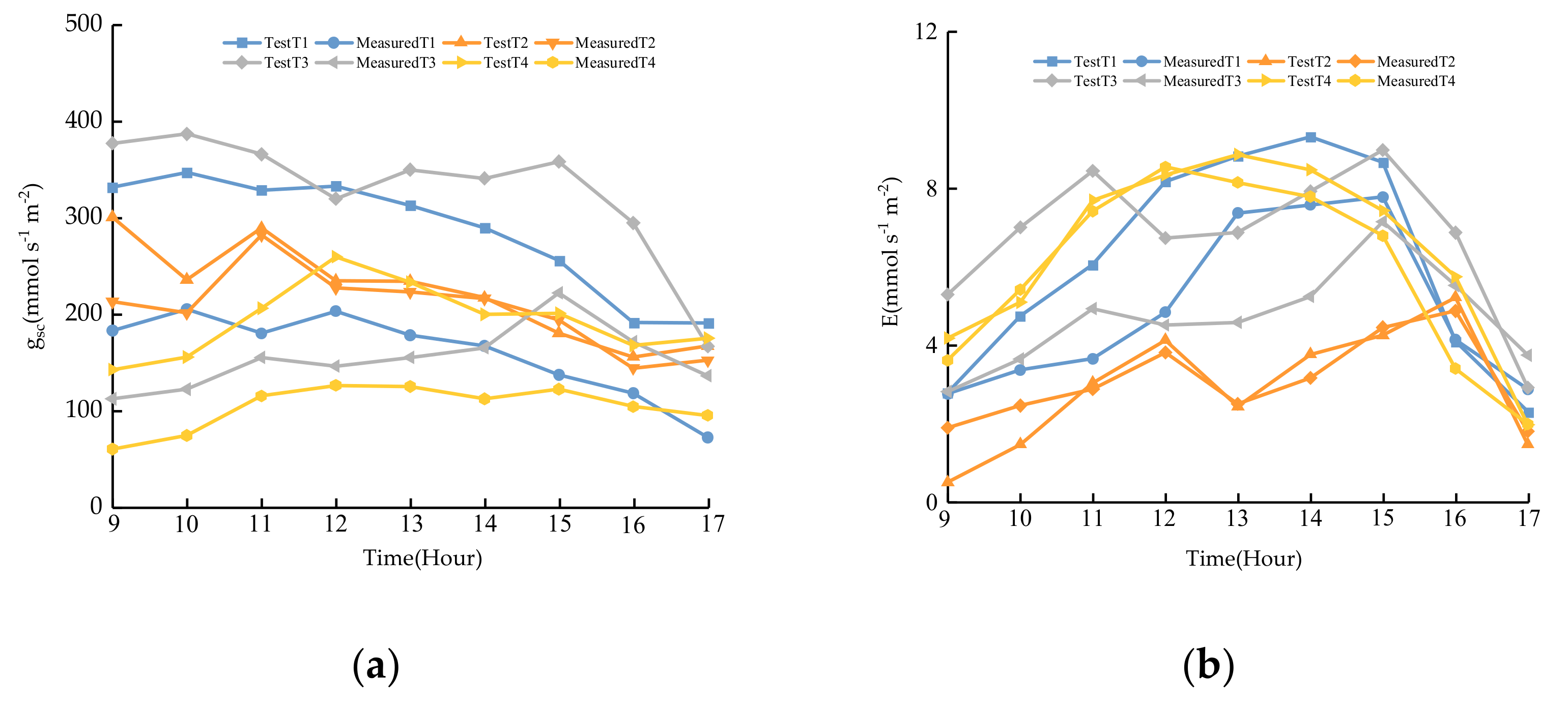
11], hybrid winter wheat [12] and young apricot trees [13]. Current monitoring methods are mainly based on leaf-scale parameter information, and continuous online monitoring cannot be realized, thereby reducing the integrity of crop response research. Regarding atmospheric monitoring, Liu et al. [14] and Wang et al. [15] utilized a large-scale automatic weighing lysimeter to measure the actual crop evapotranspiration. Tyagi et al. [16] used a weighing lysimeter to measure the hourly evapotranspiration of rice and sunflowers. However, the equipment has high cost, complicated installation, and difficult soil borrowing process, thereby limiting its wide-scale application.
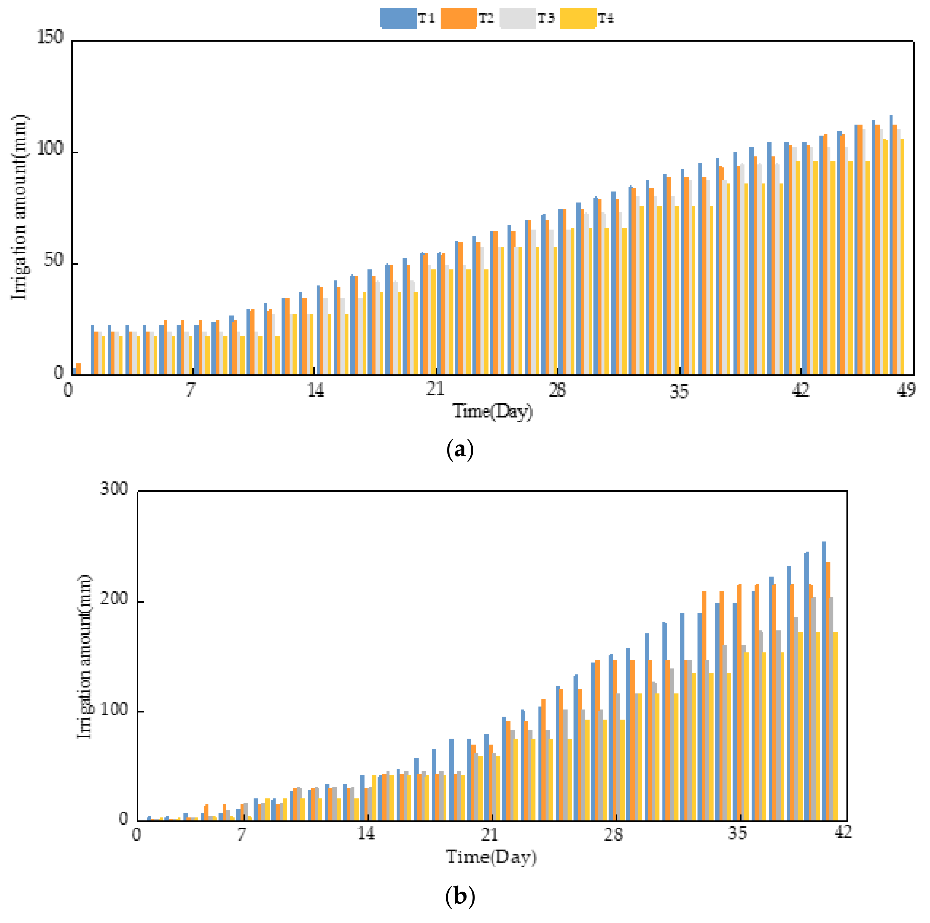
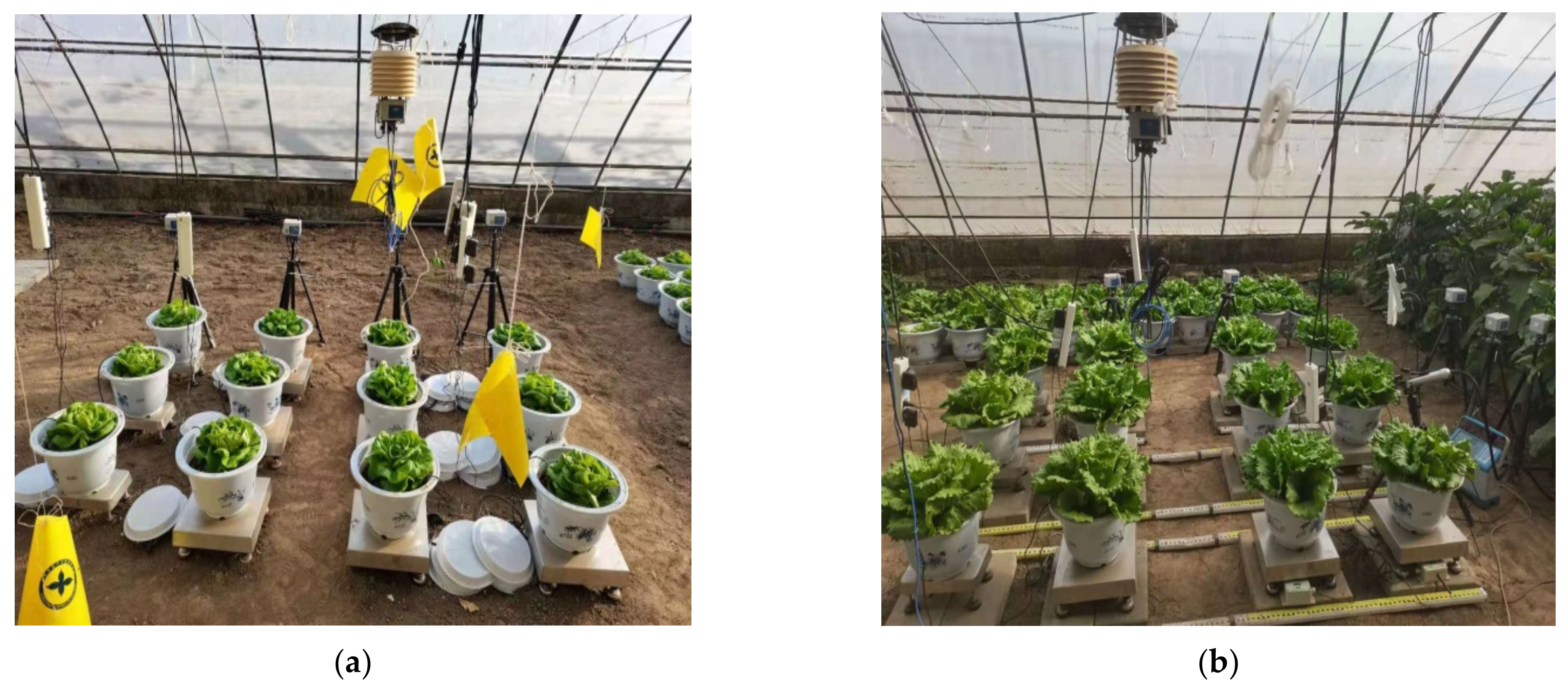
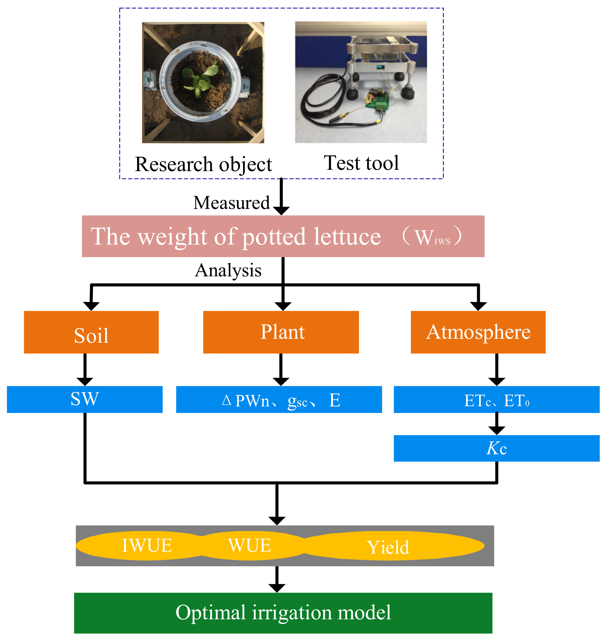
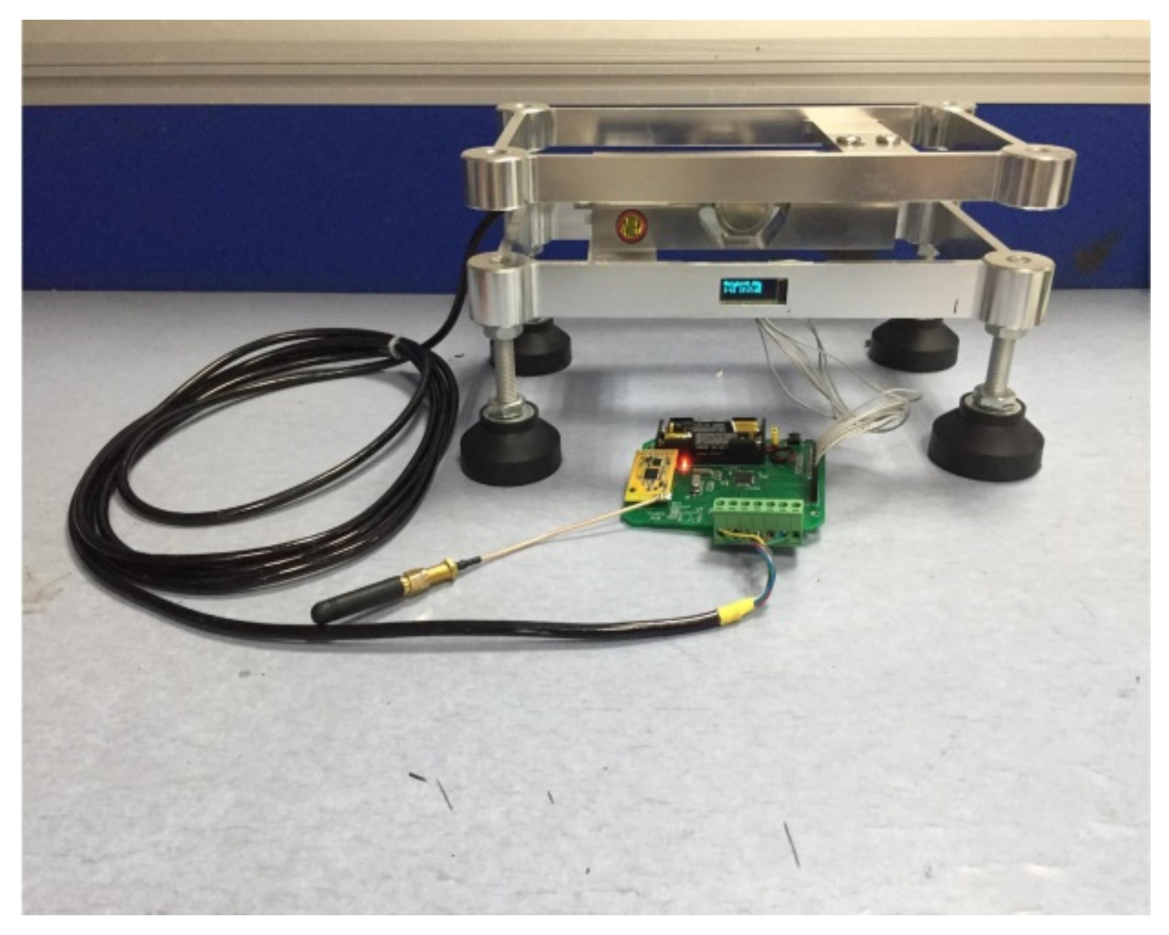
Based on this, we propose a low-cost potted plant evapotranspiration measurement system based on Lora wireless technology for horticultural facilities [17]. This system achieves the continuous weighing of potted plants in the whole growth cycle and real-time monitoring of the evapotranspiration of potted plants. As a kind of crop with large water demand and high sensitivity to water, vegetables are suitable for irrigation test based on our IWS. Lettuce (Lactuca sativa var. ramosa Hort.) as a representative of leafy vegetables, is rich in nutrition and has certain health and medicinal value. In recent years, the cultivation scale of lettuce has increased rapidly. The vegetable planting area in China is approximately 1.35 million hm2 [18]. Based on the IWS, this study monitors and analyzes the SPAC of lettuce under different water treatments, so as to explore the water consumption characteristics of potted crops under different water treatments. This study provides theoretical guidance for improving precise crop irrigation and provides a new direction for the development of irrigated agriculture.

2. Materials and Methods

2.1. Test Materials

This study conducted two cropping experiments in a sunlight greenhouse (116°46′ E, 40°18′ N) of the National Precision Agriculture Demonstration Base in Changping District, Beijing, at an altitude of 50 m. Pot planting of lettuce (Lactuca sativa var. ramosa Hort.) was used in the experiments. Soil was obtained from 0–20 cm soil layer of the base farmland. After being naturally air dried it was crushed and passed through a 2-mm sieved soil. The soil type was sandy clay loam and the cultivated land quality grade is medium. The field water capacity was measured by the drying method, and the soil bulk density was measured by the Wilkes method [19]. The inner diameter of the pot used in the experiments was 29 cm, and the height was 23 cm. The pot was filled with 8 kg of air-dried soil. Before planting, 1.57 g of urea (containing 46% N), 1.53 g of diamine phosphate (containing 12% N, 42% P2O5), and 1.54 g of potassium sulphate (containing 52% K2O) were applied as the base fertilizer and combined with the soil by mixing well.
There are two types of lettuce: leaf-expansion lettuce and heading lettuce. In the first season experiment, six-leaf and one-heart-stage lettuce was selected for colonization on 4 September 2020, with one plant per pot. The lettuce variety was leaf-expansion (Boston butter lettuce), the FC was 29.75% (volume percentage), and the soil bulk density was 1.21 g·cm−3. In the second season experiment, six-leaf and one-heart-stage lettuce was selected for colonization on 1 April 2021, with one plant per pot. The lettuce variety was heading lettuce (Italian Sagittarius 101 head lettuce), the FC was 31% (volume percentage), and the soil bulk density was 1.36 g·cm−3.

2.2. Experimental Design

Four different water treatments were set up in the experiments as summarized in Table 1. The SWC was monitored by a soil moisture sensor. In this study, four different irrigation low limit treatments were carried out, with 100% as irrigation maximum and 90% (T1), 80% (T2), 70% (T3), and 60% (T4) as irrigation low limit respectively. When the SWC decreased to the irrigation low limit, irrigation was performed to ensure that the SWC reaches the irrigation maximum. The irrigation quota was calculated in accordance with the national micro-irrigation technical standard [20]. The irrigation time and the amount of irrigation during the first and second seasons are illustrated in Figure 1. In the experiment, 52 pots were set for each planting season, of which 12 pots were placed on the scale, and 3 replicates were set for each treatment. The test arrangement is illustrated in Figure 2.

2.3. Measurement Items and Methods

2.3.1. SWC

The first season experiment used the EC—5 soil moisture sensor produced by Decagon in the United States. The measurement accuracy is ±1–2% SWC. The second season experiment used the TEROS12 soil moisture sensor produced by the US METER company. The resolution is 0.001 m3/m3, and the accuracy is ±1–2% SWC. The sensor was inserted near the root of the lettuce, with the depth of the probe into the soil of 5.5 cm. The change of SWC was monitored in real time and was collected automatically once every hour.

2.3.2. Environmental Parameters

The experiments used the greenhouse cloud environment EP400 data collector developed by the National Engineering Research Center for Intelligent Equipment in Agriculture for environmental monitoring. The data collector can detect air temperature (range: –40 to 80 °C, accuracy: ±0.5 °C), relative air humidity (range: 0–100%, accuracy: ±3%), and light intensity (range: 0–100 klx, accuracy: ±10 klx). Meteorological data were automatically collected hourly. The maximum and minimum air temperatures at the test site were recorded daily.

2.3.3. Plant Parameters

The CIRAS-3 photosynthetic apparatus produced by PP Systems was used to test the data from 9:00 to 17:00 on a sunny day. The second fully expanded leaf from top to bottom was selected to measure the transpiration rate and stomatal conductance of the leaves.

2.3.4. ET0

The FAO-56 Penman–Monteith equation, based on microclimatology and energy balance, is the most practical and reliable method for calculating crop evapotranspiration. Satisfactory results have been obtained in experimental research of crop evapotranspiration infield and greenhouse. This greenhouse experiment uses the revised Penman–Monteith formula [21]. The calculation formula is as follows:
E T 0 = 0.408 Δ R n G + γ 1713 e s e a T + 273 Δ + 1.64 γ
where ET0 represents the reference crop evapotranspiration (mm/d); Rn is net radiation of the crop canopy (MJ/(m2 d)); G is the soil heat flux density (MJ/(m2 d)); T is the daily average temperature at a height of 1.5–2.5 m above the ground (°C); es is the average saturated vapor pressure at 1.5–2.5 m above the ground (kPa); ea is the average actual vapor pressure at a height of 1.5–2.5 m above the ground (kPa); ∆ is the slope of the saturated vapor pressure curve (kPa/°C), and γ is the wet and dry constants of values, 0.067 kPa/°C.

2.3.5. Kc

Kc refers to the ratio of the actual water consumption during the growth stage to the reference crop evapotranspiration. The calculation formula is as follows:
K c = E T c E T 0
where Kc is the crop coefficient, ET0 is the reference crop evapotranspiration during the growth period of the crop (mm/d), and ETc is the water consumption at the crop stage during the growth period of the crop (mm/d).

2.3.6. Saturated Water Vapor Pressure Deficit (VPD)

VPD is the difference between the saturated water vapor pressure of the ambient air and the actual water vapor pressure, which affects the closure of the crop stomata. It is commonly used to evaluate atmospheric water demand. Its calculation formula is as follows:
V P D = 0.611 × e 12.27 T a 237.3 + T a × 1 R H 100
where VPD is the saturated vapor pressure of the air (kPa), Ta is the atmospheric temperature (°C), and RH is the relative humidity of the air (%).

2.4. Pearson Correlation

Pearson correlation coefficient is often used to detect whether the independent and dependent variables are correlated. The value ranges from −1 to 1, and the formula is as follows:
P xy = ( x x ¯ ) y y ¯ x x ¯ 2 y y ¯ 2
where, x x ¯ y y ¯ is the covariance between variable x and variable y, x x ¯ 2 y y ¯ 2 is the standard deviation between variable x and variable y, P x y is the correlation coefficient. The greater the absolute value of the correlation coefficient, the stronger the correlation. The closer the correlation coefficient is to 1 or −1, the stronger the correlation is; the closer the correlation coefficient is to 0, the weaker the correlation is Ref. [22].

2.5. Parameter Calculation Module of IWS

The IWS can continuously monitor plants online in real time. According to the changes of weight (WIWS), the IWS can analyze the daily evapotranspiration (ET), weight gain change (ΔPWn), instantaneous whole plant transpiration rate (E), and stomatal conductance (gsc) of plants [23,24].
E T C = W m W e
where ETc is the difference between the readings of the IWS at 00:00 of the present day and that at 00:00 of the next day (g), Wm is the average weight of the two sampling moments before and after 00:00 of the day (g), We is the average weight of the two sampling moments before and after 00:00 the next day (g).
Δ P W n = W n W n 1
where ΔPWn can be calculated by the difference of the weight between the nth irrigation and the n − 1th irrigation (g), Wn is the average weight of the two sampling times before and after the nth irrigation (g), Wn−1 is the average weight of the two sampling times before and after the n − 1th irrigation (g).
E = d W d t k W k W k 1 t k t k 1
where E is obtained by multiplying the first derivative of the measured time series by −1 (g h−1), Wk is the IWS reading when time is tk (g), Wk−1 is the IWS reading when the time is tk−1(g). The weight gain of the plant in the short time interval, which is used to calculate the transpiration rate, is assumed to be negligible. Under the condition of soil water deficit, the WUE of the plant changes very little. Hence, it can be neglected.
g s c = E P a t m L A V P D
where gsc is calculated as the ratio of the transpiration rate of the entire plant, the atmospheric pressure to the leaf surface area and the saturated vapor pressure deficit (mmol m−2 s−1), P a t m is the atmospheric pressure (101.3 kPa), E is the transpiration rate (g h−1), LA is the leaf surface area (m2), VPD is the saturated water vapor pressure deficit (KPa).

2.6. Data Analysis

Data analysis was performed by SPSS software, chart drawings were created by Origin software, data processing was conducted by Excel software, and significance analysis was conducted by performing one-way analysis of variance.

2.7. Technical Roadmap

The experimental technical roadmap is illustrated in Figure 3, which includes the following steps: 1. With lettuce as the research object and IWS as the tool, the weight of potted lettuce (WIWS) is measured according to the IWS; 2. According to WIWS, the characteristic parameters of soil (soil moisture weight [SW]), plant ([ΔPWn], [gsc], [E]), and atmosphere (ETc) are analyzed. Kc is calculated from ETc and ET0; 3. The optimal irrigation model is obtained by comparing irrigation water use efficiency (IWUE), WUE, and yield.

3. Results

3.1. Hardware Design Module of IWS

Figure 4 illustrates the hardware structure of the IWS developed by Beijing Research Center for Intelligent Equipment in Agriculture. It includes six parts: the main controller, power supply, data collection, data display, data storage, and communication module. The main controller uses STM32′s low-power series L431CCT6, which can coordinate the normal operation of various components. The power supply uses TI’s TPS61221 boost chip to convert the 3 V voltage provided by the dry battery to an operating voltage of 3.3 V required by the system. For data collection, the HX712 electronic scale-dedicated high-precision A/D conversion chip from Haixin Technology Co., Shenzhen, China is used to collect the weight information. The data display adopts a 0.91 inch OLED with an SSD1306 controller, which can display the real-time weight and time of the scale. Data storage uses NOR flash type W25Q64, which is used to store system parameters and backup the real-time weight and time of the collection scale. The communication module adopts low-power wide-area network technology for data transmission between nodes and industrial tablet computers [17].

3.2. Analysis of the Changes of Soil Moisture Content under Different Water Treatments Based on IWS

Figure 5a illustrates the change trend of the relative weight of the IWS during the entire growth period under different water treatments (RW is the ratio of the weight at different weighing times to the weight at the beginning). The IWS can accurately reflect the changes in the weight of potted plants at different times during different growth periods. The direction of the arrow indicates the time of irrigation, and the increase in the dotted line indicates an increase in plant weight. With the change of the irrigation amount, RW fluctuates. The fluctuation range of soil moisture under T1 treatment is significantly smaller than that of the other treatments. This is because the single irrigation amount of T1 treatment is small. As the growth period progresses, the frequency of irrigation gradually increases. In the early stage of seedlings, lettuce is not processed because of soil moisture irrigation. During the rosette stage, the leaf area of lettuce increases, the water consumption increases as well, and the peak moments are different under different water treatments. At the end of heading, the lettuce is close to maturity, the water demand decreases, and the frequency of changes in RW decreases as well. During the entire growth period, in the first season experiment, the RW intervals of T1, T2, T3, and T4 are 0.95–1.08, 0.94–1.06, 0.93–1.06, and 0.92–1.05, respectively. The RW ranges of T1, T2, T3, and T4 in the second season are 0.90–1.14, 0.89–1.14, 0.89–1.11, and 0.89–1.10, respectively.
Figure 5b illustrates the change trend of SWC during the entire growth period under different water treatments. The SWC of lettuce fluctuates under different water treatments. In the first season, the upper limit of SWC for T1, T2, T3, and T4 is 29.75%, and the irrigation low limit is 26.77%, 23.80%, 20.82%, and 17.85%, respectively. In the second season, the upper limit of SWC for T1, T2, T3, and T4 is 31.00%, and the irrigation low limit is 27.90%, 24.80%, 21.70%, and 18.60%, respectively. When the SWC of T1, T2, T3, and T4 drops to the corresponding lower limit, the irrigation will be performed until the SWC reaches the irrigation maximum. The figure illustrates that the first season experiment belongs to the autumn stubble. As the temperature decreases, the water consumption of lettuce decreases, and the frequency of SWC fluctuations gradually decreases as well. The second season test is spring stubble. As the temperature increases, the water consumption of lettuce increases, and the frequency of SWC fluctuations gradually increases as well. The average soil moisture content is the lowest under T4 treatment and is in a long-term low-moisture state.
The IWS is more consistent with the change trend of the SWC. The maximum and minimum values of SWC correspond to the moments when the maximum and minimum values of WIWS appear, which indicates that the IWS can sensitively describe the influence of soil moisture changes.
Linear regression analysis is used to fit the WIWS and SW of four irrigation low limit treatments to further explore the accuracy of WIWS response to SW under different water treatments. As illustrated in Figure 6, the fitting effect of WIWS and its corresponding SW under the four gradients in the first and second seasons is quite good, reaching a significant level of 5%. The determination coefficients for the first and second seasons are 0.87, 0.87, 0.94, 0.85, and 0.64, 0.73, 0.70, 0.76, respectively (Table 2). Overall, because the weight of the lettuce in the second season is more than three times of that in the first season, the weight symmetry of the lettuce has a higher influence. For a similar water weight in the soil, the weight of the scale varies widely. Therefore, the coefficient of determination in the second season is lower than that in the first season.

3.3. Growth Analysis under Different Water Treatments Based on IWS

Figure 7 illustrates the change trend of lettuce weight gains under different water treatments. According to the IWS, ΔPWn and cumulative weight gain (ΣPWn) of lettuce are calculated, which can clearly reflect the growth of lettuce in different growth periods, and describe the weight change of lettuce throughout the growth cycle. The figure indicates that ΔPWn generally increases first and then gradually decreases. Under different water treatments, the weight gain rates of T1, T2, T3, and T4 in the first season are 7.37 g/d, 8.27 g/d, 7.80 g/d and 7.08 g/d, respectively. The weight gain rates of T1, T2, T3, and T4 in the second season are 29.75 g/d, 33.03 g/d, 22.99 g/d, and 20.26 g/d, respectively. In the first season, the ΔPWn of the lettuce under the T2 treatment is the highest in the seedling and rosette stages, and the ΔPWn of the lettuce under the T3 treatment is the highest in the late heading stage. During each growth period of lettuce in the second season, ΔPWn is the highest under T2 treatment. Overall, lettuce has the fastest weight gain rate under T2 treatment, and ΔPWn is the highest. At the end of the growth period, the ΣPWn of T1, T2, T3, and T4 in the first season is 361 g, 405 g, 382 g, and 347 g, respectively. The ΣPWn of T1, T2, T3, and T4 in the second season is 1239.67 g, 1417.34 g, 965.87 g, and 851.167 g respectively. At the 5% significance level, the differences between the different treatments are significant.
Null hypothesis means that there is no significant difference in the mean values of the controlled variables observed at different levels, that is, there is no significant difference in the mean values of experimental results under four different water treatments. Partial results of one-way ANOVA are shown in Table 3. The significance of lettuce weight gain in the first season is 0.00 and 0.02 in the second season. Both are less than 0.05. At the significance level of 0.05, the probability value p is lower than 0.05, so the null hypothesis is not valid. It is believed that if the overall mean values of the observed variables are different at different levels, then the different water treatments have significant effects on the weight gain of lettuce.

3.4. Physiological Analysis under Different Water Treatments Based on IWS

Figure 8 illustrates the E of the whole lettuce during the entire growth period under different water treatments. To eliminate the influence of lettuce size on E, we normalize it to the leaf surface area. The figure illustrates that during the entire growth period, E exhibits a significant fluctuating change. As the growth period progresses, lettuce E gradually decreases. Under different water treatments, the hourly average E during the entire growth period of T1, T2, T3, and T4 in the first season is 2.43 g·h−1, 2.57 g·h−1, 2.35 g·h−1 and 2.02 g·h−1. The average hourly E during the entire growth period of T1, T2, T3 and T4 in the second season is 2.23 g·h−1, 2.29 g·h−1, 2.22 g·h−1, and 2.12 g·h−1, respectively. The research results in the first and second seasons indicate that E is at its lowest value for a long time under T4 treatment. At the 5% significance level, the differences between the different water treatments are significant.
gsc is the main channel for gas exchange between plant leaves and the outside world, and the degree of stomatal dispersion has a direct effect on transpiration. Figure 9 illustrates the change trend of the gsc of lettuce under different water treatments. Generally, the gsc of lettuce decreases gradually, and gsc decreases significantly in the late seedling stage. Under different water treatments, the average hourly gsc of T1, T2, T3, and T4 in the first season are 364.53 mmol m−2 s−1, 396.48 mmol m−2 s−1, 326.48 mmol m−2 s−1, and 300.60 mmol m−2 s−1, respectively. The average hourly gsc of T1, T2, T3, and T4 in the second season are 180.32 mmol m−2 s1, 186.85 mmol m−2 s1, 172.07 mmol m−2 s1, and 162.74 mmol m−2 s−1, respectively. When the plant is in the seedling stage, a major difference in gsc exists under different water treatments. As time progresses, the difference gradually decreases. The gsc values of the first and second seasons are considerably different. This is because although the ETc of lettuce in the second season is higher than that in the first season, the gsc normalized leaf area in the second season is more than three times that in the first season; hence, the gsc in the second season is lower than that in the first season. At the 5% significance level, significant differences exist between the different water treatments.
In addition, we simultaneously measured the E and gsc of lettuce leaves under the four moisture gradients on the IWS using a photosynthesis meter. Figure 10 illustrates the actual measured value of lettuce by a photosynthetic instrument in the second season and the experimental value calculated according to the IWS. The accuracy of the measurements is hence verified.

3.5. Plant Evapotranspiration Analysis under Different Water Treatments Based on IWS

Based on the ET0 calculated according to the weather monitoring data (Figure 11a), the ET0 in the first season generally indicates a fluctuating downward trend owing to daily temperature changes during the entire growth period. ET0 reaches the highest level in the seedling stage, which is 2.76 mm d−1. ET0 reaches the lowest value in the heading stage, which is 0.80 mm d−1. The ET0 of the second season generally indicates a volatile upward trend. ET0 reaches its highest value during the heading stage, which is 4.22 mm d−1. ET0 reaches the lowest level in the seedling stage, which is 2.99 mm d−1. Figure 11b illustrates that the ETc of lettuce calculated according to the IWS can clearly show the water demand of lettuce at different growth periods, and describe the water consumption characteristics of plants throughout the growth cycle. During the entire growth period, the ETc fluctuates up and down. The ETc of lettuce is the highest under T2 treatment. The ETc of lettuce in the first season is 112.52 mm d−1, which is 2.70%, 2.35%, and 5.21% higher than that under other treatments. The ETc of lettuce in the second season is 278.61 mm d−1, which is 32.07%, 23.21%, and 31.05% higher than that under other treatments. The ETc of lettuce in the second season is different from that in the first season. Although the temperature in the greenhouse in the second season is higher than that in the first season, the leaf area of lettuce in the second season is larger than that in the first season, and transpiration and photosynthesis are stronger, which leads to an increase in the water demand. Judging from the overall changes in the first and second seasons, the trends of ETc and ET0 are roughly similar.
Based on the ETc calculated by IWS, and ET0 calculated by the modified Penman–Monteith formula, the daily Kc can be calculated as well. This reflects the Kc changes of crops at different stages in real time. Figure 12 illustrates that the lettuce Kc is different in different growth periods, and Kc indicates a gradual increasing trend. Under different water treatments, the daily average Kc of lettuce under T1, T2, T3, and T4 treatments in the first season are 1.64, 1.68, 1.67, and 1.57, respectively. The daily average Kc of lettuce under T1, T2, T3, and T4 treatments in the second season are 1.38, 1.81, 1.47, and 1.38, respectively. Combined with the results of the first and second seasons, it can be seen that as the growth period advances, the Kc of lettuce in the heading stage reaches the highest value, which is 2.26 and 2.56, respectively.
Table 4 indicates that the Kc of lettuce gradually increases during the entire growth period. The water consumption of lettuce varies significantly in different growth stages, and the water consumption modulus gradually increases as the growth period progresses. The test results of the first and second seasons indicate that the water consumption modulus during the heading stage is the highest. The first season accounts for approximately 48% of the total water consumption, and the second season accounts for approximately 70% of the total water consumption. It shows that the water consumption of lettuce increases during the heading stage. As the growth period progresses, the difference under different water treatments gradually increases. Overall, Kc under T4 treatment is the lowest. In the first season, Kc decreases by 7.96%, 8.64%, and 12.44% under T1, T2, and T3 treatments, respectively. In the second season, Kc decreases by 19.29%, 34.52%, and 5.08% under T1, T2, and T3 treatments, respectively.

4. Discussion

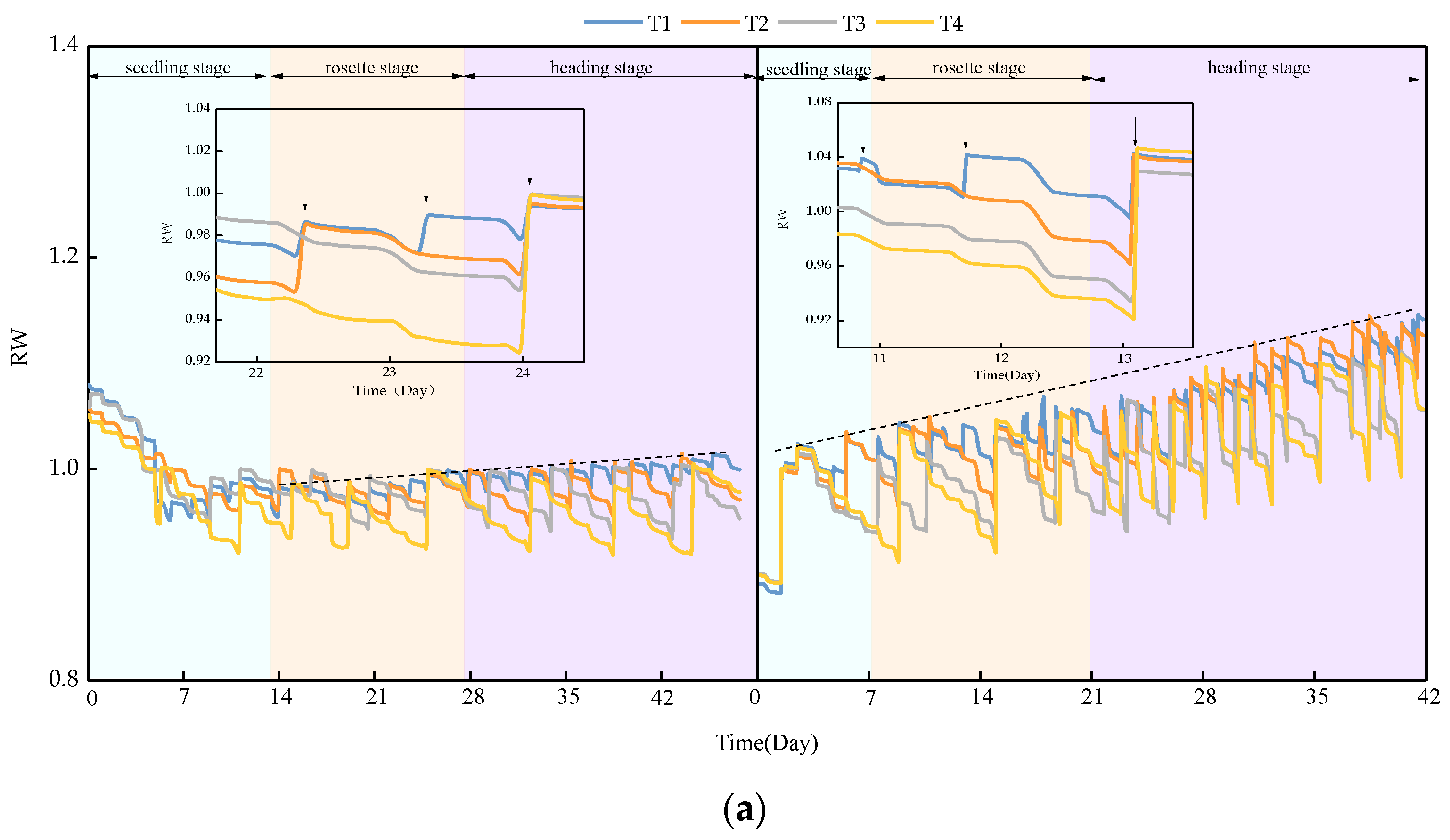
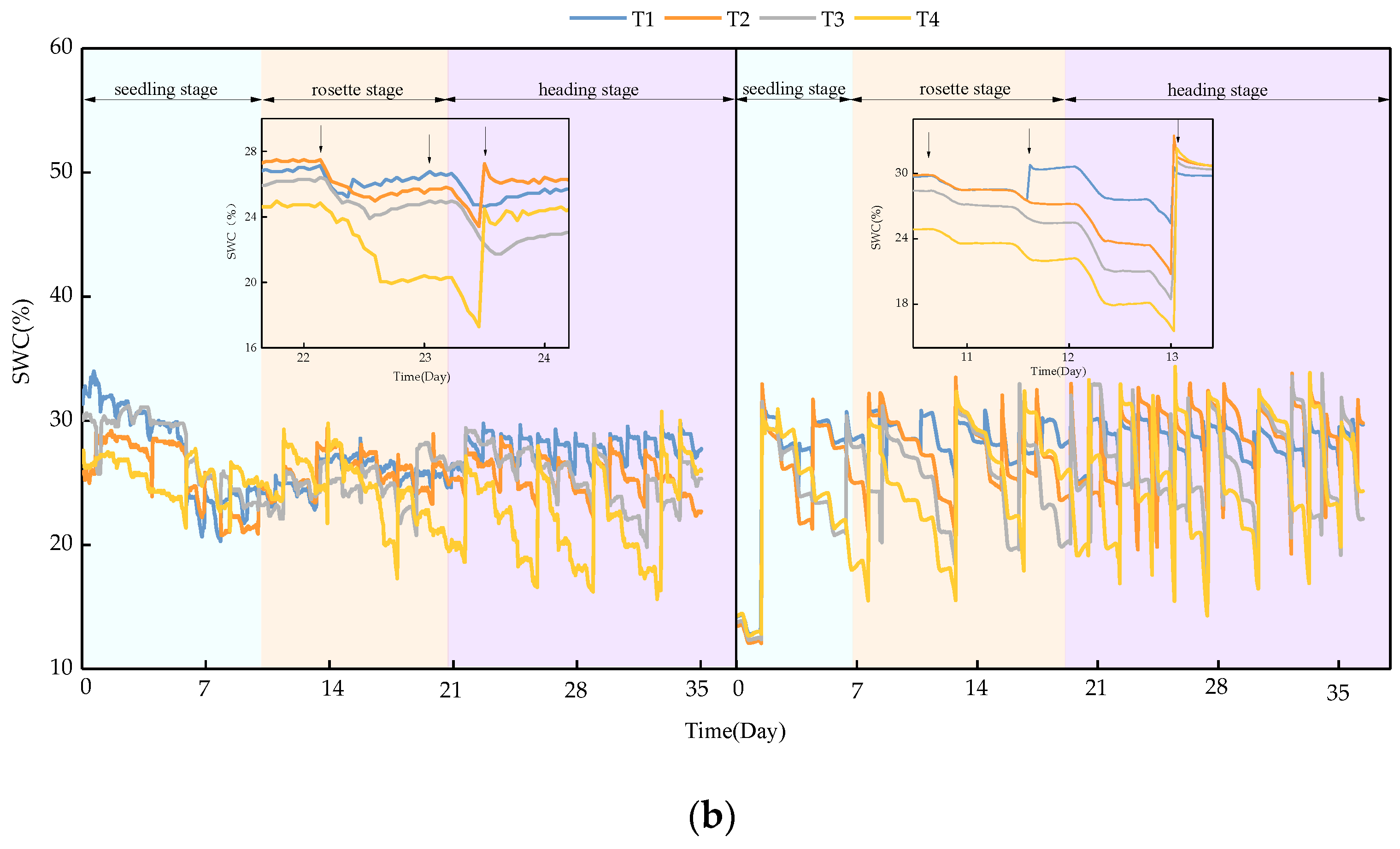
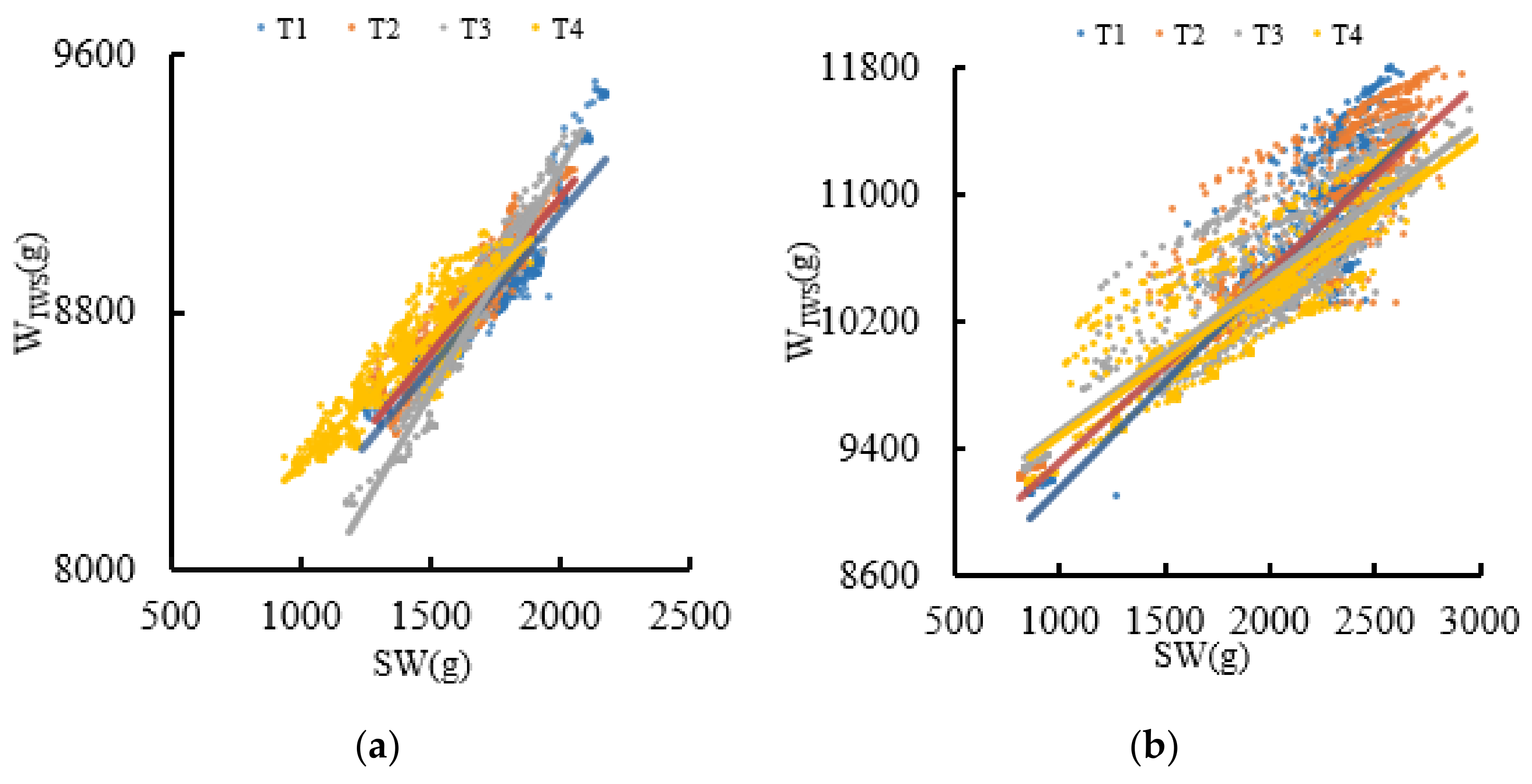
The IWS can sensitively reflect changes in crop weight during different growth periods at different times. The results indicate that WIWS and SWC have similar changing trends, and a significant correlation exists between WIWS and SW. The correlation in the second season is lower than that in the first season. This may be due to the different types of lettuce in the first and second seasons. The lettuce in the second season is three times as heavy as the lettuce in the first season. The daily weight gain of lettuce is ignored because it is small. However, under a similar SW, as the weight of the lettuce in the latter period increases, the variation range of WIWS is affected by the weight of the lettuce, resulting in scattered data and reduced correlation.
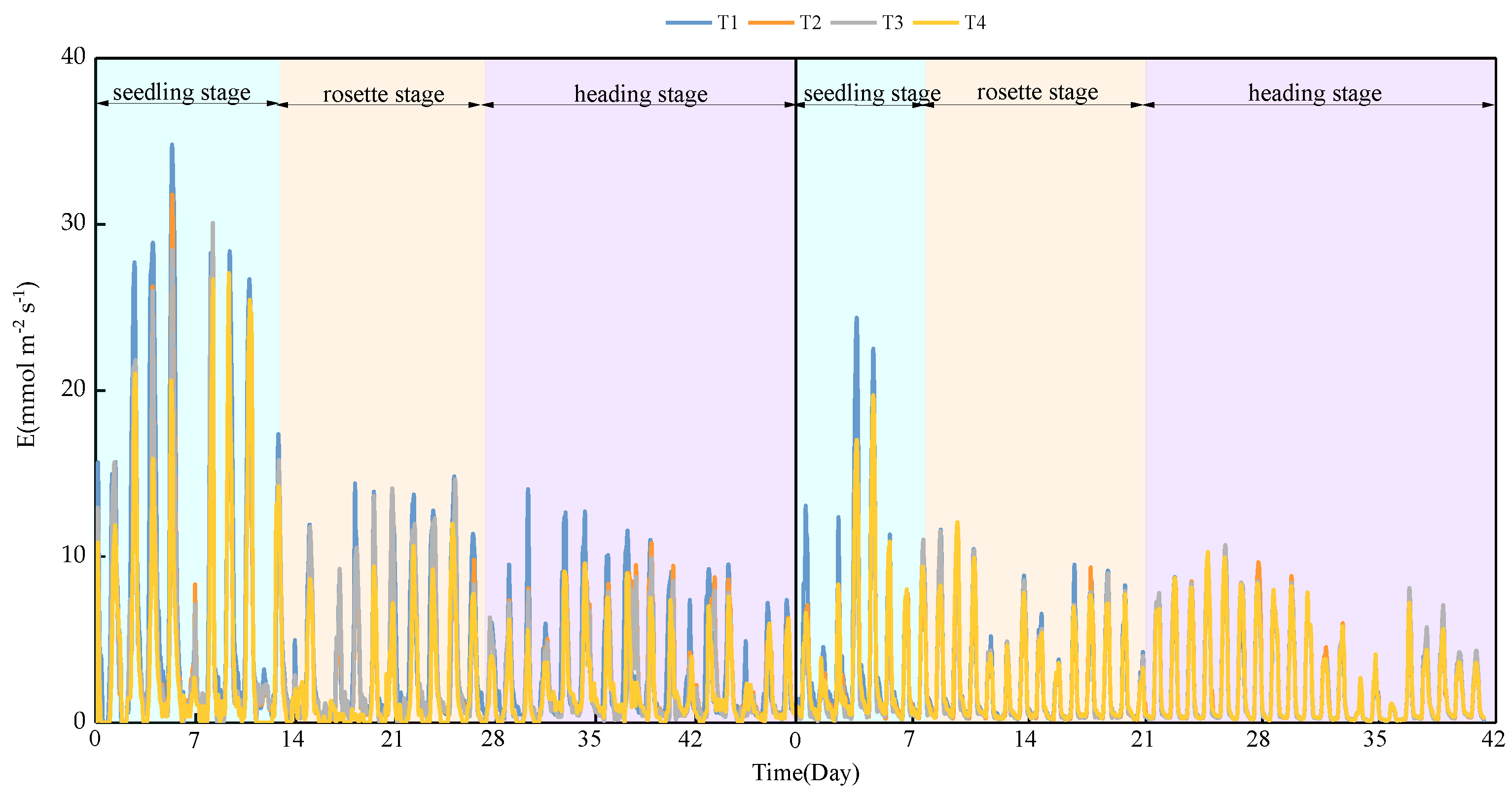
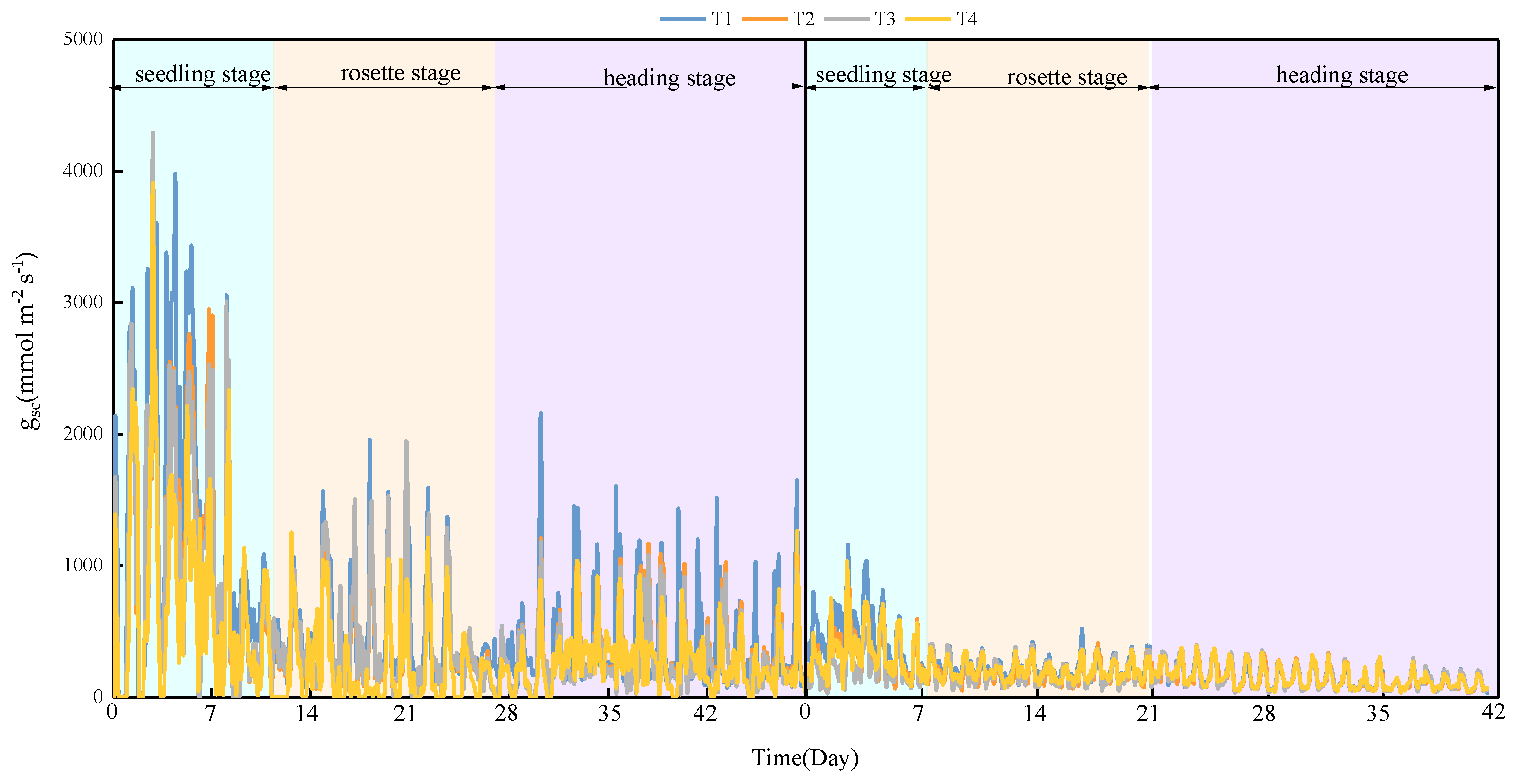
“E” refers to the amount of water transpired per unit leaf area of crops over a certain period of time. Plant water transpiration is mainly performed by the stomata of leaves, which is an important channel for the exchange of gas and water between leaves and the external environment. The opening and closing of stomata play an important role in plant transpiration. The results of the experiments indicate that as the irrigation volume decreases, E and gsc also decrease. Álvarez et al. [25] believe that deficit irrigation treatment reduces stomatal conductance, which reduces the relative growth rate of plants, as well as transpiration and photosynthesis. This is because when crops suffer from soil water deficit, they cannot obtain the water required to meet the photosynthesis of plants. The photosynthesis of plants is weakened, the gsc of crops will decrease, and E will also decrease, so as to effectively reduce the water loss of crops during transpiration. The E and gsc of lettuce under T2 treatment are higher than those under other water treatments when the lettuce enters into the rosette and heading stages. This is because the SWC under T1 treatment is too high, which inhibits lettuce respiration, thus affecting transpiration and photosynthesis. Under T4 treatment, the SWC is too low to meet the water required for photosynthesis in lettuce, and photosynthesis is weakened [26]. In addition, the leaf area of lettuce under T2 treatment is significantly higher than that of the other treatments, which increases the gsc of lettuce. In the first season, the leaf area under T1, T2, T3, and T4 treatments were 464.67 cm2, 481.64 cm2, 473.30 cm2, and 403.30 cm2, respectively. In the second season, the leaf area under T1, T2, T3, and T4 treatments were: 2515.50 cm2, 2609.63 cm2, 2104.87 cm2, and 1849.75 cm2, respectively.
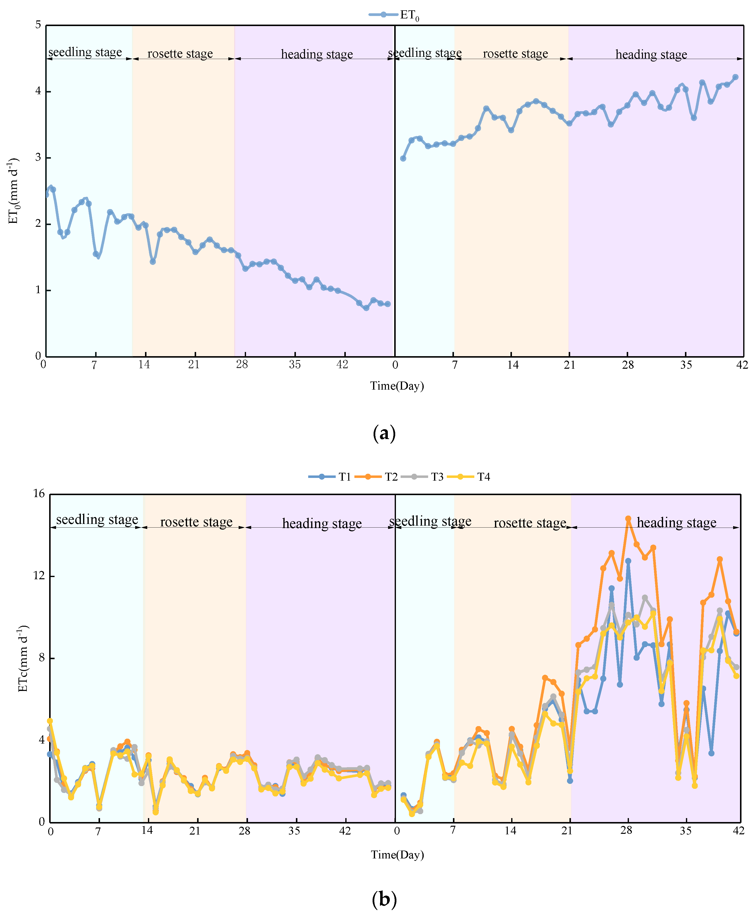
Based on the IWS, the weight of lettuce was monitored in real time and continuously, and the variation law of plant evapotranspiration during the growth period was analyzed. The change of ETc is closely related to the change of environmental factors; hence, we further explore the relationship between ETc and environment (Table 5). There is a significant positive correlation between ETc and T under different water treatments. With the increase of temperature, plant evapotranspiration also increases. The results of the first and second seasons indicate that the ETc and water consumption of the T2 treatment are higher than those of other treatments in the rosette and heading stages. This is because with the passage of time, the leaf area of plants under T2 treatment gradually increases and photosynthesis is gradually enhanced, resulting in an increase in the ETc of plants. This finding is similar to the results reported by Chang et al. [27].
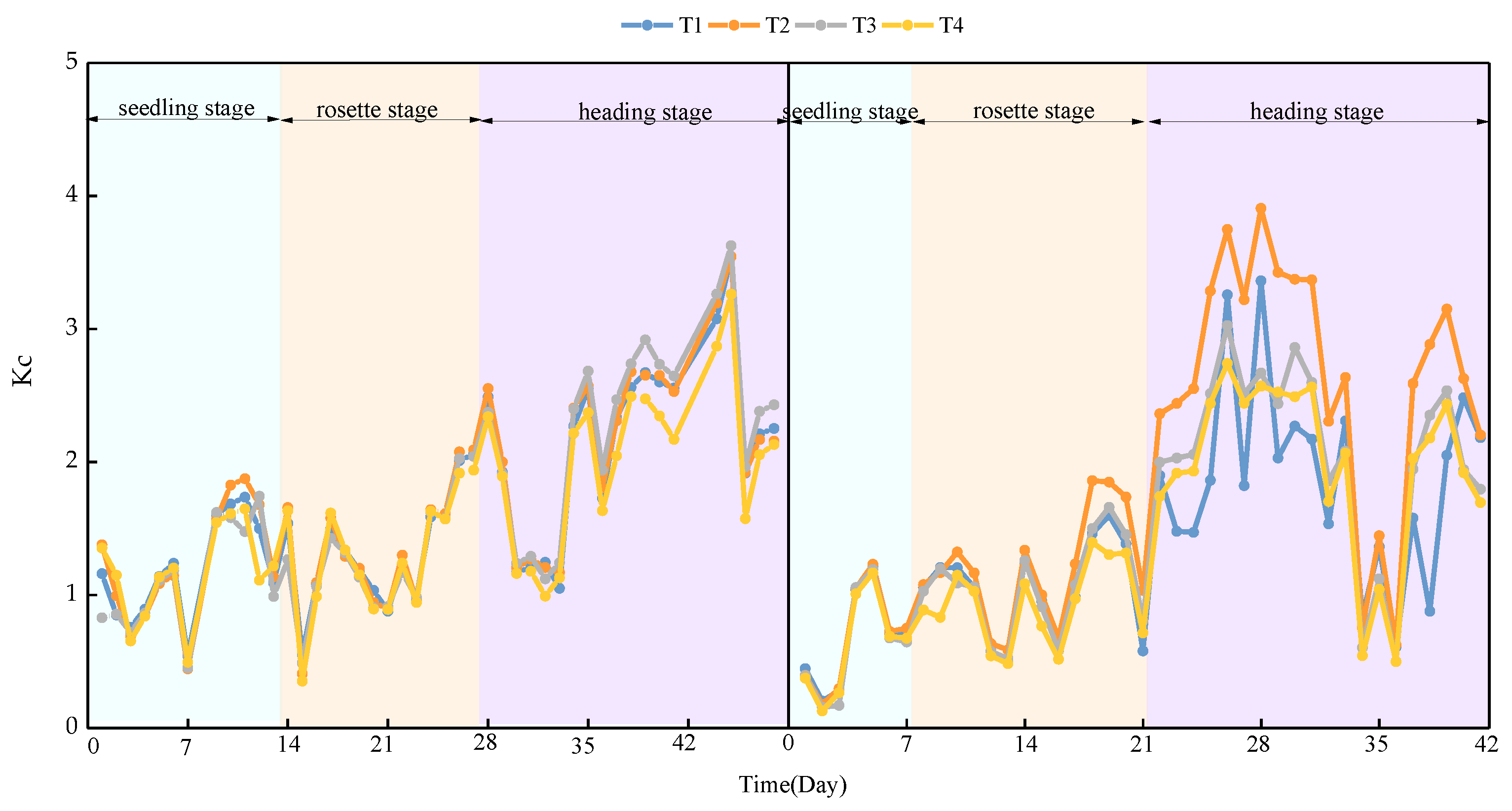
Water regulation has an important effect on plant growth and output. Kc is an important parameter for calculating crop ETc and reflects the influence of the biological characteristics of the crop itself, crop type, and yield level on crop water demand. Obtaining the Kc accurately is difficult. Currently, this process is mainly based on experience values [28,29,30]. This study analyzes the ETc of lettuce based on the IWS and calculates the ET0 through the environmental parameters obtained by the weather station to analyze the daily Kc of lettuce. Studies have indicated that under different water treatments, Kc decreases as the amount of irrigation decreases. This may be because the crops under T4 treatment have been in severe water deficit for a long time during the rosette and heading stages, which inhibits the growth of crops. In the rosette and heading stages, the Kc under T2 treatment is higher than that under the other treatments, because the leaf area gradually increases over time.
Table 6 indicates that the yield under T2 treatment has significantly increased by 11.55%, 5.72%, and 15.80% compared with other treatments in the first season. In the second season, the yield under T2 treatment has significantly increased by 9.59%, 39.18%, and 61.36% compared with other treatments. From the perspective of IWUE, the T2 treatment significantly increases by 11.07%, 0.91%, and 2.16% compared with other treatments in the first season. In the second season, the T2 treatment significantly increases by 21.05%, 9.89%, and 13.47% compared with other treatments. From the perspective of WUE, lettuce in the second season has significantly higher water use efficiency than in the first season. This result may be because of the high temperature of the greenhouse in the second season, which increased transpiration of the lettuce, and increased the water demand, resulting in a reduction in water loss from irrigation. From the perspective of plant physiological monitoring by the IWS, the higher photosynthetic rate of T2 treatment in the first and second seasons promoted plant growth. Based on the results of the first and second seasons, it can be seen that the lower limit of soil water irrigation for lettuce planting is 80%. A very high or very low water level is not good for growth and development. Excessive water irrigation will cause the soil to be in a state of water saturation for a long time, resulting in soil waterlogging, and thereby forming hypoxia deficit in the root system, which affects the growth above ground. At a very low irrigation level, the water in the soil will not reach the environment required for the growth of lettuce, thus forming soil water deficit and affecting its growth rate. This finding is consistent with the results of previous studies [31,32].
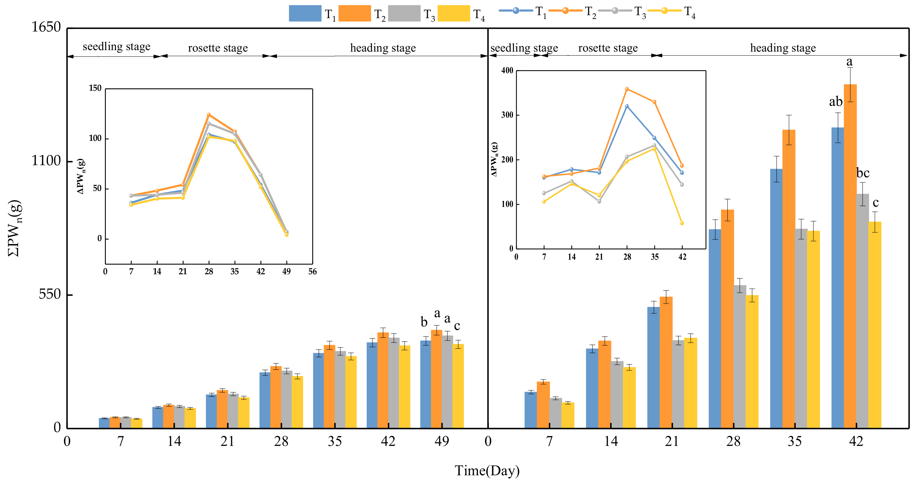
The results of growth physiological parameters of leaf-expansion lettuce in the first season and heading lettuce in the second season showed that the E and gsc of lettuce in the second season were lower than those in the first season. This was because the greenhouse temperature of lettuce in the heading stage in the second season was higher than that in the first season, which inhibited gsc and E. The ΔPWn of lettuce in the second season was faster than that in the first season, and the Kc and ETc of lettuce in the second season were higher than that in the first season. This is due to the different varieties and types of lettuce in the first season and the second season. The heading lettuce in the second season was heavier than the leaf-expansion lettuce in the first season, and the greenhouse temperature in the second season was higher, so the lettuce in the second season needed more water. However, the ΔPWn, E, gsc, yield, WUE, and other growth physiological parameters of lettuce in both of the first and second seasons were the highest under T2 treatment among the four different water treatments. The results show that T2 treatment has higher irrigation efficiency for different types of lettuce. Under the condition of water resource shortage, it can be used as a method for farmers to improve water use efficiency of lettuce.
The advantages of our IWS are as follows: 1. It can realize continuous online monitoring of SPAC, and the Kc analytical method is established. 2. It is not affected by soil texture. Currently, dielectric method is commonly used to measure soil moisture content [33]. Due to the complexity of the soil dielectric properties of different soil types, the high-precision measurement of soil moisture at different scales is affected in the measurement process. However, the IWS measures the changes of the entire soil. So, it would not be affected by the soil moisture accuracy measurement. 3. It is applicable to a wide range of plants, such as ornamental potted plants, leafy vegetables, flowers, etc. However, the application of IWS is also limited by specific crops. For crops such as tomatoes and cucumbers, vine hangings are required during the growth process. The hanging vines split the load with symmetrical weight, resulting in inaccurate measurements. Therefore, IWS can be improved and optimized by adding a plant-hanging scale in future research.

5. Conclusions

(1) During this study, an intelligent weighing system was used to realize real-time monitoring and analysis of soil moisture weight, weight gain, transpiration rate, stomatal conductance, evapotranspiration, and crop coefficients of potted lettuce. According to the online monitoring data of the intelligent weighing system, the changes in the soil-plant-atmosphere continuum at different times were reflected in real time. Simultaneously, the accuracy and feasibility of the data acquired through the intelligent weighing system were verified.
(2) Different water treatments had a significant impact on the soil-plant-atmosphere continuum of lettuce. Regarding soil, the relative system weight of the intelligent weighing system and the soil volumetric moisture content showed a consistent trend of increase and decrease, with a significant linear correlation (R2 = 0.639–0.941). Soil volumetric moisture content was higher under high moisture treatment, and the soil volumetric moisture content changed less. Regarding plants, the transpiration rate and stomata conductance of lettuce under the lowest water treatment in the first and second seasons were the lowest, which were 2.62 g·h−1 and 2.12 g·h−1, 364.60 mmol m−2 s−1 and 162.74 mmol m−2 s−1, respectively. In the atmospheric environment, with an increase in temperature, lettuce transpiration gradually increases. Under T2 treatment, the evapotranspiration of lettuce was 2.70%, 2.35%, 5.21% in the first season, and 32.07%, 23.21%, 31.05% in the second season, which was higher than that of the other treatments.
(3) An appropriate irrigation low limit could increase the yield of potted lettuce. Based on research results of the first and second seasons, the stomatal conductance, transpiration rate, weight gain, individual plant weight, and irrigation water use efficiency of lettuce all improved when the irrigation low limit was 80% field capacity. Moreover, the irrigation water use efficiency of lettuce under T2 treatment in the first and second seasons was significantly increased by 11.07%, 0.91%, 8.08%, and 21.05%, 9.89%, 13.47%, respectively, compared with the other treatments. The yields obtained were 0.425 kg and 1.428 kg, respectively.

Author Contributions

H.G., R.G. collected the meteorological data; H.G. analyzed the data; H.G. wrote the paper; R.G., Z.L. and X.Z. drew the figures for this paper; Z.L., H.G., H.Y., K.S., S.Z. and X.Z. reviewed and edited the paper. All authors have read and agreed to the published version of the manuscript.

Funding

The research was supported by the Key Research and Development Program of Yunnan (202002AE090010), the Innovation Ability Construction Project of Beijing Academy of Agriculture and Forestry Sciences (KJCX20200430 and KJCX20210402).

Institutional Review Board Statement

The authors declare that the study did not require ethical approval.

Informed Consent Statement

The authors declare that the study did not involve humans.

Data Availability Statement

The authors declare that the study did not report any data.

Conflicts of Interest

The authors declare no conflict of interest.

Nomenclature

AcronymMeaning of Words
SPACSoil-plant-atmosphere continuum
IWSIntelligent weighing system
KcCrop coefficient
SWCSoil volumetric moisture content
ET0Reference crop evapotranspiration
VPDVapor pressure deficit
WUEWater use efficiency
IWUEIrrigation water use efficiency
FCField capacity
WIWSIntelligent weighing system weight
SWSoil moisture weight
RWRatio of the weight at different times of the weighing to the initial weight
ΔPWnWeight gain change
gscStomatal conductance
ETcCrop evapotranspiration
ETranspiration rate

References

  1. Zhang, Z.; Huang, M. Effect of root-zone vertical soil moisture heterogeneity on water transport safety in soil-plant-atmosphere continuum in Robinia pseudoacacia. Agric. Water Manag. 2021, 246, 106702. [Google Scholar] [CrossRef]
  2. Che, C.; Zhang, M.; Argiriou, A.A.; Wang, S.; Du, Q.; Zhao, P.; Ma, Z. The Stable Isotopic Composition of Different Water Bodies at the Soil-Plant-Atmosphere Continuum (SPAC) of the Western Loess Plateau, China. Water 2019, 11, 1742. [Google Scholar] [CrossRef] [Green Version]
  3. Lei, G.; Zeng, W.; Jiang, Y.; Ao, C.; Wu, J.; Huang, J. Sensitivity analysis of the SWAP (Soil-Water-Atmosphere-Plant) model under different nitrogen applications and root distributions in saline soils. Pedosphere 2021, 31, 807–821. [Google Scholar] [CrossRef]
  4. García-Tejera, O.; López-Bernal, Á.; Testi, L.; Villalobos, F.J. Erratum to: A soil-plant-atmosphere continuum (SPAC) model for simulating tree transpiration with a soil multi-compartment solution. Plant Soil 2017, 418, 581. [Google Scholar] [CrossRef] [Green Version]
  5. Dainese, R.; Lopes, B.D.C.F.L.; Fourcaud, T.; Tarantino, A. Evaluation of instruments for monitoring the soil-plant continuum. Geomech. Energy Environ. 2021, 5, 100256. [Google Scholar] [CrossRef]
  6. Dardanelli, J.; Ritchie, J.; Calmon, M.; Andriani, J.; Collino, D. An empirical model for root water uptake. Field Crop. Res. 2004, 87, 59–71. [Google Scholar] [CrossRef]
  7. De Willigen, P.; van Dam, J.C.; Javaux, M.; Heinen, M. Root Water Uptake as Simulated by Three Soil Water Flow Models. Vadose Zone J. 2012, 11, vzj2012.0018. [Google Scholar] [CrossRef]
  8. Nagahage, E.A.A.D.; Nagahage, I.S.P.; Fujino, T. Calibration and Validation of a Low-Cost Capacitive Moisture Sensor to Integrate the Automated Soil Moisture Monitoring System. Agriculture 2019, 9, 141. [Google Scholar] [CrossRef] [Green Version]
  9. Shen, X.; Liang, J.; Zeleke, K.T.; Liang, Y.; Wang, G.; Duan, A.; Mi, Z.; Ning, H.; Gao, Y.; Zhang, J. Optimizing the Positioning of Soil Moisture Monitoring Sensors in Winter Wheat Fields. Water 2018, 10, 1707. [Google Scholar] [CrossRef] [Green Version]
  10. Getzin, S.; Erickson, T.E.; Yizhaq, H.; Muñoz-Rojas, M.; Huth, A.; Wiegand, K. Bridging ecology and physics: Australian fairy circles regenerate following model assumptions on ecohydrological feedbacks. J. Ecol. 2021, 109, 399–416. [Google Scholar] [CrossRef]
  11. Meloni, D.A.; Oliva, M.A.; Martinez, C.A.; Cambraia, J. Photosynthesis and activity of superoxide dismutase, peroxidase and glutathione reductase in cotton under salt stress. Environ. Exp. Bot. 2003, 49, 69–76. [Google Scholar] [CrossRef]
  12. Buczek, J.; Migut, D.; Jańczak-Pieniążek, M. Effect of Soil Tillage Practice on Photosynthesis, Grain Yield and Quality of Hybrid Winter Wheat. Agriculture 2021, 11, 479. [Google Scholar] [CrossRef]
  13. Álvarez, S.; Martín, H.; Barajas, E.; Rubio, J.A.; Vivaldi, G.A. Rootstock Effects on Water Relations of Young Almond Trees (cv. Soleta) When Subjected to Water Stress and Rehydration. Water 2020, 12, 3319. [Google Scholar] [CrossRef]
  14. Liu, C.; Cui, N.; Gong, D.; Hu, X.; Feng, Y. Evaluation of seasonal evapotranspiration of winter wheat in humid region of East China using large-weighted lysimeter and three models. J. Hydrol. 2020, 590, 125388. [Google Scholar] [CrossRef]
  15. Wang, T.; Melton, F.S.; Pôças, I.; Johnson, L.F.; Thao, T.; Post, K.; Cassel-Sharma, F. Evaluation of crop coefficient and evapotranspiration data for sugar beets from landsat surface reflectances using micrometeorological measurements and weighing lysimetry. Agric. Water Manag. 2021, 244, 106533. [Google Scholar] [CrossRef]
  16. Tyagi, N.; Sharma, D.; Luthra, S. Determination of evapotranspiration and crop coefficients of rice and sunflower with lysimeter. Agric. Water Manag. 2000, 45, 41–54. [Google Scholar] [CrossRef]
  17. Zheng, Y.; Zhao, Q.; Zhang, X.; Xue, X.; Zhong, Z.; Wang, S. Development of a multi-channel pot plant evapotranspiration measurement system based on LORA wireless technology. Water Sav. Irrig. 2020, 3, 77–84. [Google Scholar]
  18. Wang, X.; Wu, Y.; Zhang, Z.; Guo, R.; Wang, L. Effects of magnetization treatment of different water sources on photosynthesis, mineral elements and yield of lettuce. J. Irrig. Drain. 2021, 40, 40–47. [Google Scholar]
  19. Wilcox, J.C. Rate of soil drainage following an irrigation: III. A new concept of the upper limit of available moisture. Can. J. Soil Sci. 1962, 42, 122–128. [Google Scholar] [CrossRef]
  20. GB/T 50485-2009; Technical Specification for Micro-Irrigation Engineering. SAC: Beijing, China, 2009; Volume 12.
  21. Liao, R.; Zhang, S.; Zhang, X.; Wang, M.; Wu, H.; Zhangzhong, L. Development of smart irrigation systems based on real-time soil moisture data in a greenhouse: Proof of concept. Agric. Water Manag. 2021, 245, 106632. [Google Scholar] [CrossRef]
  22. Zhang, F.; Liu, Z.; Zhangzhong, L.; Yu, J.; Shi, K.; Yao, L. Spatiotemporal Distribution Characteristics of Reference Evapotranspiration in Shandong Province from 1980 to 2019. Water 2020, 12, 3495. [Google Scholar] [CrossRef]
  23. Halperin, O.; Gebre, A.; Wallach, R.; Moshelion, M. High-throughput physiological phenotyping and screening system for the characterization of plant-environment interactions. Plant J. 2017, 89, 839–850. [Google Scholar] [CrossRef] [PubMed]
  24. González-Esquiva, J.; Oates, M.; García-Mateos, G.; Moros-Valle, B.; Martínez, J.M.M.; Ruiz-Canales, A. Development of a visual monitoring system for water balance estimation of horticultural crops using low cost cameras. Comput. Electron. Agric. 2017, 141, 15–26. [Google Scholar] [CrossRef]
  25. Álvarez, S.; Sánchez-Blanco, M.J. Changes in growth rate, root morphology and water use efficiency of potted Callistemon citrinus plants in response to different levels of water deficit. Sci. Hortic. 2013, 156, 54–62. [Google Scholar] [CrossRef] [Green Version]
  26. Sánchez-Blanco, M.J.; Álvarez, S.; Navarro, A.; Bañón, S. Changes in leaf water relations, gas exchange, growth and flowering quality in potted geranium plants irrigated with different water regimes. J. Plant Physiol. 2009, 166, 467–476. [Google Scholar] [CrossRef] [Green Version]
  27. Chang, X.; Zhao, W.; Zhao, A.J. Dynamics of leaf area index and its relationship with water consumption of Populus chinensis in the middle reaches of heihe River. Glaciol. Geocryol. 2006, 1, 85–90. [Google Scholar]
  28. Irmak, S.; Irmak, A.; Allen, R.; Jones, A.J. Solar and net radiation-based equations to estimate reference evapotranspiration in humid climates. J. Irrig. Drain. Eng. 2003, 129, 336–347. [Google Scholar] [CrossRef]
  29. Pereira, L.; Paredes, P.; López-Urrea, R.; Hunsaker, D.; Mota, M.; Shad, Z.M. Standard single and basal crop coefficients for vegetable crops, an update of FAO56 crop water requirements approach. Agric. Water Manag. 2021, 243, 106196. [Google Scholar] [CrossRef]
  30. Saitta, D.; Vanella, D.; Ramírez-Cuesta, J.M.; Longo-Minnolo, G.; Ferlito, F.; Consoli, S. Comparison of Orange Orchard Evapotranspiration by Eddy Covariance, Sap Flow, and FAO-56 Methods under Different Irrigation Strategies. J. Irrig. Drain. Eng. 2020, 146, 05020002. [Google Scholar] [CrossRef]
  31. Fan, Y.; Massey, R.; Park, S.C. Multi-Crop Production Decisions and Economic Irrigation Water Use Efficiency: The Effects of Water Costs, Pressure Irrigation Adoption, and Climatic Determinants. Water 2018, 10, 1637. [Google Scholar] [CrossRef] [Green Version]
  32. Liu, Y.; Li, S.; Chen, F.; Yang, S.; Chen, X. Soil water dynamics and water use efficiency in spring maize (Zea mays L.) fields subjected to different water management practices on the Loess Plateau, China. Agric. Water Manag. 2010, 97, 769–775. [Google Scholar] [CrossRef]
  33. Bobrov, P.P.; Belyaeva, T.A.; Kroshka, E.S.; Rodionova, O.V. Soil Moisture Measurement by the Dielectric Method. Eurasian Soil Sci. 2019, 52, 822–833. [Google Scholar] [CrossRef]
Figure 1. Irrigation amount and irrigation time (a) irrigation amount and irrigation time for planting lettuce in the first season, (b) irrigation amount and irrigation time for planting lettuce in the second season.
Water 14 00673 g001
Figure 2. Test layout (a) first season, (b) second season.
Water 14 00673 g002
Figure 3. Technology roadmap.
Water 14 00673 g003
Figure 4. Hardware structure diagram of IWS.
Water 14 00673 g004
Figure 5. Changes of RW and SWC under different water treatments (a) RW change of lettuce in the first and second seasons under different water treatments, (b) SWC change under different water treatments in the first and second seasons.
Water 14 00673 g005aWater 14 00673 g005b
Figure 6. The fitting of SW and WIWS under different water treatments. (a) First season, (b) second season.
Water 14 00673 g006
Figure 7. Changes of lettuce weight under different water treatments. Note: The bars with different letters showed significant difference (α = 0.05). The same as below.
Water 14 00673 g007
Figure 8. E changes under different water treatments.
Water 14 00673 g008
Figure 9. gsc changes under different water treatments.
Water 14 00673 g009
Figure 10. Changes of photosynthetic parameters of lettuce leaves in one day under different water treatments; (a) measured value and test value of E; (b) measured and experimental values of gsc.
Water 14 00673 g010
Figure 11. ET0 and ETc changes under different water treatments (a) ET0, (b) ETc.
Water 14 00673 g011
Figure 12. Kc changes under different water treatments.
Water 14 00673 g012
Table 1. Irrigation treatment design.
TreatmentPlanting SeasonT1T2T3T4
Irrigation maximums 100% FC
Irrigation minimums90% FC80% FC70% FC60% FC
Irrigation
amount/mm
First season116.21112.04109.35105.16
Second season254.15235.84202.94172.23
Table 2. Regression analysis of SW and WIWS under different water treatments.
Planting SeasonTreatmentFitted EquationDetermination Coefficient/R2p
First seasonT1WIWS = 0.96 SW + 7186.50.87**
T2WIWS = 0.96 SW + 7226.40.87**
T3WIWS = 1.39 SW + 6472.00.94**
T4WIWS = 0.79 SW + 7541.20.85**
Second seasonT1WIWS = 1.33 SW + 7830.10.64**
T2WIWS = 1.21 SW + 8094.30.73**
T3WIWS = 0.97 SW + 8525.90.70**
T4WIWS = 0.95 SW + 8534.40.76**
Note: ** means the difference between the two variables is extremely significant.
Table 3. Analysis of univariate variance for different water treatments.
Planting Season Quadratic SumDegree of FreedomMean SquareFSignificant
First Season Among groups6500.9232166.9746.600.00
Group communication372.00846.50
Gross6872.9211
Second seasonAmong groups556,997.083185,665.696.5740.02
Group communication225,944.99828,243.12
Gross782,942.0711
Table 4. Kc and water consumption of lettuce.
IndexPlanting SeasonTreatmentGrowth Period
Seedling StageRosette StageHeading Stage
Crop coefficientsFirst seasonT11.10 a1.26 a2.17 a
T21.11 a1.28 a2.20 a
T31.02 b1.21 a2.26 a
T41.11 a1.21 a2.01 b
Second seasonT10.65 a1.01 a2.35 b
T20.65 a1.16 b2.65 a
T30.61 a1.02 a2.07 c
T40.61 a0.91 a1.97 cd
Water consumption rateFirst seasonT12.36 a2.31 a2.40 a
T22.39 a2.37 a2.45 a
T32.19 b2.21 a2.50 a
T42.39 a2.23 a2.24 b
Second seasonT11.17 a4.52 a8.96 a
T22.37 b4.39 b8.22 b
T30.75 c3.86 c8.14 b
T40.70 c3.68 c7.37 c
Water consumption modulus/%First seasonT119.99 b32.57 ab47.45 b
T219.85 b32.76 ab47.39 b
T318.75 a31.48 b49.77 c
T421.10 c32.81 a46.09 a
Second seasonT12.75 a26.71 a70.54 b
T25.82 b26.95 a67.23 c
T31.66 c25.82 b72.52 a
T41.70 c26.81 a71.49 b
Note: The values with different letters indicate significant differences between different water treatments (p < 0.05).
Table 5. Correlation analysis between ETc and temperature.
Planting SeasonETcρ
First seasonT10.854 **
T20.916 **
T30.798 **
T40.882 **
Second seasonT10.816 **
T20.829 **
T30.799 **
T40.807 **
Note: ** means very significant (p < 0.01).
Table 6. Analysis of lettuce weight and water use efficiency under different water treatments.
Planting SeasonTreatmentYield/(kg)IWUE/(kg/m3)WUE/(g/kg)
First season T10.381 b48.67 ab56.27 b
T20.425 a54.06 a61.34 a
T30.402 a53.57 ab59.42 a
T40.367 c50.02 b55.88 b
Second seasonT11.303 ab65.42 a83.26 b
T21.428 a79.19 bc94.88 a
T31.026 bc72.06 c74.21 c
T40.885 c69.79 a69.74 c
Note: The values with different letters indicate significant differences between different water treatments (p < 0.05).
Publisher’s Note: MDPI stays neutral with regard to jurisdictional claims in published maps and institutional affiliations.

