Hydrogeomorphic Scaling and Ecohydraulics for Designing Rescaled Channel and Floodplain Geometry in Regulated Gravel–Cobble Bed Rivers for Pacific Salmon Habitat

Abstract

Societies are increasingly restoring and/or rehabilitating rivers below dams for keystone species such as salmon. A fundamental concept for rehabilitating river morphology below dams for salmon is that a rescaled version of the river corridor synchronized to the regulated flow regime can restore habitat quantity and quality. Downscaled and resized hydrographs have been shown to provide environmental benefits to fish communities including salmon as well as riparian vegetation communities. However, less research exists on how this can be achieved through the topographic rescaling of heavily modified and regulated river corridors. The goal of this paper is to review analytical methods to determine initial of size of rescaled channel and floodplain mesohabitat units in regulated gravel–cobble bed rivers for Pacific salmon (Oncorhynchus spp.) habitat using hydrogeomorphic scaling and ecohydraulics. Hydrogeomorphic flow scaling is the prediction of river morphology and geometry using empirical and analytical relationships. Ecohydraulic scaling refers to the use of ecohydrology, habitat suitability curves, and fish density relationships to determine the size of mesohabitat units for ecologically relevant flows. In practice, these are complimentary first order estimates of channel and floodplain configurations followed by iterative design in a hierarchical manner. This review advances the science of river design by synthesizing these complimentary ideologies for Pacific salmon habitat restoration in regulated rivers. Following the review, the layout of features is briefly discussed followed by a discussion of important considerations beyond the physical and topographic rescaling of river corridors for salmonid habitat restoration.

1. Introduction

Environmental degradation and shifting societal values have led to widespread restoration of rivers and streams below dams [1,2,3,4,5,6,7,8]. Herein the term restoration is used as an accepted colloquial term to refer to naturalization, enhancement and rehabilitation of rivers and streams [4]. Restoration can apply to generic ecosystem services or specific flora and fauna, but here I focus on Pacific salmon of the genus Oncorhynchus, which have a high ecological, cultural and economic value [9] (Figure 1). Dam construction and flow regulation in gravel–cobble bedded rivers can alter sediment supply and flow regime which can channelize and simplify alluvial river morphology through channel bed incision, armoring and riparian vegetation encroachment [10,11,12,13]. Further, development of historic floodplains for agriculture, urban expansion and mining modifies the form and function of river corridors [14,15]. Together, flow regulation and floodplain development can greatly affect Pacific salmon spawning and rearing habitat with population level consequences [16].

One can simplify the diversity of approaches to Pacific salmon habitat restoration below dams as altering flow, form and/or sediment supply [8,18,19,20]. Alterations to flow include the prescription of hydrographs to support ecosystem function or specific habitat needs [21,22], while alteration of form includes the addition of instream structures [23] and channel and floodplain manipulation that aims to recontour the river corridor [24,25,26,27,28]. Sediment supply is addressed less often through the augmentation of sediment, generally coarse sediment for salmon spawning [3,29,30,31]. Flow regime and channel and floodplain manipulation are not independent of each other, but are complimentary actions needed to improve riverine habitat for salmon [8].

Returning rivers to prior or historical conditions is not a feasible alternative when hydrologic inputs and river corridor extents have been significantly modified. Rather, fluvial systems should be designed for present inputs while factoring in anticipated future conditions related to climate change or management [32]. A fundamental concept for rehabilitating river corridors below dams for salmon is that a rescaled version of the river corridor synchronized to the regulated flow regime can restore habitat quantity and quality [1]. Downscaled and resized hydrographs have been shown to provide environmental benefits to fish communities including salmon [33,34] as well as riparian vegetation communities [22]. Topographic rescaling of river channels entails spawning riffle, gravel bar, and pool creation [35,36] as well as the manipulation of off-channel and floodplain features to create juvenile rearing habitat for post-dam flow regimes [28,37]. For example, in the gravel–cobble bedded reaches of California’s Merced River below Crocker-Huffman Dam there have been over 6 km of river channel and off-channel habitats restored for fall-run Chinook salmon (Oncorhynchus tshawytscha) using the concept of rescaling the river channel to remediate impacts from flow regulation and gravel and sand mining (Figure 2). While it has been demonstrated that rescaling river channels below dams can improve salmonid habitat [38,39], few studies have discussed how to design these features within the template of regulated and highly modified river corridors.

Modern river restoration design proceeds hierarchically and relies heavily on numerical modeling to evaluate scenarios prior to implementation. Hierarchical design implies that the process of developing and evaluating scenarios is layered, and many examples exist in the literature [3,40,41,42]. Goals are developed, baseline data is collected and depending on existing conditions and site constraints [35,43], concepts and river design scenarios are developed, evaluated, and iterated upon. The Spawning Habitat Integrated Rehabilitation Approach (SHIRA; [3,44]) lays out a framework for the design of spawning riffles in regulated rivers below dams where gravel augmentation is the primary physical action, and this approach has been heavily vetted with much success [25,45,46,47]. Ample literature exists describing how river design scenarios can be created [48] as well as how ecohydraulic and sediment transport modeling can be used to evaluate and refine designs for salmonid habitat, especially spawning [3,24,43]. It is also becoming more common to model and assess geomorphic and ecological processes [41,49,50,51]. Moreover, morphodynamic modeling can be used to evaluate designs beyond their initial condition to assess potential evolutionary trajectories of river morphology and physical habitat [52,53,54].

Despite the above advances, there are areas that could be improved to help advance the science of river design [6] for Pacific salmon habitat in regulated rivers. It is not clear how to objectively inform the development of river design scenarios beyond simple hydraulic engineering constructs such as stable channel design, expert opinion, and artistry. There are many ways to create designs for river restoration projects [48], but many methods are very rarely used, with a long standing use of computer assisted drafting programs. Synthetic river channel design has helped show how to create artificial terrains with variability associated with specific form–process linkages thought to benefit Pacific salmon [41], but there is a gap in how to embed those concepts in actual real word river corridors. Further, questions such as why certain mesohabitat units are located in specific areas never get asked until the features are created and fail relative to goals [55,56]. The above considerations are important because the initial conditions of all fluvial systems have a strong influence on their evolutionary trajectory [57]. Given the social and financial barriers to restoring rivers and streams, there is thus great value in developing a river corridor design that leverages what we know about river form and process and habitat for aquatic organisms.

The goal of this paper is to review analytical methods to determine initial of size of rescaled channel and floodplain mesohabitat units in regulated gravel–cobble bed rivers for Pacific salmon habitat using hydrogeomorphic scaling and ecohydraulics (Figure 3). Hydrogeomorphic flow scaling is the prediction of river morphology and geometry using empirical and analytical relationships. Ecohydraulic scaling refers to the use of ecohydrology, habitat suitability curves, and fish density relationships to determine the size of mesohabitat units for ecologically relevant flows. They represent a needed duality where hydrogeomorphic scaling is concerned with physical science (i.e., fluvial geomorphic) aspects of river restoration, while ecohydraulic scaling is meant to place those aspects in context with the physical habitat needs of aquatic organisms such as Pacific salmon. In practice, these are complimentary and necessary first order estimates of channel and floodplain configurations followed by iterative design in a hierarchical manner (Figure 3) [3,39,40].

Clarification is needed for the use of the term mesohabitat units and the applicability of these concepts. Mesohabitat units are by definition areas that represent physical conditions including river morphology (i.e., riffle, pool, and bar), specific habitat associations, and processes needed to maintain these features [58]. The term geomorphic unit is not used because those features are commonly concerned with areas formed under a specific set of geomorphic processes and do not usually consider habitat [59]. The concepts presented herein focus on Pacific salmon and throughout the paper an example is used for native fall-run Chinook salmon (Oncorhynchus tshawytscha) in the regulated and highly modified Merced River located in the Central Valley of California, USA. Background for Chinook salmon habitat restoration in the Merced River can be found in [34,35,37,59].

This review advances the science of river design by synthesizing the complimentary ideologies of hydrogeomorphic and ecohydraulic scaling for Pacific salmon habitat restoration in regulated rivers. Critiques of river restoration often lament that the paradigm is driven by ideals of stable and static river channels, and that biological aspects need to be included on par with physical science and engineering considerations [5]. Broad reviews that call for the integration of natural geomorphic process and biological considerations [60] often do not provide the detail to design rivers in regulated and managed river corridors. In these settings it not possible to remove every stressor and address all catchment scale problems, but there is nonetheless an opportunity to improve rivers and streams for Pacific salmon. While prior work has highlighted how a mesohabitat unit approach utilizing ecohydraulics could be used in stream restoration [58], there are no studies on how to determine the type, size, and location of these features. In the below subsections these two approaches are reviewed followed by how this information can help inform the layout of geomorphic and mesohabitat unit designs. I close with a discussion of other important considerations beyond the initial rescaling of river corridors for Pacific salmonid habitat restoration.

2. Hydrogeomorphic Scaling

Basic hydrogeomorphic relationships blend analytical and empirical theory. Early on these relationships were strictly empirical [61,62], but more recently they have taken the form of analytical treatments of reach scale hydraulic and sediment transport theory [63,64,65]. Purely empirical approaches usually define a channel geometry or morphologic attribute as a function of discharge or mean channel width [61,66,67]. Theoretical treatments involve invoking relationships of open channel flow and sediment transport with empirical relationships that provide closure to the inherently indeterminate nature of river form [68]. The general sequence of hydrogeomorphic scaling is to select scaling variables, such as a representative channel forming flow, sediment size and valley gradient, which are then used to estimate a reach-averaged bankfull width and depth (Figure 3). These are then used to predict the planform typology and geometry, as well as bedform and floodplain scaling. Variability in riffle, bar and pool units can also be embedded to support hydrogeomorphic processes.

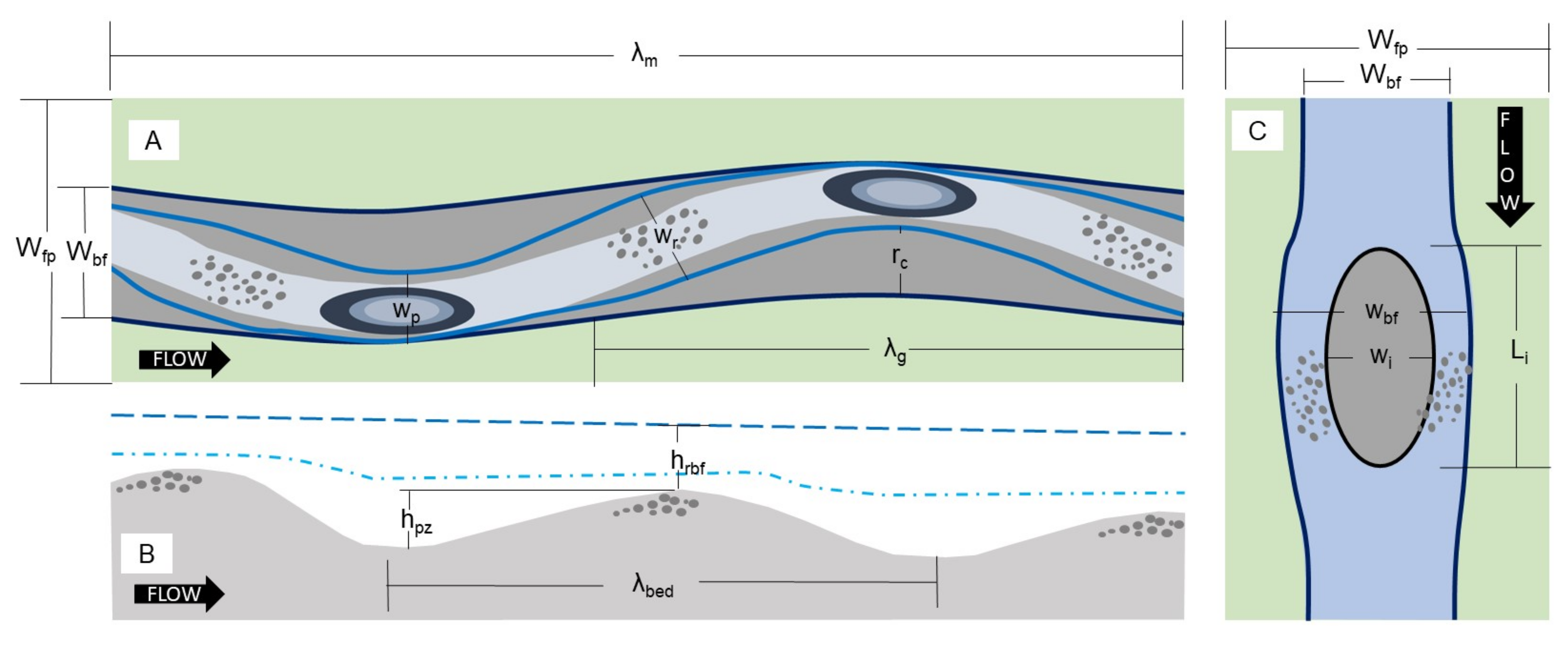
2.1. Scaling Variables

Scaling variables needed to predict alluvial river channel morphology include at a minimum reach averaged values of slope ($S$), median sediment size ($D_{50}$) and a representative channel forming or bankfull flow $\left(Q_{bf}\right)$. There exist different ways of calculating a channel forming discharge including using the mean annual flood, bankfull discharge, or effective discharge [40,69]. Nonetheless, in this paper we use the bankfull terminology because it has become ingrained the description of alluvial channel form. While one can of course calculate bankfull discharge based on flow records using assumed flow frequencies such as the 1.5–5-year flood events, this may be incorrect for regulated and disturbed rivers that are the focus of restoration. Rivers with flow regulation usually have alterations to hydrology and channel form that may sever the linkages between flow and form that give the bankfull concept value [12,70]. Further, the bankfull concept was derived in humid, sub-tropical climates in the Eastern United States, and its validity in Mediterranean climates such as the Central Valley of California, USA, has been questioned since these rivers have highly variable flow regimes [2]. Effective discharge analyses are preferred over return interval or bankfull approaches because the use of cumulative sediment discharge curves allow quantification of the sediment budget relative to the hydrologic regime [69]. Lastly, one should consider that flow regimes in regulated rivers are often controlled by regulatory statues that require minimum seasonal flows and pulse flows for specific ecological needs, as well as limits to flood magnitude from the capacity of the adjacent and/or downstream flood control system [33,34,70,71,72]. Seasonal pulse flows for fish attraction, rearing and outmigration are generally well constrained in terms of magnitude and duration [71,73]. Similarly, peak winter flows are also generally constrained to the rating of downstream levees [74,75].

Grain size, usually represented as the median sediment size $(D_{50})$, is a fundamental attribute of alluvial river morphology [76]. Pacific salmon have biophysical limits on their ability construct redds and reproduce [73,74]. Thus, an important aspect of channel sizing is the explicit consideration of sediment sizes needed to accommodate salmonid spawning and incubation [29,72,73]. Many river restoration projects below dams use gravel augmentation using a sediment gradation specifically tailored to spawning salmon and/or optimize spawning and embryo survival [30,77]. This can be incorporated by using a $D_{50}$ or $D_{84}$ that is commensurate with the grain size distribution fish can mobilize for redd construction. Spawning gravel estimates can be generated from using a simple rule that the $D_{50}$ equates to 10% the average body length of adult fish [78]. Riebe et al. [77] build on this work by developing a way to evaluate the effect of the $D_{50}$ and $D_{84}$ on the number of redds a substrate can accommodate. If all one knows is the $D_{50}$ the Fuller and Thompson relationship [79] can be used to model a natural sediment gradation. The relationship takes the form:

$$P=100\left[{\left(d/D_{max}\right)}^n\right]$$

(1)

where $P$ is the percentage of the mixture smaller than $d$, $D_{max}$ is the largest material in the mixture, and $n$ is a parameter that ranges to determine how fine or coarse the mixture is. When $n=0.5$ it produces a maximum density mixture when particles are round.

The gradient or slope of a river controls the rate at which potential energy of river flow is dissipated and is thus a fundamental scaling variable for determining alluvial channel geometry [65,80]. Studies suggest that most gravel and cobble bed reaches below dams adjust their gradient and geometry relatively quickly, within <50 years [81], but every river is unique. Dade [82] and Grant [13] offer quantitative frameworks for predicting the extent of possible adjustment of gravel and cobble bed rivers below dams. There are two end-member choices for selecting a design slope in this context (Figure 4). First, one can assume that the riverbed profile has equilibrated from flow regulation, in which case the current valley or reach slope can be used (Figure 4, case 1). Second, one can determine a new slope based on the channel geometry and grain size for rescaled conditions, explicitly accounting for sediment transport needed to maintain the new gradient (Figure 4, case 2). This concept of “slope creation” was studied by Elkins et al. [25] in the context of gravel augmentation immediately below a dam where riffle to riffle slope is increased by adding elevation to created or enhanced riffles. Importantly, when creating slope there usually needs to be an explicit increase in sediment supply through gravel augmentation to maintain the newly imposed slope. In either case there is usually a “tie-in” riffle or feature at the downstream end of the reach that the selected gradient is extrapolated from, which allows bed elevations to be approximated.

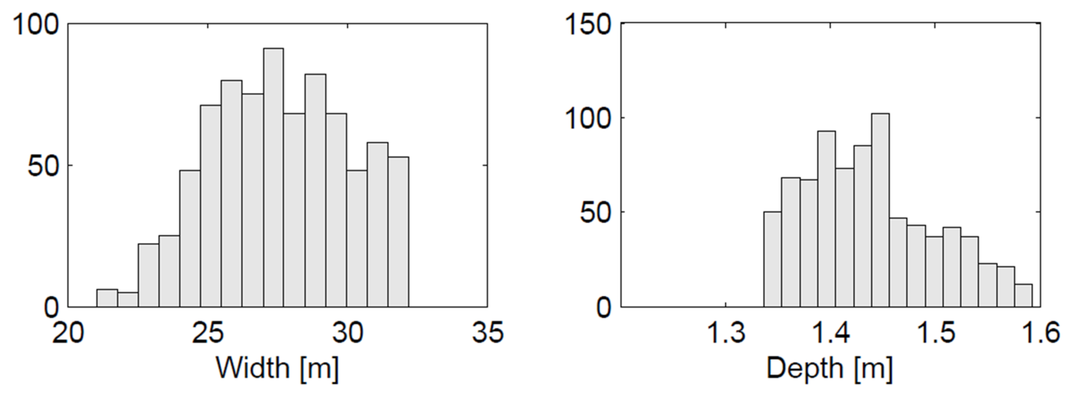
2.2. Channel Geometry

River geometry and associated flow characteristics are inherently indeterminate [68], and as a result there have been purely empirical, analytical and hybrid attempts at scaling relationships to determine the width and depth of river channels. There is an immense amount of literature concerning this topic [78,79,80,81,82,83,84,85,86,87,88,89], but the approaches can be divided into regime and threshold. Regime approaches are based on the concept of rivers being in “regime” with their flow and sediment supply and are derived from work related to channel stability [83,84,85,86,87]. Regime rivers are also associated with concepts of grade and a stable channel, where a river has adjusted to its gradient and its gross properties do not change appreciably over time [87,88]. These approaches often use extremal concepts such as maximizing or minimizing some property such as sediment transport rate to give closure to relationships for channel geometry [89,90,91,92]. Threshold models assume bed material is at the onset of motion, and for a given flow and sediment gradation the continuity, flow resistance, and shear stress equations are solved to develop sets of curves for stable width and slope combinations [93,94].

While many different approaches exist, only a small subset of these may be appropriate for resizing channels to below dams for Pacific salmon in rivers that are limited in sediment supply. Regulated rivers often have highly modified corridors, so historic or modern reference channel dimensions are usually of little value. Therefore, one usually determines these dimensions from hydrogeomorphic equations that predict reach-averaged channel width as a function of the scaling variables discussed above. Physics-based and theoretical regime approaches for gravel bed channels have been shown to give good predictions of channel geometry for disturbed rivers [65,95,96], especially when gradient is fixed.

A physics-based threshold channel design approach is to use the Shields criterion [97] with estimates of a channel forming or bankfull Shields stress $({\tau }_{bf}^{*})$ slope $\left(S\right)$ and median particle size $(D_{50})$ to predict the reach average bankfull depth ($H_{bf})$, assuming $H_{bf}$ is approximated by the hydraulic radius (valid when $\frac{W}{H}>~15$). The Shields criterion can be solved for $H_{bf}$ as:

$$H_{bf} =\frac{({\gamma }_{S-}{\gamma }_w)D_{50}{\tau }_{bf}^{*}}{{\gamma }_{w}S}$$

(2)

where ${\gamma }_s$ and ${\gamma }_w$ are the specific weight of sediment and water, respectively. The assumption that ${\tau }_c^{*}={\tau }_{bf}^{*}$ implies a strictly threshold channel with no sediment movement of the $D_{50}$ until $H_{bf}$ is exceeded. Thus, this value could be interpreted as an upper limit of channel depth. Moreover, it is important to understand that this approach is discharge independent. Parker [98] suggested a form of closure to Equation (2) that assumes equilibrium channel geometry with some bedload transport at bankfull, with ${\tau }_{bf}^{*}=1.2{\tau }_c^{*}$, recently validated with field measurements [99]. Values of ${\tau }_c^{*}$ can be obtained from the literature [97] or considered as being slope dependent [100].

Vegetation, both woody and herbaceous, exerts a strong control on channel geometry through the alteration of bank strength from roots [101,102]. Generally the presence of vegetation tends to yield channels that are narrower and deeper than channels without vegetation [85]. Bank strength can be incorporated into Equation (2) by the relation ${\tau }_{bf}^{*}=r{\tau }_c^{*}$, where $r$ is a surrogate for bank strength ranging from 1.49 to 2.67 [103]. Other models use empirical coefficients [85] or an independent bank strength parameter [65].

Knowing $D_{50}, H_{bf}, S$ and $Q_{BF}$ one can then use continuity and a flow resistance equation to solve for reach average bankfull width ($W_{BF})$. For example, the continuity equation can be combined with Einstein’s log velocity equation to estimate bankfull channel width as:

$$W_{bf}=Q_{bf}/(H_{bf}\sqrt{\left({\tau }_c^{*}\left({\gamma }_s-{\gamma }_w\right)D_{50}\right)/\rho }\left(5.75log\left(\frac{12.2H_{bf}}{4.5D_{50}}\right)\right))$$

(3)

Equation (3) considers vegetation through $H_{bf}$, but other relationships exist that incorporate vegetation in the prediction of channel width [85,104].

An alternative approach is to use the stable analytical method (SAM) to solve basic equations of flow, velocity and sediment transport to determine a range of channel width-depth–slope combinations [105]. While these approaches were limited to a singular grain size and flow discharge they can now incorporate multifractional sediment transport [106] and analyze flow regimes [94]. Similarly, holding gradient constant, cross-section geometries can be optimized for spawning habitat and bedload transport frequency [35].

2.3. Planform Typology and Scaling

From the scaling variables $Q_{bf}, S, D_{50}$ and predicted values of $W_{bf}$ and $H_{bf}$ different empirical and analytical relationships allow the prediction of channel planforms such as meandering, braided, anabranching, and straight [80,107]. Vegetation is an additional control on channel planform [108], but is embedded in the prediction of $W_{bf}$ as discussed above. While idealized relationships between meander geometry, sediment sorting, riparian vegetation and fish habitat promote single thread meandering rivers [1], recent work also suggests that river islands nested within anabranching planforms also provide a range of fish habitat and geomorphic benefits [24,109,110,111]. Braided rivers are not common in sediment starved reaches below large dams, but interested readers should consult [112] for general scaling relationships. Therefore, this section will focus on determining whether a planform would be a single thread meandering river with alternate bars, or an anabranching planform. Then, relationships will be presented that can estimate the relative widths, depths, and lengths of meandering and anabranching planforms. Attention is given to gravel bars, which are endemic to both planforms and are essential elements of salmonid streams.

Planform predictors are not meant to be hard discriminants of channel form, but rather are meant to provide an insight into the conditions leading to state transitions [113]. Parker [114] derived a theoretical state space which discriminates between straight, meandering, and braided planforms based on the bankfull Froude number, $W$, $S$, and $D_{50}$. Jaeggi [62] provides equations that predict the occurrence of alternate bars based on $W_{bf}$, $S$, and $D_{50}$. A simple discriminator between meandering and braiding uses only stream power and sediment size as independent variables [105,113,114]. Eaton et al. [107] derived discriminate functions between the critical slope, relative bank strength, and dimensionless discharge that demarcate the transition from single thread to anabranching channels and another describes the transition from anabranching to braided channels. Bledsoe and Watson [115] developed a probabilistic method of predicting channel planform based on mean annual flow, $S$, and $D_{50}$. Schweizer et al. [27] used this to evaluate the potential for different river planforms given the amount of lateral constraint in the river corridor, showing the utility of planform prediction in aiding river restoration.

Bar stability theory [116] can be also be useful for determining minimum reach-scale width to depth ratios ($W/H$) needed to develop bar morphology with and without topographic forcing features [117,118,119]. Stability diagrams based on a range of $W/H$ are generated based on reach-averaged geometric and hydraulic conditions for various sediment sizes, with thresholds delineating the absence, presence, and type of bars possible. An outcome of this work is that theory predicts that $W/H$ needs to exceed at least a value of 10 for alternate bar morphology to occur in gravel bed rivers [117]. Bars can obviously exist when $W/H$ < 10, but these are usually forced bars [120,121]. Following a similar theoretical approach, Crosato and Mosselman [63] present a physics-based expression for the bar mode $\left(m\right)$ of a river reach, where $m$ is a numeric representation of the number of river bars in a channel, equal to 1 for alternate bars, 2 for mid channel bars and greater than or equal to 3 for braided rivers. The bar mode formula of Crosato and Mosselman [63] takes the form:

$$m=\sqrt{0.17g\frac{\left(b-3\right)}{\sqrt{\mathsf{\Delta }{D}_{50}}}\frac{W_{bf}{}^{3}S}{C{Q}_{bf}}}$$

(4)

where $b=10$ for gravel bed rivers, $g$ = is the constant for gravitational acceleration, $\mathsf{\Delta }$ is the relative submerged mass density of sediment, $C$ is the Chezy flow resistance and all other variables as previously defined. Please consult [64,113] for more information.

2.3.1. Alternate Bar Geometry

Natural meanders and nested gravel bars are very complex [122], but the geometry of a single meander with two alternate gravel bars can most simply be described by wavelength and radius of curvature (Figure 5A). Most relationships express meander wavelength as a function of bankfull channel width [67,80], although bankfull cross-sectional area and depth [67], stream power [102], bed material composition and discharge [66,123] have also been used. A general equation for meander wavelength (${\lambda }_m)$ as a function of mean bankfull width $(W_{bf})$ is:

$${\lambda }_m=a_m{W}_{bf}^b$$

(5)

where $a_m$ and $b$ are empirical coefficients [124]. In most cases, variation in $b$ is neglected and can assumed to be ~1 and $a_m$ usually ranges between 10 and 15 with a central tendency between 11.3 and 12.5 [64,125]. A relationship for radius of curvature $(r_c)$ to mean bankfull channel width is:

$$r_c=a_{rc}{W}_{bf}$$

(6)

where $a_{rc}$ usually ranges between 2 and 3. Together, values of ${\lambda }_m$ and $r_c$ can explain the most primitive aspects of meander geometry.

While gravel bar geometry is implied though the basic geometry of a meandering river planform, explicit relationships of bar geometries are useful. Consider that the minimum dimensions need to design a gravel bar include the length $\left({\lambda }_g\right)$, width ($W_g)$, and height ($H_g$), although these features can be designed to be much more complex. Using archetypical relationships of meander geometry gravel bar length $\left({\lambda }_g\right)$ can be assumed to be ~$1/2{\lambda }_m$, while the maximum width can be assumed to be <$r_c$ (Figure 5A). Given that gravel bars help maintain pools, and in turn riffle–pool bed morphology, the width can also be assumed to be equal to $W_{bf}-w_{pbf}$. Other characteristics of meandering rivers with alternate bars such as bar height, transverse channel slope, riffle and pool width can be also calculated. For example, Ikeda [126] provides empirical equations for alternate bar wavelength and bar height based on field and flume data and has been shown to provide a good approximation for gravel bed rivers [127]. Rather than use meander geometry to size bar length a different approach is to calculate bar wavelength based on bar mode (Equation (4)) using bar theory [61,116,122]. These equations are more complex than their empirical counterparts but have a basis in physics and avoid potential empirical bias. According to Crosato and Mosselman [64] the relationships for bar wavelength tend to underpredict actual wavelengths. The reality is that the use of bar mode theory for designing gravel bars is relatively untested despite the theoretical strength of the approach.

2.3.2. Anabranch Geometry

The width and length of a single anabranch or river island can be described by two ratios (Figure 5C). The island–width ratio, $I{R}_w$, compares the island width $W_i$ to the reach averaged bankfull flow width $W_{bf}$:

$$I{R}_w=\frac{W_i}{W_{bf}}$$

(7)

where $I{R}_W$ is usually between 0.5 and 1.5 for equilibrium conditions [109]. The ratio of island width to length of the island, $L_i$ describes the relative elongation of the island as:

$$I{R}_L=\frac{W_i}{L_i}$$

(8)

This ratio has been reported to range from 1 to 8 in natural rivers [128] with a range of 3–4 being typical of equilibrium conditions supported both by theory and field observations [129]. In practice, the probable ranges of $I{R}_w$ and $I{R}_L$ can be used to develop ranges of $W_i$ and $L_i$ that can be blended with existing site constraints. Once the widths are known for the two branches, a flow split is assumed, and the depth of each branch can be estimated from Equation (2).

One-dimensional steady-flow morphodynamic models have been used to understand constraints on the geometry of river islands as well as the stability of anabranches. If one can accept the analogy between anabranches and channel bifurcations, then quantitative stability diagrams can be generated like alternate bar stability theory. For example, Liu et al. [129] developed an expression for the width to length ratio of triangular anabranches based on relative water flow and sediment transport partitions and aspect ratio of the two channels. Similar theoretical treatments have addressed long-term stability of bifurcations, where water and sediment partitioning, as modulated by bifurcation angle, Shields stress and aspect ratio are important factors [130,131]. Generally, stable anabranches have bifurcation angles of less than approximately 45 degrees [130]. Larger angles are thought to be less efficient at transferring water and sediment into one channel, while smaller angles may remain more stable because they more evenly distribute water and sediment. While these theoretical treatments have not been evaluated for their utility to design anabranches, they provide some quantitative guidance that may be useful in determining initial configurations.

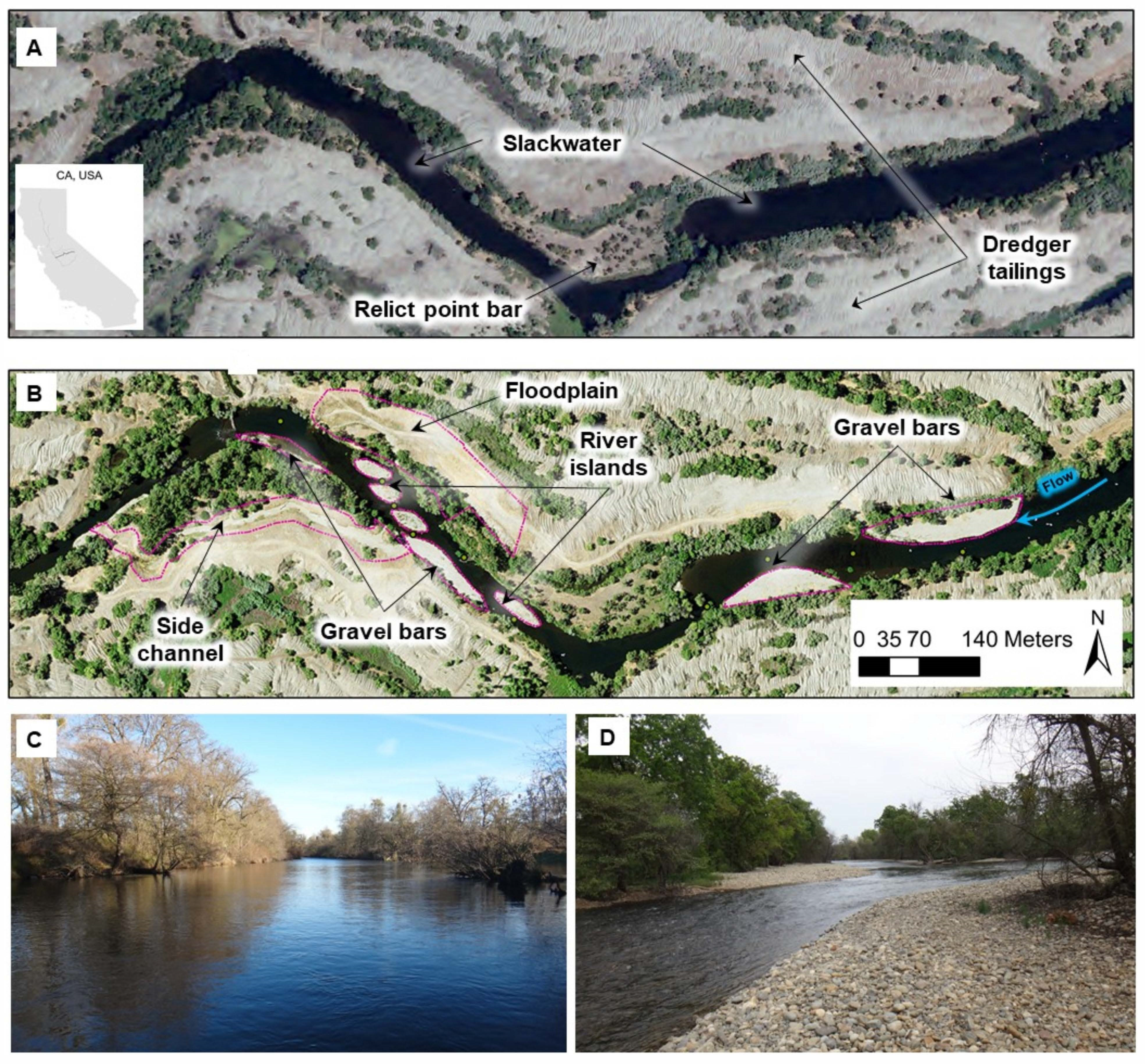
2.3.3. Floodplain and Side Channels

Many floodplains in river corridors subject to rescaling are so altered that empirical geomorphologic predictive relationships based on unregulated, natural conditions likely have little to no relevance. Because regulated flows are usually lower than historic conditions, and channels are usually incised because of the reduced sediment supply, off channel restoration usually involves lowering adjacent gravel bars, terraces and historical floodplains to allow inundation at newly prescribed flows [39]. In some cases, the lowering of relic floodplains is often pursued in tandem with main channel gravel augmentation to rebuild the channel bed [39]. Existing flood control and adjacent infrastructure often limit the extent of restored floodplains, necessitating a quantitative basis for optimizing physical habitat within these constraining features.

Key attributes include at a minimum the elevation, length, and width (areal size) of the floodplain and any side channels. Far fewer empirical relationships exist for floodplain and side channel size based on channel width than river planform and profiles. Hydrogeomorphic predictors of floodplain elevation or height is not explicitly addressed in the literature. However, it can be initially approximated by setting floodplain elevation equal to the channel elevation plus the bankfull depth at riffles. Assuming floodplain width can be approximated by meander belt width there are also hydrogeomorphic equations to predict floodplain width. Using data from 153 locations, Williams [67] derived the following expression to predict floodplain width ($W_{FP})$ using from $W_{BF}$:

$$W_{bf}=4.3W_{bf}{}^{1.12}$$

(9)

Note that this relationship assumes that the floodplain only needs to be as wide as the meander belt width, and ignores other potential factors related to floodplain size such as flood control and Pacific salmon habitat needs. Further, like other empirical relationships it assumes that natural processes occur in the absence of a human impact.

Side channels are also often created and/or enhanced for juvenile rearing habitat, sometimes nested within the bankfull channel, or created as independent features [28]. There are few analytical and empirical relationships for predicting relative size of side channels using hydrogeomorphic scaling. Stability diagrams based on one-dimensional bifurcation models can help assess stability of potential side channel configurations over time [132]. In practice, many of these features are designed using simple initial conditions and refined in form–process–habitat modeling and iteration.

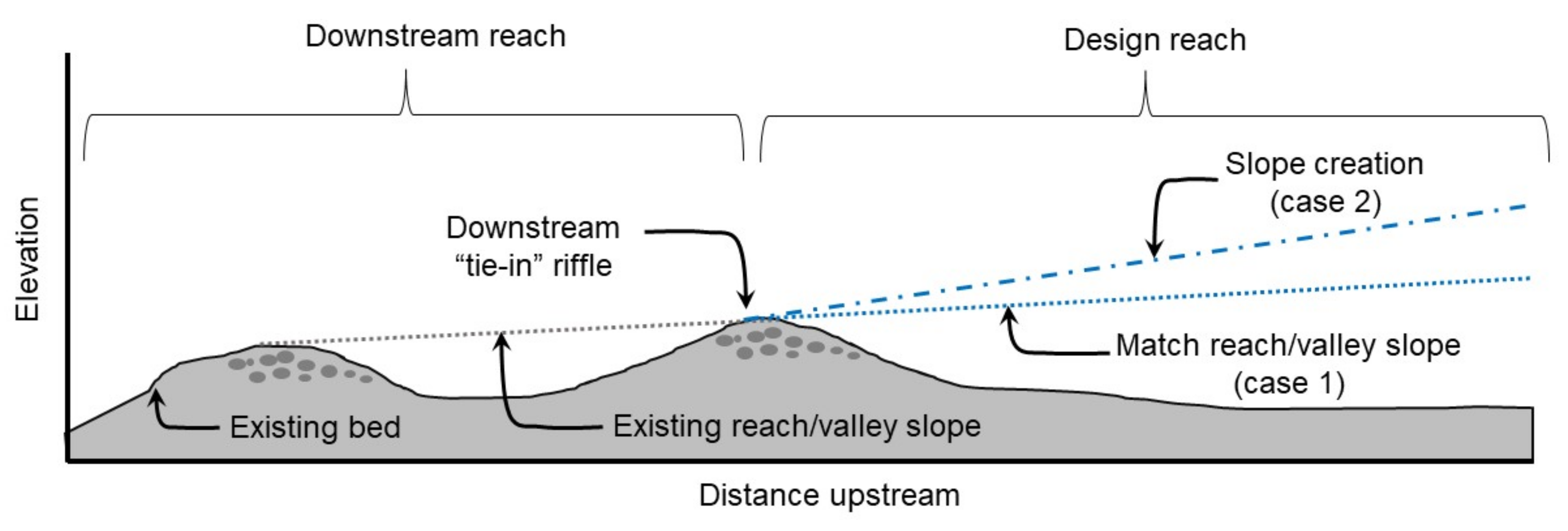
2.4. Pool–Riffle Variation

While modal conditions of the rescaled bankfull channel geometry are important to determine planform typology and scaling, they do not explicitly inform riffle–pool geometry. Undulating bed relief, in the form of riffle–pool sequences, is thought to be a fundamental attribute of cobble–gravel alluvial rivers providing hydraulic, sedimentary and water quality characteristics needed for Chinook salmon spawning [17,133]. Variation in bed elevation and inundation width is a fundamental attribute of alluvial river morphology [17,134,135,136,137], with linkages between channel morphology and fish habitat utilization [17,138]. Key geometric aspects include determining the spacing, length, width, and depth of riffle–pool sequences.

Similar to meander geometry, gravel and cobble alluvial bedforms are thought to scale to the mean bankfull channel width [139], although others suggest flow and flow depth can also be a scaling variable [140]. Gravel and cobble alluvial bar–pool bedform scaling can be represented as:

$${\lambda }_{bed}=a_{bed}{W}_{bf}$$

(10)

where ${\lambda }_{bed}$ is the wavelength of bed oscillations and $a_{bed}$ is an empirical coefficient that can range from 1.5 to 28 [141], with a modal range of 5–7 [139,142]. The modal range of $a_{bed}$ has been explained by theory [119,121,143], field [139,142] and flume [144] studies. Since the bed profile is coupled with the alignment of the channel in meandering rivers, it follows that ${\lambda }_{bed}$ should be roughly half of ${\lambda }_m$. The parameter $a_{bed}$ can be thought of representing how equilibrated the river system is relative to its flow and sediment regime. For example, Carling and Orr [142] suggest that $a_{bed}$ = 3 is representative of nascent bedforms that have yet to equilibrate, while $a_{bed}$ > 7 can occur due to channelization or reductions in sediment supply [145]. Wilkinson et al. [120] propose that freely migrating lowland alluvial rivers may tend towards a more regular value of $a_{bed}$, while mountain rivers with forcing elements may lead to structural controls on riffle–pool spacing and greater variability. This is supported by field measurements of pool spacing in forest channels [146], where higher densities of forcing elements such as woody material can yield $a_{bed}$ < 3. The implication is that if one is completely resetting the river corridor or designing a freely alluvial river then modal spacing values are useful. However, in confined or constrained settings local variation in the available river corridor width from bedrock, vegetation or even hardened infrastructure can also serve to locate riffles and pools beyond reach-averaged scaling values.

An additional consideration for bedform spacing is exclusion length theory, which suggests that at a constriction or pool forming element there is a relatively constrained downstream distance where a non-pool bedform would likely not occur, generally on the order of 1–3 $W_{bf}$ based on statistical modeling and field observations [147,148,149,150,151]. Thompson (2001) suggests that using a fixed spacing can prohibit adjustment from environmental change [23]. Rather, it is recommended that there is a minimum distance between bedforms so they can absorb environmental change by having the space or capacity for adjustment.

The length of riffle–pool units can be inferred from meander geometry, bedform scaling relationships or from empirical relationships. Based on theory, Yalin [143] proposed that for equilibrium dunes, the length $\left(L_d\right)$ should scale with depth $\left(H\right)$ as $L_d=\alpha 2\pi H$, where $\alpha$ ranges from 1 to 6 according to limited field verification [142]. If a single bed oscillation consists of only a riffle and a pool with no transitional morphologic units then riffle $\left(L_r\right)$ and pool lengths $\left(L_p\right)$ can be assumed to be half the spacing, so that $L_r=L_p=\frac{1}{2}{\lambda }_{bed}$. Empirical studies have shown that there are sometimes transitional units such as chutes, runs, and glides [152,153] that could occupy areas between the riffle and pool. Field studies have shown that riffle length can range from 1.3 to 4.5 W and most show $L_r$ equal to or greater than $L_p$ [149,154]. A driver in this variance is gradient, as on average both riffles and pools become longer and asymmetric as gradient decreases [154].

The relative width and depth of riffles and pools can be determined from empirical and physics-based relationships. Empirical relationships between average channel width and the width for riffles and pools (e.g., [85]) likely suffer the same constraints that limit purely empirical predictors of channel geometry. The Caamaño relationship can be used to relate bankfull riffle and pool widths and depths for conditions where riffle–pool maintenance would be likely based on the concept of a velocity reversal [155]. The relationship takes the form:

$$\frac{w_r}{w_p}=1+\frac{h_{pz}}{h_r}$$

(11)

where $w_r$ is the width of the riffle, $w_p$ is the pool width, $h_r$ is the riffle depth, and $h_{pz}$ is the residual pool depth equal to $h_r-h_p$, where $h_p$ is the pool depth at the flow of interest (Figure 5A,B). This equation has been used to recreate the topography of alluvial riffle–pool topography that would experience flow convergence routing, a key hydrogeomorphic mechanism for maintaining riffle–pool relief [41]. Equation (11) could be used in a variety of ways depending on what are considered independent and dependent variables. For example, by assuming $h_r$ is equal to $H_{bf}$ (Equation (2)) and using with a relationship or value for permissible velocity for stable $D_{50}$, $w_r$ could be determined from the continuity equation. Empirical relationships for pool depth or width could be used to solve for the other unknowns, such as relationships for meander bend scour or bed scour at constrictions that can estimate $h_p$ based on $w_p$ [120,156].

2.5. Which Hydrogeomorphic Scaling Relationships, or Does It Even Matter?

Different hydrogeomorphic relationships will yield different results, and there are no studies that have explicitly evaluated whether one approach or set of equations is better for designing gravel–cobble bed rivers for salmonid habitat than another. However, some studies do evaluate their utility in predicting current channel form [95,96]. Since reach averaged bankfull geometry estimates are used to develop initial geometries that are ultimately iterated for form–process–habitat linkages this initial uncertainty may have little consequences. For a reach of the Merced River below Crocker-Huffman Dam in California, four predictive equations indicate that the coefficient of variations in depth and width predictions are relatively small (

Table 1. Predicted bankfull width, depth and slope for the Merced River below Crocker-Huffman Dam in California, USA using Equations (2) and (3) in this paper, the University of British Columbia regime model (UBCRM, [65]) and relationships by Parker et al. [103], Hey and Thorne [85]. Input scaling variables are $Q_{bf}=$ 59.5 m³/s, $D_{50}=$ 0.032 m, $S=$ 0.002.

Source	Width (m)	Depth (m)	W/D	Assumptions
UBCRM (Eaton and Millar 2017)	28.7	1.40	20.4	μ’ = 0.98/ Type I vegetation
Parker et al., 2007	29.5	1.26	23.5	r = 1.5
Equations (2) and (3)	31.7	1.26	25.2	r = 1.5
Hey and Thorne, 1983	32.6	1.43	22.8	Type I vegetation
Average	30.6	1.34	23.0
Standard deviation	1.59	0.08	1.73
Coefficient of variation	0.05	0.06	0.08

). The standard deviation of predicted depths in Table 1 are within average construction tolerances for working in flowing gravel bed streams (e.g., 0.15 m [157]). Further, while channel width and depth predictions drive the scaling of planform geometry they are ultimately iterated upon after via form–process–habitat iteration. This reinforces that these equations are essentially guides to river design and are not meant to be strictly reinforced. Moreover, when building these types of projects, it is not uncommon to slightly adjust in the field to achieve specific hydraulic design criteria for depth, velocity, and water surface gradient.

The uncertainty in the bankfull geometry can be handled through Monte Carlo simulations [65,158]. Given that gradient is usually held constant and median substrate is specified for salmonid spawning, the two primary sources of variance are the channel forming discharge and bank resistance. Bank resistance could be calibrated by analyzing observed or adjacent reaches [65]. A representative discharge is one of the largest sources of uncertainty [158]. The University of British Columbia Regime Model (UBCRM) regime model for channel geometry has built in capabilities to consider the role of uncertainty in scaling variables on predictions of $H_{bf}$ and $W_{bf}$ [65]. For example, for the same reach in Table 1 factoring in uncertainty for 20% of the values of $Q_{bf}$ and bank strength yields a wider range of possible $W_{bf}$ compared to $H_{bf}$ (Figure 6). How this uncertainty propagates to other aspects such as planform typology and scaling can be explored using similar methods.

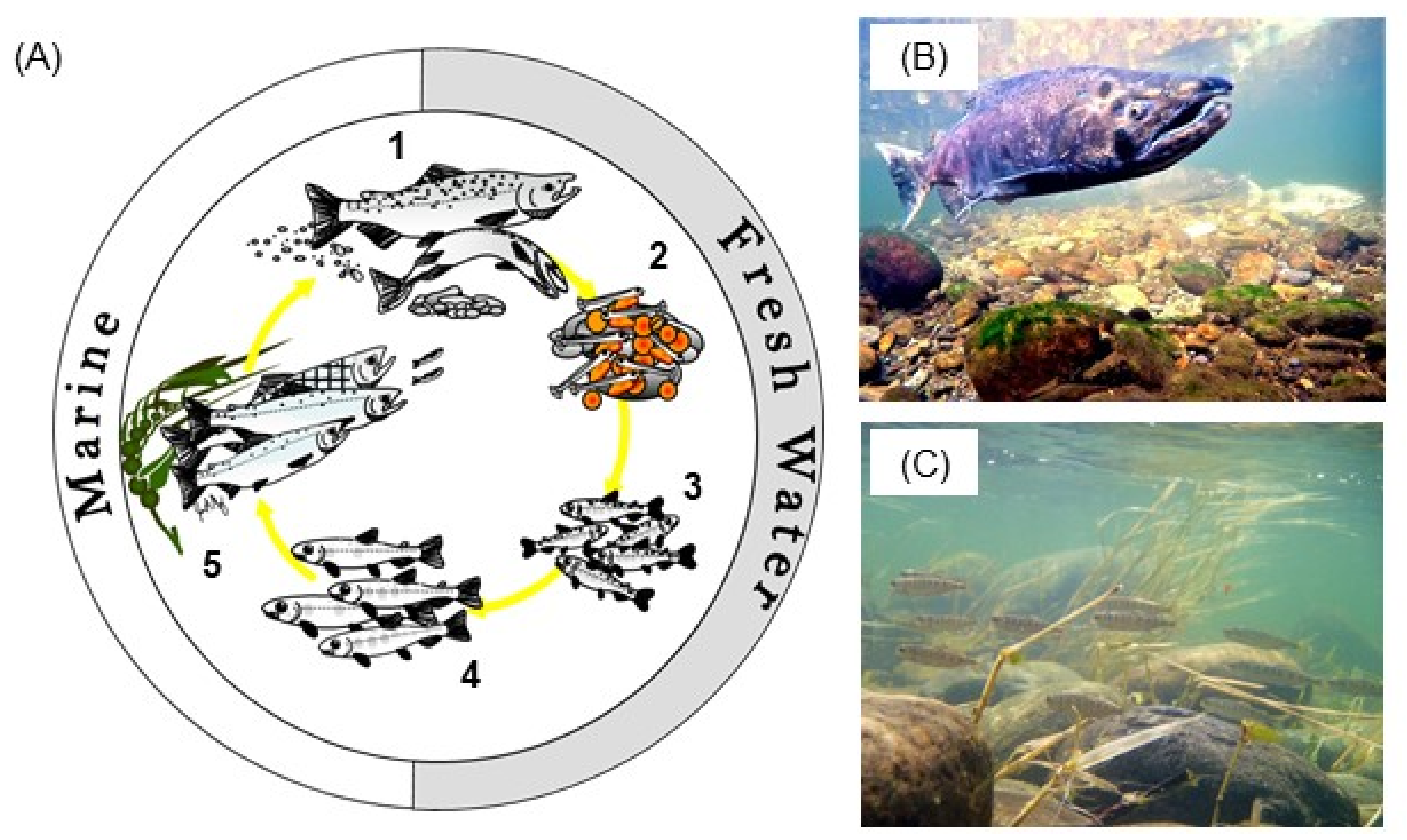
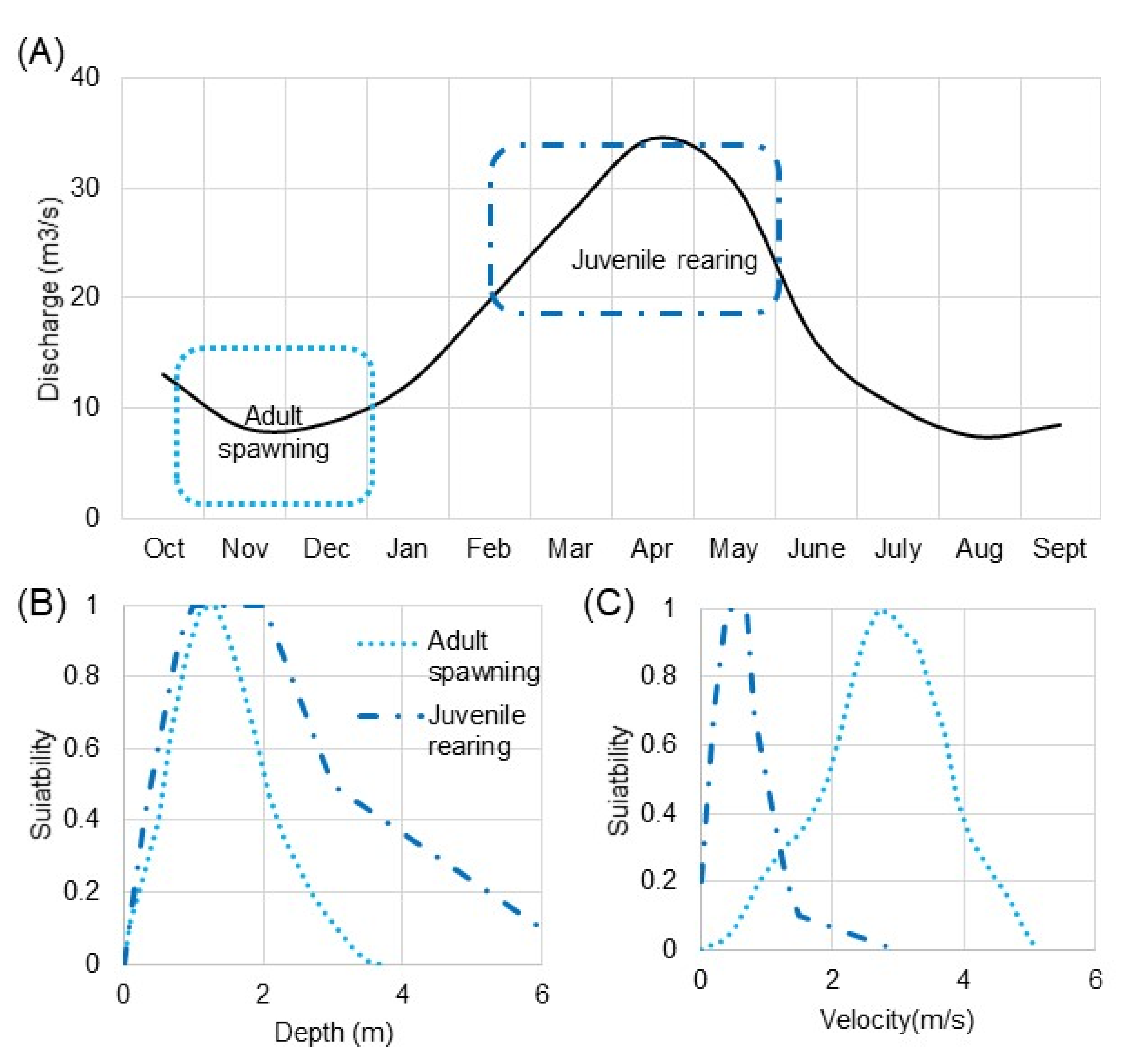
3. Ecohydraulic Scaling for Salmon Habitat

Ecohydraulic scaling uses hydraulic habitat suitability criteria and basic open channel flow relationships to determine the size of channel and floodplain morphologic features for optimum or modal conditions for specific species and life stages (Figure 3). Habitat preferences can be determined from hydraulic habitat suitability curves (Figure 7), which can specify ranges of preferred conditions for utilization by aquatic organisms, most commonly for depth and velocity, although water temperature and sediment size may be included, too [159]. By selecting discrete modal values, or ranges of depth and velocity for relevant ecohydrology, channel geometry can be optimized for simple cases that are adequate for initial design using basic open channel flow equations. The use of 1D hydraulics approaches to evaluate salmon habitat restoration designs are not without criticism [160], but they provide quick estimates of initial dimensions that can be evaluated later using numerical models.

Clearly defining the species and life-stage helps constrain the range of hydrologic and hydraulic requirements needed. There are a variety of salmonid species and depending on their life history they can use different types of river channels and habitat features during different times of the year [161]. Even for a single species, there is considerable variation in the needs of different life stages, as juvenile rearing salmon use different riverine habitat features compared to adult spawners [73,162] (Figure 1). Most salmonid habitat restoration projects that rescale river corridors consider all life stages, although ecohydraulic design is most tractable for juvenile rearing and adult spawning habitat.

Ecohydrology is developed by relating the temporal range of the life stage(s) to relevant hydrology for that period (Figure 7). Average flows are shown in this case, but other statistical measures could be used as well as consideration of flow duration. For spawning Pacific salmon common considerations are to use the mean monthly flow during the spawning period, as well as minimum flows for upstream passage as well as flow fluctuations that could lead to redd dewatering. For rearing salmon habitat, ecohydrology can be based on broad considerations such as frequently activated floodplains [163], or by determining seasonal flow scenarios that have different combinations of frequency and duration [39]. For example, the Hydrologic Engineering Centers Ecosystem Functions Model (HEC-EFM) is capable of exploring a variety of statistical scenarios to develop ecohydrology [164].

With representative ecohydrology, the continuity equation along with average depth and velocity requirements for a specific species and life stage (Figure 6) determine a reach-averaged width for a feature such as a riffle, side channel or floodplain at the flow of interest. Assuming steady, uniform flow, and a rectangular channel for simplicity, the continuity equation is:

$$Q=WHV$$

(12)

where $Q$ is water discharge, $W, H$ and $V$ are the average width, depth and velocity [165]. Since ecohydrology specifies the flow, and ecohydraulics can inform the average velocity and depth, the width for a given mesohabitat $\left(W_{mu}\right)$ can easily be solved:

$$W_{mu}=\frac{Q_{lifestage}}{V_{suitable} H_{suitable}}$$

(13)

While simple, this helps constrain the approximate geometry of features and the space needed for them in planform beyond hydrogeomorphic considerations. For example, spawning riffle flow widths can be estimated by using modal values of suitable depth and velocity along with a representative spawning flow. For spawning riffles a subtle layer of sophistication can be added by using a flow resistance equation to predict the average velocity. Depending on the riffle crest configuration Weir equations can also be used [166].

This same approach can be used for off-channel features such as floodplains and side-channels for juvenile rearing, if assumptions can be made about how flows are distributed over these features. The amount of flow available for off-channel features ($Q_{off-channel})$ can be assumed to be equal to the difference between the juvenile rearing design flow and the bankfull discharge ($Q_{rearing }-Q_{bankfull }$). Assumed amounts of $Q_{off-channel}$ can then be used with modal estimates of suitable depth and velocity for rearing salmon in Equation (13) to develop the width of off-channel features. While real-world off-channel habitats such as side channels and floodplains are often complex and may not behave according to the uniform, steady flow assumptions within all areas of the floodplain, this simple approach can provide a generalized width that can help inform the overall rescaled design geometry.

Figure 7. Examples of ecohydrology and ecohydraulics. Ecohydrology (A) entails relating species and/or life stages with seasonal hydrology. In this case monthly average flow is shown for the Merced River, CA USA near the town of Snelling from 1994 to 2017 along with primary adult spawning and juvenile rearing periods for fall-run Chinook Salmon. Note that other life stages are important to consider (see Figure 1) but are omitted for clarity. Ecohydraulics utilizes habitat suitability curves to determine the range and optimal depths (B) and velocities (C) needed for a given life stage and are applied to the flows relevant to that life stage. The curves shown here are for fall-run Chinook Salmon spawning [167] and rearing [168].

Figure 7. Examples of ecohydrology and ecohydraulics. Ecohydrology (A) entails relating species and/or life stages with seasonal hydrology. In this case monthly average flow is shown for the Merced River, CA USA near the town of Snelling from 1994 to 2017 along with primary adult spawning and juvenile rearing periods for fall-run Chinook Salmon. Note that other life stages are important to consider (see Figure 1) but are omitted for clarity. Ecohydraulics utilizes habitat suitability curves to determine the range and optimal depths (B) and velocities (C) needed for a given life stage and are applied to the flows relevant to that life stage. The curves shown here are for fall-run Chinook Salmon spawning [167] and rearing [168].

Other applications of ecohydraulics include using minimum depths and maximum velocities for upstream migration. Depending on fish body size there are different criteria for minimum depths over riffles at minimum or low flows. Maximum velocities for swimming fish are based on the concept of swimming modes, with different durations that a fish can swim in those modes. Swimming modes for fish can be classified as cruising, sustained or darting [169]. Metabolic requirements for the fish increase from cruising to darting swimming modes, and as a result fish usually swim for shorter durations, although water temperature and dissolved oxygen play an important role. For example, the maximum length of high velocity areas of habitat features can be bounded by fish swimming abilities. The maximum distance a salmon can travel under darting $(L_{max})$ can be determined by relating maximum darting speeds ($V_{darting})$ to the time to exhaustion $(T_{exhaustion})$ as:

$$L_{max}=V_{darting}{T}_{exhaustion}$$

(14)

In this case, $L_{max}$ represents the distance where a fish would be exhausted and lose the ability to swim upstream.

Habitat capacity concepts can also inform the relative size of habitat features. If population targets specific to restoration actions are available, the size of features could also be estimated by assuming fish densities (number of fish per area) at different life stages. The basic relationship is:

$$L_{mu}=\left(\frac{\# fish}{fish density}\right)/W_{mu}$$

(15)

For example, spawning riffle width can be determined from Equation (13), but then the length can be determined based on how many spawners are desired, or possible, per riffle based on estimates of redd areas. Salmon redd size varies with species, fish size, substrate, and other factors, but for Chinook salmon they generally range from 9 to 10 m² [170,171]. Similarly, stream rearing juvenile salmonids can express territorial behaviors over a certain distance depending on their body size, yielding relationships between fish size and area needed [172]. Therefore, if an estimate of the number of juvenile salmon desired for specific fish sizes is available, then Equation (15) can be used to estimate the length of the unit.

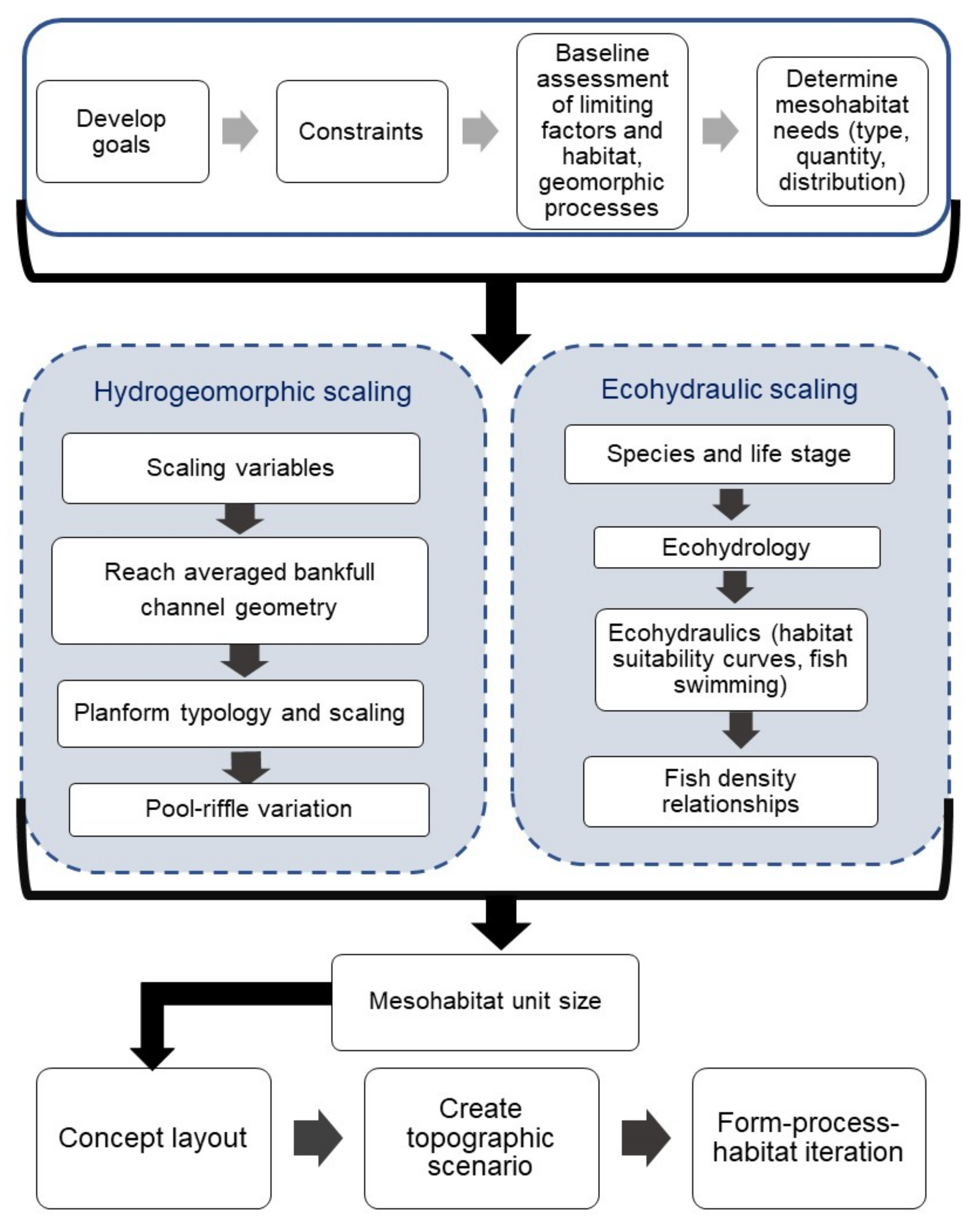
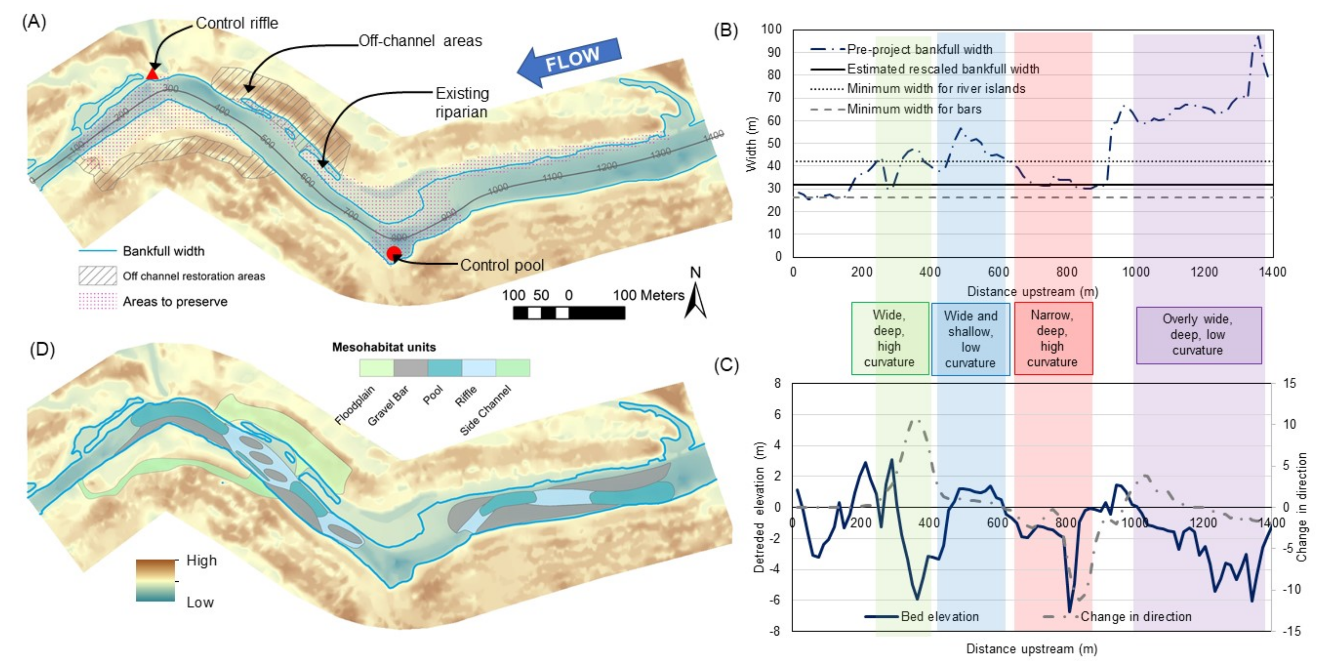
4. Creating Conceptual Mesohabitat Unit Designs

The above sections provide a way to determine the size and shape of habitat restoration features based on hydrogeomorphic scaling and ecohydraulics, but how are these dimensions used to develop river restoration design scenarios? While one could develop topographic scenarios immediately following methods in [48,173], in practice it is common to first develop and lay out polygons for design alternatives that represent a combination of geomorphic and mesohabitat unit characteristics. A foundation for developing the application of the ecohydraulic-based mesohabitat unit approach for stream restoration design is described by [58]. Open-source platforms such as QGis and GoogleEarth can easily be utilized to create conceptual mesohabitat design polygons. The hydrogeomorphic and ecohydraulic scaling relationships presented here can help define the areal extent of these features, allowing an evaluation of how the rescaled river morphology will be nested in the existing river corridor. The use of mesohabitat units allows a simple quantification of habitat areas, which along with life stage specific habitat densities can allow an estimation of potential habitat improvement. Similarly, utilizing realistic river channel scenarios allows at least a conceptual evaluation of form-process linkages. Together, they allow alternative restoration strategies to be evaluated prior to the development of more complex topographic and numerical models [174,175].

An often-overlooked aspect of river restoration design is how to specify the location of mesohabitat units. When a river is completely realigned free of external constraints the location of mesohabitat units can follow basic archetypal relationships of alternate bar geometry [35,36] (Figure 5). However, more complex or longer cases are common where rescaled mesohabitat units are nested within the current river planform [39]. In these cases, an important first step is to identify and locate existing constraints on controls that features would need to be worked around, such as existing biological resources (Figure 8A). Next, the current bankfull and river corridor width is compared to the widths needed for different planforms or bar modes to see where different river bar types are possible (Figure 8B). Flow alignments for different flows are developed based on the concept of topographic steering [176] and existing curvature in the river channel. The inclusion of topographic steering is relatively simple as it requires the designer to envision the desired paths of water flow for different stages. Once an alignment is developed, riffle, pool and bar units can be located based on archetypical relationships of alluvial rivers, easily leveraged using the concept of geomorphic covariance structures (GCS; Figure 8C). Note that other mesohabitat units exist and could be used. A GCS is a bivariate spatial relationship among variables along a pathway in a river corridor. Examples include the covarying relationships between bed elevation, channel width and curvature for riffles [134,177,178,179], pools [148,149,151], lateral gravel bars [134,180,181,182] and river islands [109,183] (

Table 2. Archetypal geomorphic covariance structure (GCS) relationships for riffle, pool, gravel bar and river island mesohabitat units.

Mesohabitat Unit	Example(s)	GCS Relationship	Citations
Riffle	Riffles located at point bar crossover	Low curvature, wider than average, higher than average bed elevation	[128,171,172,173]
Pool	Pools located adjacent to river bends or adjacent to gravel bars and forcing elements	High curvature, narrower than average, lower than average bed elevation	[146,147,149,174]
Lateral gravel bar	Gravel bars located on inward side of bend or downstream of an obstruction	High curvature, wider than average at bankfull and greater flow	[128,144,175,176]
River island	Islands located in channel expansions and/or after channel bends	Wider than average, low curvature at bankfull or greater flow	[94,177]

). Once the above information is assessed, mesohabitat units are sited starting with the upstream or downstream control units using predicted wavelength and exclusion lengths (Figure 8D). An important consideration is that calculated wavelengths should be taken as flexible estimates, as modal values from the literature represent data sources with relatively high variance. Less design guidance is available for off-channel features as these tend to be driven more by the availability of land for habitat rehabilitation or flood control. Although for side channels the authors of [132] suggest that they should be located preferably downstream of an outer bend or at the inside of a mild bend to increase resilience. While rare, in some cases agricultural uses are compatible with the inundation regime needed to support juvenile salmon growth [74].

5. Discussion

Restoring rivers through topographic manipulation is founded on the notion that created forms will yield specific processes and habitat. This is confounded by the nonlinear nature of fluvial systems and equifinality, or put more simply, forms can be created and maintained by different processes. Nonetheless, leveraging what we currently know about rivers can aid us in understanding the general size of geomorphic and mesohabitat units relevant to Pacific salmon habitat restoration. Obviously, the equations presented herein are simplifications that do not convey the diversity of riverine forms. Human creativity can add diversity to river designs, but it runs the risk of being unbounded and/or purely artistic. Ecohydraulics is useful in this context because it essentially provides an additional set of bounds on the size and shape of features, akin to an additional extremal constraint to predicting alluvial channel geometry [89]. The literature has shown that ecohydraulic design can yield immediate usage of habitat validating the use of physical habitat models in iterative design [25,26,36,39,45,47,184,185]. Lastly, the use of numerical models in modern river design in form–process–habitat iterations provides a tested a way of evaluating designs so that they can be optimized beyond initial configurations [26,44,186].

An important component of resizing a river corridor for fish habitat is how it evolves from the point of construction into the future. These concepts could be applied to fully mobile or engineered stable designs but building completely static river corridors that experience minimal channel change runs counter to restoring river corridors for salmonids. Rather, these concepts are best applied when combining form and process-based restoration [41,60], where initial forms are sculpted but then expected to naturally evolve over time via hydrogeomorphic and biomorphic processes. While form–process iteration can optimize river corridor geometry, these linkages can be lost when there is significant change that alters the morphology. How rivers evolve in these settings is driven by not only fluvial processes, but ecosystem engineers and the human management of flow and sediment.

Plants are well known ecosystem engineers that can control channel geometry, planform and overall morphology [22,101,113,187]. In many regulated rivers, especially in Mediterranean climates, vegetation encroachment can simplify channel geometry and degrade salmonid habitat [188,189,190]. When developing a rescaled river corridor there should be some foresight into these processes, although the practical application of these concepts is tenuous due to the dominant effects of flow regime on riparian plant evolution. That is, even if river corridors are rescaled, over time the flow regime will likely contribute significantly to riparian plant recruitment and associated ecogeomorphic feedbacks that can degrade channel form over time. This highlights the role of coupling flow and form-based restoration strategies for salmonids [8].

Regulated rivers where topographic rescaling occurs often have little to no natural coarse sediment supply. While flow is commonly regulated for aquatic organisms such as salmonids, sediment is often not considered in this context [191], although cases do exist [29]. Ultimately, sediment transport is essential to restoring salmonid habitat because spawning salmon must biophysically disturb the riverbed at least on par with the average depth of redd construction, approximately 0.5 m [192], to construct a redd. Since riffles usually serve as important hydraulic controls [193] this means that the restoration of alluvial river morphology for salmon habitat requires both dynamism and stability over different time scales. The riverbed needs be dynamic enough during moderate flow and biophysical stresses to allow redd construction, but also stable enough over larger flows so that population gains can be achieved through habitat restoration over some period. The only way for these two somewhat contradictory goals to be achieved is through synchronizing flow, form and sediment supply. Synchronous flow and form are recognized as important components of river restoration [8,18,19,194], but along with this a sediment budget is needed that is also synchronous with the flow regime, especially for reaches immediately below dams [191,195]. Remote sensing, field monitoring and differencing of topographic maps to yield sediment budgets provide a tested and easy way to track river and habitat evolution over time [36,37,47]. Similar to other forms of river restoration, gains from rescaling alluvial river morphology may ultimately diminish if not maintained [196].

6. Conclusions

This paper presented a review of how hydrogeomorphic and ecohydraulic scaling can be used to determine initial of size of rescaled channel and floodplain mesohabitat units in regulated gravel–cobble bed rivers for Pacific salmon habitat. Hydrogeomorphology and ecohydraulics are necessary and complimentary components of Pacific salmon habitat restoration, representing the physical and biological sciences, respectively. When used together they help objectively inform the geomorphic potential and resulting habitat capacity associated with river restoration designs aimed at improving physical habitat for Pacific salmon. Presenting these two ideologies on parallel footing helps emphasize the need to jointly consider physical forms and biological processes in developing designs for Pacific salmon habitat restoration in regulated rivers. Further, the transparent presentation of these relationships allows an open critique, that may, over time, advance the science of river restoration design. More comparative studies are needed to better understand differences in these approaches, or if they even matter at all over time, highlighting the need for long term monitoring and synthesis. Lastly, it is important to be mindful that even if river corridors can be rescaled to new flow regimes, management, and maintenance of created habitat will be needed in these Anthropocene rivers.

References

1. Trush, W.J.; McBain, S.M.; Leopold, L.B. Attributes of an alluvial river and their relation to water policy and management. Proc. Natl. Acad. Sci. USA 2000, 97, 11858–11863. [Google Scholar] [CrossRef] [PubMed] [Green Version]
2. Kondolf, G.M.; Podolak, K.; Grantham, T.E. Restoring mediterranean-climate rivers. Hydrobiologia 2013, 719, 527–545. [Google Scholar] [CrossRef]
3. Wheaton, J.M.; Pasternack, G.B.; Merz, J.E. Spawning habitat rehabilitation-I. Conceptual approach and methods. Int. J. River Basin Manag. 2004, 2, 3–20. [Google Scholar] [CrossRef]
4. Wohl, E.; Lane, S.N.; Wilcox, A.C. The science and practice of river restoration. Water Resour. Res. 2015, 51, 5974–5997. [Google Scholar] [CrossRef] [Green Version]
5. Johnson, M.F.; Thorne, C.R.; Castro, J.M.; Kondolf, G.M.; Mazzacano, C.S.; Rood, S.B.; Westbrook, C. Biomic river restoration: A new focus for river management. River Res. Appl. 2020, 36, 3–12. [Google Scholar] [CrossRef] [Green Version]
6. Pasternack, G.B. River Restoration: Disappointing, Nascent, Yet Desperately Needed. In Reference Module in Earth Systems and Environmental Sciences; Elsevier: Amsterdam, The Netherlands, 2020. [Google Scholar]
7. Bernhardt, E.S.; Palmer, M.A.; Allan, J.D.; Alexander, G.; Barnas, K.; Brooks, S.; Carr, J.; Clayton, S.; Dahm, C.; Follstad-Shah, J.; et al. Synthesizing U.S. river restoration efforts. Science 2005, 308, 636–637. [Google Scholar] [CrossRef]
8. Whipple, A.A.; Viers, J.H. Coupling landscapes and river flows to restore highly modified rivers. Water Resour. Res. 2019, 55, 4512–4532. [Google Scholar] [CrossRef]
9. Merz, J.E.; Moyle, P.B. Salmon, wildlife, and wine: Marine-derived nutrients in human-dominated ecosystems of central California. Ecol. Appl. 2006, 16, 999–1009. [Google Scholar] [CrossRef] [Green Version]
10. Stanford, J.A.; Ward, J.V.; Liss, W.J.; Frissell, C.A.; Williams, R.N.; Lichatowich, J.A.; Coutant, C.C. A General Protocol for Restoration Of Regulated Rivers. Regul. Rivers Res. Manag. 1996, 12, 391–413. [Google Scholar] [CrossRef]
11. Kondolf, G.M. Hungry water: Effects of dams and gravel mining on river channels. Environ. Manag. 1997, 21, 533–551. [Google Scholar] [CrossRef]
12. Graf, W.L. Downstream hydrologic and geomorphic effects of large dams on American rivers. Geomorphology 2006, 79, 336–360. [Google Scholar] [CrossRef]
13. Grant, G.E. The Geomorphic Response of Gravel-Bed Rivers to Dams: Perspectives and Prospects. In Gravel-Bed Rivers: Processes, Tools, Environments; John Wiley & Sons: Chichester, UK; Hoboken, NJ, USA, 2012; pp. 165–181. ISBN 9780470688908. [Google Scholar]
14. James, L.A.; Singer, M.B.; Ghoshal, S.; Megison, M. Historical channel changes in the lower Yuba and Feather Rivers, California: Long-term effects of contrasting river-management strategies. Spec. Pap. Geol. Soc. Am. 2009, 451, 7. [Google Scholar] [CrossRef] [Green Version]
15. Tockner, K.; Stanford, J.A. Riverine flood plains: Present state and future trends. Environ. Conserv. 2002, 29, 308–330. [Google Scholar] [CrossRef] [Green Version]
16. Yoshiyama, R.M.; Fisher, F.W.; Moyle, P.B. Historical Abundance and Decline of Chinook Salmon in the Central Valley Region of California. N. Am. J. Fish. Manag. 2004, 18, 487–521. [Google Scholar] [CrossRef]
17. Hanrahan, T.P. Bedform morphology of salmon spawning areas in a large gravel-bed river. Geomorphology 2007, 86, 529–536. [Google Scholar] [CrossRef]
18. Jacobson, R.B.; Galat, D.L. Flow and form in rehabilitation of large-river ecosystems: An example from the Lower Missouri River. Geomorphology 2006, 77, 249–269. [Google Scholar] [CrossRef]
19. Brown, R.A.; Pasternack, G.B. Engineered channel controls limiting spawning habitat rehabilitation success on regulated gravel-bed rivers. Geomorphology 2008, 97, 631–654. [Google Scholar] [CrossRef] [Green Version]
20. Tonkin, J.D.; Olden, J.D.; Merritt, D.M.; Reynolds, L.V.; Rogosch, J.S.; Lytle, D.A. Designing flow regimes to support entire river ecosystems. Front. Ecol. Environ. 2021, 19, 326–333. [Google Scholar] [CrossRef]
21. Jager, H.I. Thinking outside the cHannel: Timing pulse flows to benefit salmon via indirect pathways. Ecol. Modell. 2014, 273, 117–127. [Google Scholar] [CrossRef]
22. Hall, A.A.; Rood, S.B.; Higgins, P.S. Resizing a river: A downscaled, seasonal flow regime promotes riparian restoration. Restor. Ecol. 2011, 19, 351–359. [Google Scholar] [CrossRef]
23. Thompson, D.M.; Stull, G.N. The Development and Historic Use of Habitat Structures in Channel Restoration in the United States: The Grand Experiment in Fisheries Management. Géographie Phys. Quat. 2004, 56, 45–60. [Google Scholar] [CrossRef] [Green Version]
24. Ock, G.; Gaeuman, D.; McSloy, J.; Kondolf, G.M. Ecological functions of restored gravel bars, the Trinity River, California. Ecol. Eng. 2015, 83, 49–60. [Google Scholar] [CrossRef]
25. Elkins, E.M.; Pasternack, G.B.; Merz, J.E. Use of slope creation for rehabilitating incised, regulated, gravel bed rivers. Water Resour. Res. 2007, 43, 1–16. [Google Scholar] [CrossRef]
26. Pasternack, G.B.G.B.G.B.; Brown, R.A.R.A.R.A. Ecohydraulic Design of Riffle-Pool Relief and Morphological Unit Geometry in Support of Regulated Gravel-Bed River Rehabilitation. In Ecohydraulics: An Integrated Approach; Wiley: Hoboken, NJ, USA, 2013; pp. 337–355. ISBN 9781118526576. [Google Scholar]
27. Schweizer, S.; Borsuk, M.E.; Reichert, P. Predicting the morphological and hydraulic consequences of river rehabilitation. River Res. Appl. 2007, 23, 303–322. [Google Scholar] [CrossRef]
28. Morley, S.A.; Garcia, P.S.; Bennett, T.R.; Roni, P. Juvenile salmonid (Oncorhynchus spp.) use of constructed and natural side channels in Pacific Northwest rivers. Can. J. Fish. Aquat. Sci. 2005, 62, 2811–2821. [Google Scholar] [CrossRef]
29. Gaeuman, D.; Stewart, R.; Schmandt, B.; Pryor, C. Geomorphic response to gravel augmentation and high-flow dam release in the Trinity River, California. Earth Surf. Process. Landforms 2017, 42, 2523–2540. [Google Scholar] [CrossRef]
30. Merz, J.; Caldwell, L.; Beakes, M.; Hammersmark, C.; Sellheim, K. Balancing competing life-stage requirements in salmon habitat rehabilitation: Between a rock and a hard place. Restor. Ecol. 2019, 27, 661–671. [Google Scholar] [CrossRef]
31. Mörtl, C.; De Cesare, G. Sediment Augmentation for River Rehabilitation and Management—A Review. Land 2021, 10, 1309. [Google Scholar] [CrossRef]
32. James, L.A. Designing forward with an eye to the past: Morphogenesis of the lower Yuba River. Geomorphology 2015, 251, 31–49. [Google Scholar] [CrossRef] [Green Version]
33. Marchetti, M.P.; Moyle, P.B. Effects of flow regime on fish assemblages in a regulated California stream. Ecol. Appl. 2001, 11, 530–539. [Google Scholar] [CrossRef]
34. Kiernan, J.D.; Moyle, P.B.; Crain, P.K. Restoring native fish assemblages to a regulated California stream using the natural flow regime concept. Ecol. Appl. 2012, 22, 1475–1482. [Google Scholar] [CrossRef] [PubMed]
35. Downs, P.W.; Singer, M.S.; Orr, B.K.; Diggory, Z.E.; Church, T.C. Restoring ecological integrity in highly regulated rivers: The role of baseline data and analytical references. Environ. Manag. 2011, 48, 847–864. [Google Scholar] [CrossRef] [PubMed]
36. Harrison, L.R.; Legleiter, C.J.; Wydzga, M.A.; Dunne, T. Channel dynamics and habitat development in a meandering, gravel bed river. Water Resour. Res. 2011, 47, W04513. [Google Scholar] [CrossRef] [Green Version]
37. Roni, P.; Hall, J.E.; Drenner, S.M.; Arterburn, D. Monitoring the effectiveness of floodplain habitat restoration: A review of methods and recommendations for future monitoring. WIREs Water 2019, 6, e1355. [Google Scholar] [CrossRef]
38. Harrison, L.R.; Bray, E.; Overstreet, B.; Legleiter, C.J.; Brown, R.A.; Merz, J.E.; Bond, R.M.; Nicol, C.L.; Dunne, T. Physical Controls on Salmon Redd Site Selection in Restored Reaches of a Regulated, Gravel-Bed River. Water Resour. Res. 2019, 55, 8942–8966. [Google Scholar] [CrossRef]
39. Cramer Fish Sciences. Merced River Ranch and Henderson Park Restoration Projects On The Merced River, California. Final Data Report; Cramer Fish Sciences: West Sacramento, CA, USA, 2019. [Google Scholar]
40. Shields, F.D.; Copeland, R.R.; Klingeman, P.C.; Doyle, M.W.; Simon, A. Design for Stream Restoration. J. Hydraul. Eng. 2003, 129, 575–584. [Google Scholar] [CrossRef]
41. Brown, R.A.; Pasternack, G.B.; Lin, T. The Topographic Design of River Channels for Form-Process Linkages. Environ. Manag. 2016, 57, 929–942. [Google Scholar] [CrossRef] [Green Version]
42. Walker, D.R.; Millar, R.G.; Newbury, R.W. Hydraulic design of riffles in gravel/cobble bed Rivers. Int. J. River Basin Manag. 2004, 2, 291–299. [Google Scholar] [CrossRef]
43. Beechie, T.; Pess, G.; Roni, P.; Giannico, G. Setting River Restoration Priorities: A Review of Approaches and a General Protocol for Identifying and Prioritizing Actions. N. Am. J. Fish. Manag. 2008, 28, 891–905. [Google Scholar] [CrossRef]
44. Wheaton, J.M.; Pasternack, G.B.; Merz, J.E. Spawning habitat rehabilitation-II. Using hypothesis development and testing in design, Mokelumne river, California, U.S.A. Int. J. River Basin Manag. 2004, 2, 21–37. [Google Scholar] [CrossRef]
45. Merz, J.E.; Setka, J.D.; Pasternack, G.B.; Wheaton, J.M. Predicting benefits of spawning-habitat rehabilitation to salmonid (Oncorhynchus spp.) fry production in a regulated California river. Can. J. Fish. Aquat. Sci. 2004, 61, 1433–1446. [Google Scholar] [CrossRef] [Green Version]
46. Sellheim, K.L.; Watry, C.B.; Rook, B.; Zeug, S.C.; Hannon, J.; Zimmerman, J.; Dove, K.; Merz, J.E. Juvenile Salmonid Utilization of Floodplain Rearing Habitat After Gravel Augmentation in a Regulated River. River Res. Appl. 2016, 32, 610–621. [Google Scholar] [CrossRef]
47. Wheaton, J.M.; Brasington, J.; Darby, S.E.; Merz, J.; Pasternack, G.B.; Sear, D.; Vericat, D.; Joseph, M.W.; James, B.; Stephen, E.D.; et al. Linking geomorphic changes to salmonid habitat at a scale relevant to fish. River Res. Appl. 2010, 26, 469–486. [Google Scholar] [CrossRef]
48. Brown, R.A.; Pasternack, G.B. How to build a digital river. Earth-Sci. Rev. 2019, 194, 283–305. [Google Scholar] [CrossRef]
49. Wall, C.E.; Bouwes, N.; Wheaton, J.M.; Bennett, S.N.; Saunders, W.C.; McHugh, P.A.; Jordan, C.E. Design and monitoring of woody structures and their benefits to juvenile steelhead (Oncorhynchus mykiss) using a net rate of energy intake model. Can. J. Fish. Aquat. Sci. 2017, 74, 727–738. [Google Scholar] [CrossRef]
50. Lane, B.A.; Pasternack, G.B.; Sandoval Solis, S. Integrated analysis of flow, form, and function for river management and design testing. Ecohydrology 2018, 11, e1969. [Google Scholar] [CrossRef] [Green Version]
51. Wheaton, J.M.; Bouwes, N.; Mchugh, P.; Saunders, C.; Bangen, S.; Bailey, P.; Nahorniak, M.; Wall, E.; Jordan, C. Upscaling site-scale ecohydraulic models to inform salmonid population-level life cycle modeling and restoration actions—Lessons from the Columbia River Basin. Earth Surf. Process. Landforms 2017, 4137, 21–44. [Google Scholar] [CrossRef]
52. Havis, R.N.; Alonso, C.V.; King, J.G. Modeling sediment in gravel-bedded streams using HEC-6. J. Hydraul. Eng. 1996, 122, 559–564. [Google Scholar] [CrossRef]
53. Mosselman, E. Modelling Sediment Transport and Morphodynamics of Gravel-Bed Rivers. In Gravel-Bed Rivers: Processes, Tools, Environments; Wiley: Hoboken, NJ, USA, 2012; pp. 101–115. ISBN 9780470688908. [Google Scholar]
54. Van De Wiel, M.J.; Coulthard, T.J.; Macklin, M.G.; Lewin, J. Embedding reach-scale fluvial dynamics within the CAESAR cellular automaton landscape evolution model. Geomorphology 2007, 90, 283–301. [Google Scholar] [CrossRef]
55. Smith, S.M.; Prestegaard, K.L. Hydraulic performance of a morphology-based stream channel design. Water Resour. Res. 2005, 4, W11413. [Google Scholar] [CrossRef] [Green Version]
56. Harper, D.; Ebrahimnezhad, M.; Climent I Cot, F. Artificial riffles in river rehabilitation: Setting the goals and measuring the successes. Aquat. Conserv. Mar. Freshw. Ecosyst. 1998, 8, 5–16. [Google Scholar] [CrossRef]
57. Taylor Perron, J.; Fagherazzi, S. The legacy of initial conditions in landscape evolution. Earth Surf. Process. Landforms 2012, 37, 52–63. [Google Scholar] [CrossRef]
58. Schwartz, J.S. Use of ecohydraulic-based mesohabitat classification and fish species traits for stream restoration design. Water 2016, 8, 520. [Google Scholar] [CrossRef] [Green Version]
59. Fryirs, K.; Brierley, G. Assemblages of geomorphic units: A building block approach to analysis and interpretation of river character, behaviour, condition and recovery. Earth Surf. Process. Landforms 2021, 47, 92–108. [Google Scholar] [CrossRef]
60. Beechie, T.J.; Sear, D.A.; Olden, J.D.; Pess, G.R.; Buffington, J.M.; Moir, H.; Roni, P.; Pollock, M.M. Process-based Principles for Restoring River Ecosystems. Bioscience 2010, 60, 209–222. [Google Scholar] [CrossRef] [Green Version]
61. Leopold, L.B.; Wolman, M.G. River meanders. Bull. Geol. Soc. Am. 1960, 71, 769–793. [Google Scholar] [CrossRef]
62. Jaeggi, M.N.R. Formation and Effects of Alternate Bars. J. Hydraul. Eng. 1984, 110, 142–156. [Google Scholar] [CrossRef]
63. Crosato, A.; Mosselman, E. Simple physics-based predictor for the number of river bars and the transition between meandering and braiding. Water Resour. Res. 2009, 45, W03424. [Google Scholar] [CrossRef] [Green Version]
64. Crosato, A.; Mosselman, E. An Integrated Review of River Bars for Engineering, Management and Transdisciplinary Research. Water 2020, 12, 596. [Google Scholar] [CrossRef] [Green Version]
65. Eaton, B.; Millar, R. Predicting gravel bed river response to environmental change: The strengths and limitations of a regime-based approach. Earth Surf. Process. Landforms 2017, 42, 994–1008. [Google Scholar] [CrossRef]
66. Schumm, S.A. Meander wavelength of alluvial rivers. Science 1967, 157, 1549–1550. [Google Scholar] [CrossRef] [PubMed]
67. Williams, G.P. River meanders and channel size. J. Hydrol. 1986, 88, 147–164. [Google Scholar] [CrossRef]
68. Maddock, T. Indeterminate Hydraulics of Alluvial Channels. J. Hydraul. Div. 1970, 96, 2309–2323. [Google Scholar] [CrossRef]
69. Doyle, M.W.; Shields, D.; Boyd, K.F.; Skidmore, P.B.; Dominick, D. Channel-Forming Discharge Selection in River Restoration Design. J. Hydraul. Eng. 2007, 133, 831–837. [Google Scholar] [CrossRef]
70. Brown, L.R.; Bauer, M.L. Effects of hydrologic infrastructure on flow regimes of california’s central valley rivers: Implications for fish populationsy. River Res. Appl. 2010, 26, 751–765. [Google Scholar] [CrossRef]
71. Zeug, S.C.; Sellheim, K.; Watry, C.; Wikert, J.D.; Merz, J. Response of juvenile Chinook salmon to managed flow: Lessons learned from a population at the southern extent of their range in North America. Fish. Manag. Ecol. 2014, 21, 155–168. [Google Scholar] [CrossRef]
72. Brown, L.R.; Ford, T. Effects of flow on the fish communities of a regulated California River: Implications for managing native fishes. River Res. Appl. 2002, 18, 331–342. [Google Scholar] [CrossRef]
73. Merz, J.E.; Delaney, D.G.; Setka, J.D.; Workman, M.L. Seasonal Rearing Habitat in a Large Mediterranean-Climate River: Management Implications at the Southern Extent of Pacific Salmon (Oncorhynchus spp.). River Res. Appl. 2016, 32, 1220–1231. [Google Scholar] [CrossRef]
74. Sommer, T.; Harrell, B.; Nobriga, M.; Brown, R.; Moyle, P.; Kimmerer, W.; Schemel, L. California’s Yolo Bypass: Evidence that flood control Can Be compatible with fisheries, wetlands, wildlife, and agriculture. Fisheries 2001, 6, 6–16. [Google Scholar] [CrossRef]
75. Fargione, J.E.; Bassett, S.; Boucher, T.; Bridgham, S.D.; Conant, R.T.; Cook-Patton, S.C.; Ellis, P.W.; Falcucci, A.; Fourqurean, J.W.; Gopalakrishna, T.; et al. Natural climate solutions for the United States. Sci. Adv. 2018, 4, eaat1869. [Google Scholar] [CrossRef] [Green Version]
76. Church, M. Bed Material Transport and The Morphology Of Alluvial River Channels. Annu. Rev. Earth Planet. Sci. 2006, 24, 325–354. [Google Scholar] [CrossRef]
77. Riebe, C.S.; Sklar, L.S.; Overstreet, B.T.; Wooster, J.K. Optimal reproduction in salmon spawning substrates linked to grain size and fish length. Water Resour. Res. 2014, 50, 898–918. [Google Scholar] [CrossRef] [Green Version]
78. Kondolf, G.M.; Wolman, M.G. The sizes of salmonid spawning gravels. Water Resour. Res. 1993, 29, 2275–2285. [Google Scholar] [CrossRef]
79. Fuller, W.B.; Thompson, S.E. The laws of proportioning concrete. Trans. Am. Soc. Civ. Eng 1906, 59, 67–143. [Google Scholar] [CrossRef]
80. Leopold, L.B.; Wolman, M.G. River Channel Patterns: Braided, Meandering, and Straight; Govt. Print. Off.: Washington, DC, USA, 1957; Volume 282-B.U.S. [Google Scholar]
81. Williams, G.P.; Wolman, M.G. Downstream Effects of Dams On Alluvial Rivers; Government Printing Office: Washington, DC, USA, 1984. [Google Scholar]
82. Dade, W.B.; Renshaw, C.E.; Magilligan, F.J. Sediment transport constraints on river response to regulation. Geomorphology 2011, 126, 245–251. [Google Scholar] [CrossRef]
83. Blench, T.; Erb, B. La Théorie Du Régime Appliquée À L’analyse Des Résultats Expérimentaux Concernant Les Transports De Fond. La Houille Blanche 1957, 43, 132–157. [Google Scholar] [CrossRef] [Green Version]
84. Eaton, B.C.; Church, M.; Millar, R.G. Rational regime model of alluvial channel morphology and response. Earth Surf. Process. Landforms 2004, 29, 511–529. [Google Scholar] [CrossRef]
85. Hey, R.D.; Thorne, C.R. Stable Channels with Mobile Gravel Beds. J. Hydraul. Eng. 1986, 112, 671–689. [Google Scholar] [CrossRef]
86. Davidson, S.K.; Hey, R.D. Regime Equations for Natural Meandering. J. Hydraul. Eng. 2011, 137, 894–910. [Google Scholar] [CrossRef]
87. Griffiths, G.A. Stable-channel design in gravel-bed rivers. J. Hydrol. 1981, 52, 291–305. [Google Scholar] [CrossRef]
88. Hoover Mackin, J. Concept of the graded river. Bull. Geol. Soc. Am. 1948, 59, 463–512. [Google Scholar] [CrossRef] [Green Version]
89. Davies, T.R.H.; Sutherland, A.J. Extremal hypotheses for river behavior. Water Resour. Res. 1983, 19, 141–148. [Google Scholar] [CrossRef]
90. Huang, H.Q.; Nanson, G.C. Hydraulic geometry and maximum flow efficiency as products of the principle of least action. Earth Surf. Process. Landforms 2000, 25, 1–16. [Google Scholar] [CrossRef]
91. Huang, H.Q.; Chang, H.H.; Nanson, G.C. Minimum energy as the general form of critical flow and maximum flow efficiency and for explaining variations in river channel pattern. Water Resour. Res. 2004, 40, W04502. [Google Scholar] [CrossRef]
92. Yang, C.T. Formation of Riffles and Pools. Water Resour. Res. 1971, 7, 1567–1574. [Google Scholar] [CrossRef]
93. Copeland, R.R. Application of channel stability methods—Case studies; US Army Corps of Engineers, Waterways Experiment Station: Alexandria, VA, USA, 1994. [Google Scholar]
94. Stroth, T.R.; Bledsoe, B.P.; Nelson, P.A. Full spectrum analytical channel design with the capacity/supply ratio (CSR). Water 2017, 9, 271. [Google Scholar] [CrossRef] [Green Version]
95. Joshi, I.; Dai, W.; Bilal, A.; Upreti, A.R.; He, Z. Evaluation and comparison of extremal hypothesis-based regime methods. Water 2018, 10, 271. [Google Scholar] [CrossRef] [Green Version]
96. Kaless, G.; Mao, L.; Lenzi, M.A. Regime theories in gravel-bed rivers: Models, controlling variables, and applications in disturbed Italian rivers. Hydrol. Process. 2014, 28, 2348–2360. [Google Scholar] [CrossRef] [Green Version]
97. Buffington, J.M.; Montgomery, D.R. A systematic analysis of eight decades of incipient motion studies, with special reference to gravel-bedded rivers. Water Resour. Res. 1997, 33, 1993–2029. [Google Scholar] [CrossRef] [Green Version]
98. Parker, G. Self-formed straight rivers with equilibrium banks and mobile bed. Part 2. The gravel river. J. Fluid Mech. 1978, 89, 127–146. [Google Scholar] [CrossRef]
99. Phillips, C.B.; Jerolmack, D.J. Bankfull Transport Capacity and the Threshold of Motion in Coarse-Grained Rivers. Water Resour. Res. 2019, 55, 11316–11330. [Google Scholar] [CrossRef]
100. Lamb, M.P.; Dietrich, W.E.; Venditti, J.G. Is the critical shields stress for incipient sediment motion dependent on channel-bed slope? J. Geophys. Res. Earth Surf. 2008, 113, F02008. [Google Scholar] [CrossRef] [Green Version]
101. Hickin, E.J. Vegetation and River Channel Dynamics. Can. Geogr./Le Géographe Can. 1984, 28, 111–126. [Google Scholar] [CrossRef]
102. Phillips, R.T.J.; Robert, A. Hydrologic control of waveforms on small meandering rivers. Earth Surf. Process. Landforms 2007, 32, 1533–1546. [Google Scholar] [CrossRef]
103. Parker, G.; Wilcock, P.R.; Paola, C.; Dietrich, W.E.; Pitlick, J. Physical basis for quasi-universal relations describing bankfull hydraulic geometry of single-thread gravel bed rivers. J. Geophys. Res. Earth Surf. 2007, 112, F04005. [Google Scholar] [CrossRef]
104. Millar, R.G. Theoretical regime equations for mobile gravel-bed rivers with stable banks. Geomorphology 2005, 64, 207–220. [Google Scholar] [CrossRef]
105. Copeland, R.R.; Mccomas, D.N.; Thorne, C.R.; Soar, P.J.; Jonas, M.M.; Fripp, J.B. Hydraulic Design of Stream Restoration Projects; Coastal and Hydraulics Laboratory: Washington, DC, USA, 2001. [Google Scholar]
106. Wilcock, P.R.; Crowe, J.C. Surface-based transport model for mixed-size sediment. J. Hydraul. Eng. 2003, 129, 120–128. [Google Scholar] [CrossRef]
107. Eaton, B.C.; Millar, R.G.; Davidson, S. Channel patterns: Braided, anabranching, and single-thread. Geomorphology 2010, 120, 353–364. [Google Scholar] [CrossRef]
108. Kleinhans, M.G. Sorting out river channel patterns. Prog. Phys. Geogr. 2010, 34, 287–326. [Google Scholar] [CrossRef]
109. Wyrick, J.R.; Klingeman, P.C. Proposed fluvial island classification scheme and its use for river restoration. River Res. Appl. 2011, 27, 814–825. [Google Scholar] [CrossRef]
110. Hintz, W.D.; Porreca, A.P.; Garvey, J.E.; Phelps, Q.E.; Tripp, S.J.; Hrabik, R.A.; Herzog, D.P. Abiotic Attributes Surrounding Alluvial Islands Generate Critical Fish Habitat. River Res. Appl. 2015, 31, 1218–1226. [Google Scholar] [CrossRef]
111. Entwistle, N.; Heritage, G.; Milan, D. Ecohydraulic modelling of anabranching rivers. River Res. Appl. 2019, 35, 353–364. [Google Scholar] [CrossRef] [Green Version]
112. Hundey, E.J.; Ashmore, P.E. Length scale of braided river morphology. Water Resour. Res. 2009, 45, W08409–W08447. [Google Scholar] [CrossRef]
113. Kleinhans, M.G.; van den Berg, J.H. River channel and bar patterns explained and predicted by an empirical and a physics-based method. Earth Surf. Process. Landforms 2011, 36, 721–738. [Google Scholar] [CrossRef]
114. Parker, G. On the cause and characteristic scales of meandering and braiding in rivers. J. Fluid Mech. 1976, 76, 457–480. [Google Scholar] [CrossRef]
115. Bledsoe, B.P.; Watson, C.C. Logistic analysis of channel pattern thresholds: Meandering, braiding, and incising. Geomorphology 2001, 38, 281–300. [Google Scholar] [CrossRef]
116. Struiksma, N.; Olesen, K.W.; Flokstra, C.; de Vriend, H.J. Bed deformation in curved alluvial channels. Delft Neth. Delft Hydraul. LAB. Mar. 1985, 23, 57–79. [Google Scholar] [CrossRef]
117. Colombini, M.; Seminara, G.; Tubino, M. Finite-amplitude alternate bars. J. Fluid Mech. 1987, 181, 213–232. [Google Scholar] [CrossRef]
118. Repetto, R.; Tubino, M. Topographic expressions of bars in channels with variable width. Phys. Chem. Earth Part B Hydrol. Ocean. Atmos. 2001, 26, 71–76. [Google Scholar] [CrossRef]
119. Nelson, J.M. The initial instability and finite-amplitude stability of alternate bars in straight channels. Earth Sci. Rev. 1990, 29, 97–115. [Google Scholar] [CrossRef]
120. Wilkinson, S.N.; Rutherfurd, I.D.; Keller, R.J. An experimental test of whether bar instability contributes to the formation, periodicity and maintenance of pool-riffle sequences. Earth Surf. Process. Landforms 2008, 33, 1742–1756. [Google Scholar] [CrossRef]
121. Furbish, D.J.; Thorne, S.D.; Byrd, T.C.; Warburton, J.; Cudney, J.J.; Handel, R.W. Irregular bed forms in steep, rough channels: 2. Field observations. Water Resour. Res. 1998, 34, 3649–3659. [Google Scholar] [CrossRef]
122. Ferguson, R.I. Meander irregularity and wavelength estimation. J. Hydrol. 1975, 26, 315–333. [Google Scholar] [CrossRef]
123. Ackers, P.; Charlton, F.G. Meander geometry arising from varying flows. J. Hydrol. 1970, 11, 230–252. [Google Scholar] [CrossRef]
124. Hey, R.D. Geometry of river meanders. Nature 1976, 262, 482–484. [Google Scholar] [CrossRef]
125. Soar, P.J.; Thorne, C.R. Channel Restoration Design for Meandering Rivers; Coastal and Hydraulics Laboratory: Washington, DC, USA, 2001. [Google Scholar]
126. Ikeda, S. Prediction of alternate bar wavelength and height. J. Hydraul. Eng. 1984, 110, 371–386. [Google Scholar] [CrossRef]
127. Church, M.; Rice, S.P. Form and growth of bars in a wandering gravel-bed river. Earth Surf. Process. Landforms 2009, 34, 1422–1432. [Google Scholar] [CrossRef]
128. Meshkova, L.V.; Carling, P.A. Discrimination of alluvial and mixed bedrock-alluvial multichannel river networks. Earth Surf. Process. Landforms 2013, 38, 1299–1316. [Google Scholar] [CrossRef]
129. Liu, X.; Huang, H.Q.; Nanson, G.C. The morphometric variation of islands in the middle and lower Yangtze River: A variational analytical explanation. Geomorphology 2016, 261, 273–281. [Google Scholar] [CrossRef]
130. Burge, L.M. Stability, morphology and surface grain size patterns of channel bifurcation in gravel-cobble bedded anabranching rivers. Earth Surf. Process. Landforms 2006, 31, 1211–1226. [Google Scholar] [CrossRef]
131. Bolla Pittaluga, M.; Coco, G.; Kleinhans, M.G. A unified framework for stability of channel bifurcations in gravel and sand fluvial systems. Geophys. Res. Lett. 2015, 42, 7521–7536. [Google Scholar] [CrossRef] [Green Version]
132. Van Denderen, R.P.; Schielen, R.M.J.; Blom, A.; Hulscher, S.J.M.H.; Kleinhans, M.G. Morphodynamic assessment of side channel systems using a simple one-dimensional bifurcation model and a comparison with aerial images. Earth Surf. Process. Landforms 2017, 43, 1169–1182. [Google Scholar] [CrossRef] [Green Version]
133. Geist, D.R.; Dauble, D.D. Redd site selection and spawning habitat use by fall chinook salmon: The importance of geomorphic features in large rivers. Environ. Manag. 1998, 22, 655–669. [Google Scholar] [CrossRef]
134. Brown, R.A.R.A.; Pasternack, G.B.G.B. Bed and width oscillations form coherent patterns in a partially confined, regulated gravel-cobble-bedded river adjusting to anthropogenic disturbances. Earth Surf. Dyn. 2017, 5, 1–20. [Google Scholar] [CrossRef] [Green Version]
135. Duffin, J.; Carmichael, R.A.; Yager, E.M.; Benjankar, R.; Tonina, D. Detecting multi-scale riverine topographic variability and its influence on Chinook salmon habitat selection. Earth Surf. Process. Landforms 2021, 46, 1026–1040. [Google Scholar] [CrossRef]
136. Dauble, D.D.; Geist, D.R. Comparison of mainstem spawning habitats for two populations of fall chinook salmon in the Columbia River basin. Regul. Rivers Res. Manag. 2000, 16, 345–361. [Google Scholar] [CrossRef]
137. Shallin Busch, D.; Sheer, M.; Burnett, K.; Mcelhany, P.; Cooney, T. Landscape-level model to predict spawning habitat for lower Columbia river fall Chinook salmon (oncorhynchus tshawytscha). River Res. Appl. 2013, 29, 297–312. [Google Scholar] [CrossRef]
138. Moir, H.J.; Pasternack, G.B. Relationships between mesoscale morphological units, stream hydraulics and Chinook salmon (Oncorhynchus tshawytscha) spawning habitat on the Lower Yuba River, California. Geomorphology 2008, 100, 527–548. [Google Scholar] [CrossRef]
139. Keller, E.A.; Melhorn, W.N. Rhythmic spacing and origin of pools and riffles. Bull. Geol. Soc. Am. 1978, 89, 723–730. [Google Scholar] [CrossRef]
140. Harvey, A.M. Some aspects of the relations between channel characteristics and riffle spacing in meandering. Am. J. Sci. 1975, 275, 470–478. [Google Scholar] [CrossRef]
141. Thompson, D.M. Pool-Riffle. In Treatise on Geomorphology; Academic Press: Waltham, MA, USA, 2013; Volume 9, pp. 364–378. ISBN 9780080885223. [Google Scholar]
142. Carling, P.A.; Orr, H.G. Morphology of Riffle Pool Sequences in the River Severn, England. Earth Surf. Process. Landforms 2000, 4, 369–384. [Google Scholar] [CrossRef]
143. Yalin, M.S. River Mechanics; Peragamon Press: New York, NY, USA, 1971; ISBN 0080401902. [Google Scholar]
144. MacVicar, B.J.; Obach, L.; Best, J.L. Large-Scale Coherent Flow Structures in Alluvial Pools. In Coherent Flow Structures at Earth’s Surface; John Wiley & Sons, Ltd.: New York, NY, USA, 2013; pp. 243–259. ISBN 9781118527221. [Google Scholar]
145. Gregory, K.J.; Gurnell, A.M.; Hill, C.T.; Tooth, S. Stability of the pool-riffle sequence in changing river channels. Regul. Rivers Res. Manag. 1994, 9, 35–43. [Google Scholar] [CrossRef]
146. Montgomery, D.R.; Buffington, J.M.; Smith, R.D.; Schmidt, K.M.; Pess, G. Pool Spacing in Forest Channels. Water Resour. Res. 1995, 31, 1097–1105. [Google Scholar] [CrossRef]
147. Thompson, D.M. Random controls on semi-rhythmic spacing of pools and riffles in constriction-dominated rivers. Earth Surf. Process. Landforms 2001, 26, 1195–1212. [Google Scholar] [CrossRef]
148. Thompson, D.M.; McCarrick, C.R. A flume experiment on the effect of constriction shape on the formation of forced pools. Hydrol. Earth Syst. Sci. 2010, 14, 1321–1330. [Google Scholar] [CrossRef] [Green Version]
149. Thompson, D.M.; Hoffman, K.S. Equilibrium pool dimensions and sediment-sorting patterns in coarse-grained, New England channels. Geomorphology 2001, 38, 301–316. [Google Scholar] [CrossRef]
150. Thompson, D.M.; Nelson, J.M.; Wohl, E.E. Interactions between pool geometry and hydraulics. Water Resour. Res. 1998, 34, 3673–3681. [Google Scholar] [CrossRef] [Green Version]
151. Wohl, E.; Legleiter, C.J. Controls on pool characteristics along a resistant-boundary channel. J. Geol. 2003, 111, 103–114. [Google Scholar] [CrossRef] [Green Version]
152. Wyrick, J.R.; Pasternack, G.B. Geospatial organization of fluvial landforms in a gravel–cobble river: Beyond the riffle–pool couplet. Geomorphology 2014, 213, 48–65. [Google Scholar] [CrossRef] [Green Version]
153. Grant, G.E.; Swanson, F.J.; Wolman, M.G. Pattern and origin of stepped-bed morphology in high-gradient streams, Western Cascades, Oregon. Bull. Geol. Soc. Am. 1990, 102, 340–352. [Google Scholar] [CrossRef]
154. Wohl, E.E.; Vincent, K.R.; Merritts, D.J. Pool and riffle characteristics in relation to channel gradient. Geomorphology 1993, 6, 99–110. [Google Scholar] [CrossRef]
155. Caamaño, D.; Goodwin, P.; Buffington, J.M.; Liou, J.C.P.; Daley-Laursen, S. Unifying criterion for the velocity reversal hypothesis in gravel-bed rivers. J. Hydraul. Eng. 2009, 135, 66–70. [Google Scholar] [CrossRef] [Green Version]
156. Melville, B.W. Local scour at bridge abutments. J. Hydraul. Eng. 1992, 118, 615–631. [Google Scholar] [CrossRef]
157. Sawyer, A.M.; Pasternack, G.B.; Merz, J.E.; Escobar, M.; Senter, A.E. Construction constraints for geomorphic-unit rehabilitation on regulated gravel-bed rivers. River Res. Appl. 2009, 25, 416–437. [Google Scholar] [CrossRef]
158. Resop, J.P.; Hession, W.C.; Wynn-Thompson, T. Quantifying the parameter uncertainty in the cross-sectional dimensions for a stream restoration design of a gravel-bed stream. J. Soil Water Conserv. 2014, 69, 306–315. [Google Scholar] [CrossRef]
159. Bjornn, T.; Bjornn, T.; Reiser, D.; Reiser, D. Habitat requirements of salmonids in streams. Am. Fish. Soc. Spec. Publ. 1991, 19, 83–138. [Google Scholar]
160. Brown, R.A.; Pasternack, G.B. Comparison of methods for analysing salmon habitat rehabilitation designs for regulated rivers. River Res. Appl. 2009, 25, 745–772. [Google Scholar] [CrossRef]
161. Montgomery, D.R.; Beamer, E.M.; Pess, G.R.; Quinn, T.P. Channel type and salmonid spawning distribution and abundance. Can. J. Fish. Aquat. Sci. 1999, 56, 377–387. [Google Scholar] [CrossRef]
162. Beechie, T.J.; Liermann, M.; Beamer, E.M.; Henderson, R. A Classification of Habitat Types in a Large River and Their Use by Juvenile Salmonids. Trans. Am. Fish. Soc. 2005, 134, 717–729. [Google Scholar] [CrossRef]
163. Williams, P.B.; Andrews, E.; Opperman, J.J.; Bozkurt, S.; Moyle, P.B. Quantifying Activated Floodplains on a Lowland Regulated River: Its Application to Floodplain Restoration in the Sacramento Valley. San Fr. Estuary Watershed Sci. 2009, 7. [Google Scholar] [CrossRef] [Green Version]
164. Hickey, J.T.; Huff, R.; Dunn, C.N. Using habitat to quantify ecological effects of restoration and water management alternatives. Environ. Model. Softw. 2015, 70, 16–31. [Google Scholar] [CrossRef]
165. Chanson, H. Fundamentals of open channel flows. In Environmental Hydraulics for Open Channel Flows; Elsevier: Amsterdam, The Netherlands, 2004; pp. 11–34. [Google Scholar]
166. Newbury, R.; Bates, D.; Alex, K.L. Restoring habitat hydraulics with constructed riffles. Geophys. Monogr. Ser. 2011, 194, 353–366. [Google Scholar] [CrossRef]
167. California Department of Fish and Game Lower Mokelumne River Fisheries Management Plan; California Department of Fish and Game: Sacramento, CA, USA, 1991.
168. Raleigh, R.; Miller, W. Habitat Suitability Index Models and Instream Flow Suitability Curves: Chinook Salmon; University of California Libraries: Washington, DC, USA, 1986. [Google Scholar]
169. Bell, M.C. Fisheries Handbook of Engineering Requirements and Biological Criteria; University of Michigan Library: Seattle, WA, USA, 1986. [Google Scholar]
170. Weeber, M.A.; Giannico, G.R.; Jacobs, S.E. Effects of Redd Superimposition by Introduced Kokanee on the Spawning Success of Native Bull Trout. N. Am. J. Fish. Manag. 2010, 30, 47–54. [Google Scholar] [CrossRef]
171. Chapman, D.W.; Weitkamp, D.E.; Welsh, T.L.; Dell, M.B.; Schadt, T.H. Effects of River Flow on the Distribution of Chinook Salmon Redds. Trans. Am. Fish. Soc. 1986, 115, 537–547. [Google Scholar] [CrossRef]
172. Grant, J.W.A.; Kramer, D.L. Territory size as a predictor of the upper limit to population density of juvenile salmonids in streams. Can. J. Fish. Aquat. Sci. 1990, 47, 1724–1737. [Google Scholar] [CrossRef]
173. Brown, R.A.; Pasternack, G.B.; Wallender, W.W. Synthetic river valleys: Creating prescribed topography for form-process inquiry and river rehabilitation design. Geomorphology 2014, 214, 40–55. [Google Scholar] [CrossRef] [Green Version]
174. Bartz, K.K.; Lagueux, K.M.; Scheuerell, M.D.; Beechie, T.; Haas, A.D.; Ruckelshaus, M.H. Translating restoration scenarios into habitat conditions: An initial step in evaluating recovery strategies for Chinook salmon (Oncorhynchus tshawytscha). Can. J. Fish. Aquat. Sci. 2006, 63, 1578–1595. [Google Scholar] [CrossRef]
175. Beechie, T.J.; Pess, G.R.; Imaki, H.; Martin, A.; Alvarez, J.; Goodman, D.H. Comparison of potential increases in juvenile salmonid rearing habitat capacity among alternative restoration scenarios, Trinity River, California. Restor. Ecol. 2015, 23, 75–84. [Google Scholar] [CrossRef]
176. Brown, R.A.; Pasternack, G.B. Hydrologic and topographic variability modulate channel change in mountain rivers. J. Hydrol. 2014, 510, 551–564. [Google Scholar] [CrossRef] [Green Version]
177. Richards, K.S. Channel width and the riffle-pool sequence. Bull. Geol. Soc. Am. 1976, 87, 883–890. [Google Scholar] [CrossRef]
178. Brew, A.K.; Morgan, J.A.; Nelson, P.A. Bankfull width controls on riffle-pool morphology under conditions of increased sediment supply: Field observations during the Elwha River dam removal project. In Proceedings of the Proceedings of the 3rd Joint Federal Interagency Conference on Sedimentation and Hydrologic Modeling, Reno, NV, USA, 19–23 April 2015. [Google Scholar]
179. White, J.Q.; Pasternack, G.B.; Moir, H.J. Valley width variation influences riffle-pool location and persistence on a rapidly incising gravel-bed river. Geomorphology 2010, 121, 206–221. [Google Scholar] [CrossRef] [Green Version]
180. Pasternack, G.B.; Baig, D.; Weber, M.D.; Brown, R.A. Hierarchically nested river landform sequences. Part 2: Bankfull channel morphodynamics governed by valley nesting structure. Earth Surf. Process. Landforms 2018, 43, 2519–2532. [Google Scholar] [CrossRef] [Green Version]
181. Lisle, T.E. Stabilization of a gravel channel by large streamside obstructions and bedrock bends. Jacoby Creek, northwestern California. Geol. Soc. Am. Bull. 1986, 97, 999–1011. [Google Scholar] [CrossRef]
182. Rhoads, B.L.; Welford, M.R. Initiation of river meandering. Prog. Phys. Geogr. 1991, 15, 127–156. [Google Scholar] [CrossRef]
183. Luchi, R.; Zolezzi, G.; Tubino, M. Modelling mid-channel bars in meandering channels. Earth Surf. Process. Landforms 2010, 35, 902–917. [Google Scholar] [CrossRef]
184. Schwartz, J.S.; Neff, K.J.; Dworak, F.E.; Woockman, R.R. Restoring riffle-pool structure in an incised, straightened urban stream channel using an ecohydraulic modeling approach. Ecol. Eng. 2015, 78, 112–126. [Google Scholar] [CrossRef] [Green Version]
185. Wheaton, J.M.; Pasternack, G.B.; Merz, J.E. Use of habitat heterogeneity in salmonid spawning habitat rehabilitation design. In Proceedings of the Fifth International Symposium on Ecohydraulics: Aquatic Habitats: Analysis and Restoration, IAHR-AIRH, Madrid, Spain, 12–17 September; 2004; pp. 791–796. [Google Scholar]
186. Pasternack, G.B.; Wang, C.L.; Merz, J.E. Application of a 2D hydrodynamic model to design of reach-scale spawning gravel replenishment on the Mokelumne River, California. River Res. Appl. 2004, 20, 205–225. [Google Scholar] [CrossRef]
187. Kui, L.; Stella, J.C.; Shafroth, P.B.; House, P.K.; Wilcox, A.C. The long-term legacy of geomorphic and riparian vegetation feedbacks on the dammed Bill Williams River, Arizona, USA. Ecohydrology 2017, 10, e1839. [Google Scholar] [CrossRef]
188. Gordon, E.; Meentemeyer, R.K. Effects of dam operation and land use on stream channel morphology and riparian vegetation. Geomorphology 2006, 82, 412–429. [Google Scholar] [CrossRef]
189. Stella, J.C.; Vick, J.C.; Orr, B.K. Riparian vegetation dynamics on the Merced River. In Proceedings of the California Riparian Systems: Processes and Floodplains Management, Ecology, and Restoration (2001 Riparian Habitat and Floodplains Conference Proceedings), Sacramento, CA, USA, 12–15 March 2003; pp. 302–314. [Google Scholar]
190. Bair, J.H. Limiting riparian hardwood encroachment along the Trinity River, California. In Proceedings of the Engineering Approaches to Ecosystem Restoration, Denver, CO, USA, 22–27 March 1998. [Google Scholar]
191. Wohl, E.; Bledsoe, B.P.; Jacobson, R.B.; Poff, N.L.; Rathburn, S.L.; Walters, D.M.; Wilcox, A.C. The natural sediment regime in rivers: Broadening the foundation for ecosystem management. Bioscience 2015, 65, 358–371. [Google Scholar] [CrossRef] [Green Version]
192. DeVries, P. Riverine salmonid egg burial depths: Review of published data and implications for scour studies. Can. J. Fish. Aquat. Sci. 1997, 54, 1685–1698. [Google Scholar] [CrossRef]
193. Pasternack, G.B.; Bounrisavong, M.K.; Parikh, K.K. Backwater control on riffle-pool hydraulics, fish habitat quality, and sediment transport regime in gravel-bed rivers. J. Hydrol. 2008, 357, 125–139. [Google Scholar] [CrossRef] [Green Version]
194. Jacobson, R.B.; Galat, D.L. Design of a naturalized flow regime-an example from the Lower Missouri River, USA. Ecohydrology 2008, 1, 81–104. [Google Scholar] [CrossRef] [Green Version]
195. Merz, J.E.; Pasternack, G.B.; Wheaton, J.M. Sediment budget for salmonid spawning habitat rehabilitation in a regulated river. Geomorphology 2006, 76, 207–228. [Google Scholar] [CrossRef]
196. Moore, H.E.; Rutherfurd, I.D. Lack of maintenance is a major challenge for stream restoration projects. River Res. Appl. 2017, 33, 1387–1399. [Google Scholar] [CrossRef]
Figure 1. Fall-run Chinook salmon (Oncorhynchus tshawytscha) life cycle (A) and utilization of freshwater habitat features for spawning (B) and rearing (C). Salmon are anadromous, spawning and rearing in freshwater before migrating to ocean waters. After several years in the ocean salmon migrate to the gravel–cobble bedded reaches of natal rivers to spawn (1) in alluvial features such as riffles and pool tail outs (B) [17]). To spawn a female digs a redd in the riverbed and releases her eggs while one or more males release sperm. Photograph B shows a Chinook salmon in the process of selecting a redd. The female then buries the nest with gravels. Eggs incubate (2) over several weeks depending on benthic environmental conditions. After emergence from the redd, fry (3) feed for several months on invertebrates within the river. As fry grow, they transition into stream feeding juvenile salmon (4) and use geomorphic features including channel margins, side channels, floodplains, and other off-channel habitat types. For example, photograph (C) shows juvenile Chinook salmon rearing along the margins of a side channel. Juvenile salmon ultimately begin migrating down the river corridor undergo smoltification as they travel to downstream estuaries and the ocean (5). The graphic in (A) is courtesy of Joseph Merz. Photo (B) is courtesy of Kyle Horvath and (C) is courtesy of Jesse Anderson.
Water 14 00670 g001
Figure 2. An example habitat restoration project using rescaling on the Merced River California for fall-run Chinook salmon. The setting and basis for this project can be found in [39]. Prior to restoration (A), the river channel was confined by dredger mine tailings [39] and channel substrate consisted primarily of cobbles, fine sediment, and non-native aquatic vegetation. The pre-project channel had a bankfull width of approximately twice the predicted value using hydrogeomorphic channel width scaling equations and consisted mostly of slackwater. The restoration approach was to resize the river channel to match the current flow regime as well as restoring off-channel habitat features such as floodplains, side channels, swales, and wetlands by removing dredger tailings. The resized channel was designed with a mosaic of riffles, pools and alluvial bars nested within the overly wide channel (B). While the pre-project channel was overly wide, relatively deep and had low velocities (C) the rescaled channel consisted of riffle–pool bedforms bounded by lateral bars that created hydraulic conditions preferred by Chinook salmon (D).
Water 14 00670 g002
Figure 3. Flow chart illustrating steps in developing Pacific salmonid habitat restoration designs. Early phases identify goals and constraints and develop baseline assessments of limiting factors and geomorphic processes, which are then used to determine the type, quantity, and distribution of mesohabitat units. This paper deals with using hydrogeomorphic scaling and ecohydraulics (shaded boxes) to derive the size of geomorphic and mesohabitat units, which can then be used to develop the layout of concepts and topographic scenarios. Hydrogeomorphic scaling and ecohydraulics are shown as parallel because both are necessary and complementary components representing physical and biological aspects.
Water 14 00670 g003
Figure 4. Conceptual long profile illustrating end-member scenarios. Case 1 is where the existing reach/valley slope is matched and extended. Case 2 is where a new gradient is imposed and is termed “slope creation” by [25]. The dashed blue lines would indicate the approximate elevation of riffles under scope creation, while the solid line would approximate the elevation of riffles for the case where the valley slope is matched.
Water 14 00670 g004
Figure 5. Definition sketches for archetypes of alternate bar geometry (A) and corresponding bed profile with pool–riffle variation (B) and island geometry (C) for variables discussed in the text. While natural rivers have considerable diversity depending on local and site-specific conditions, these schematics can serve as a guide for developing the relative size and orientation of mesohabitat units for these planform types.
Water 14 00670 g005
Figure 6. Predicted width and depth output from the UBCRM [63] for the Merced River below Crocker-Huffman Dam assuming 20% uncertainty in discharge and bank strength. Input scaling variables are Q b f = 59.5 m3/s, D 50 = 0.032 m, S = 0.002, and u = 1.01. The y-axis is the number of simulations performed in the Monte Carlo simulations that fall within specific values of width and depth.
Water 14 00670 g006
Figure 8. Example of a mesohabitat unit design for a reach of the Merced River below Crocker-Huffman Dam in California, USA. Pre and post-project conditions are shown in Figure 1 and the project basis can be found in [39]. First (A), the existing geomorphic controls and available corridor space are determined. In this case, existing riparian vegetation and two control units bounded the potential area to be rescaled. The current bankfull width in relation to thresholds for the rescaled bankfull channel and river bars can help identify areas of mesohabitat units (B). Equation (3) was used to predict the rescaled bankfull width and Equation (4) was used to predict the minimum width for islands and point bars. In this example it is apparent that the channel is overly wide compared to the current bankfull flow, supporting the idea to infill and nest a rescaled alluvial river morphology. A more sophisticated way to use the existing topography is to consider the spatial changes in bankfull width, bed elevation and curvature (C) as is done in a geomorphic covariance structure (GCS) analysis. This information was used with predicted wavelengths to develop mesohabitat unit conceptual restoration designs (D). These polygons served as the basis for evaluating initial habitat gains and developing topographic scenarios.
Water 14 00670 g008