
Hydraulic Efficiency of Green-Blue Flood Control Scenarios for Vegetated Rivers: 1D and 2D Unsteady Simulations

 ,
, 
 ,
,  and
and 
Abstract
:1. Introduction
2. Materials and Methods
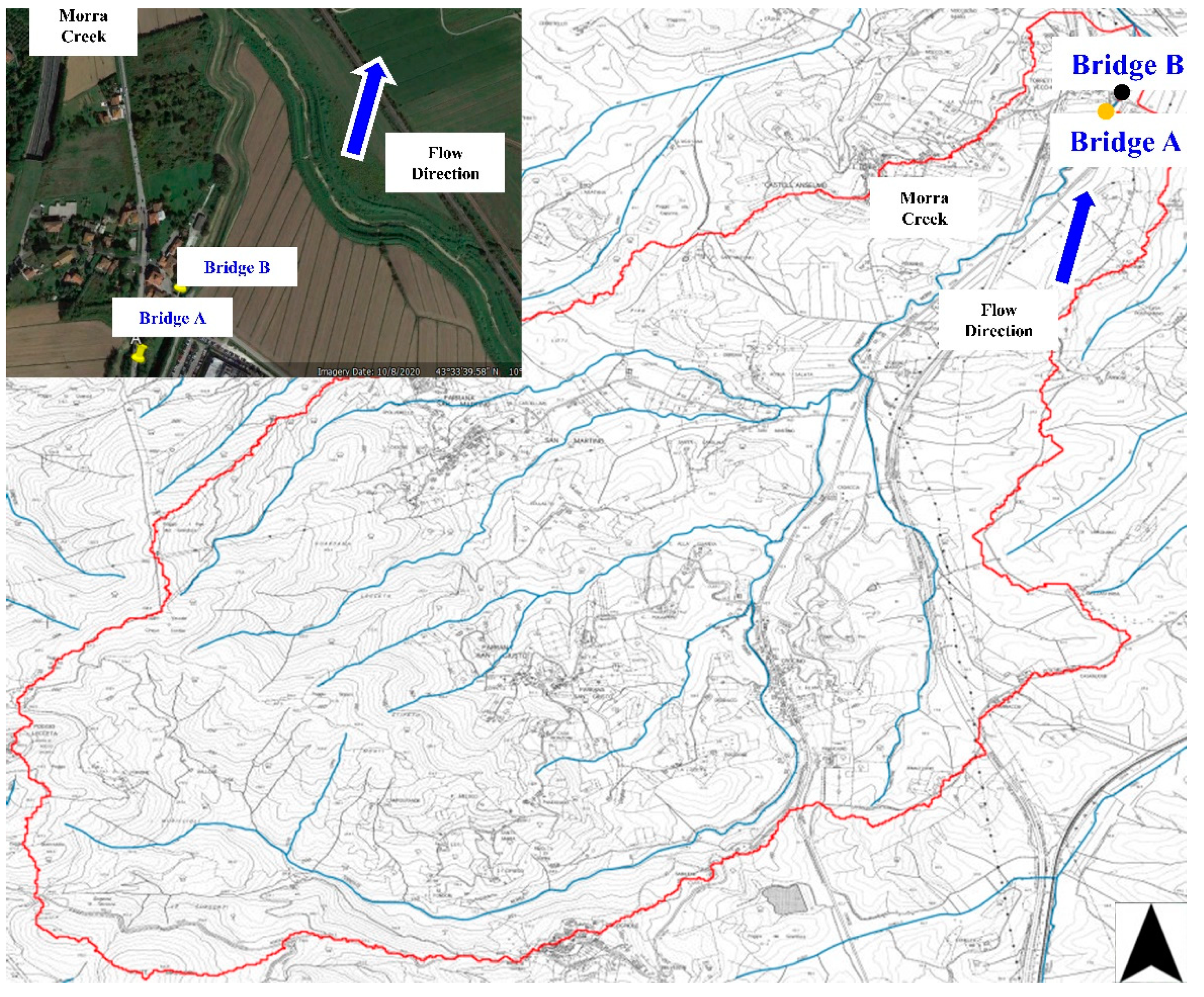
2.1. Study Site
2.2. 1D and 2D Hydraulic Simulations
2.3. Green–blue Flood Control Scenario I
Riverine Vegetation Growth
2.4. Green–Blue Flood Control Scenario II
2.5. Flood Control Efficiency: Peak Discharge and Water Level Reduction
3. Results
3.1. Morra Creek Current Ecohydraulic Conditions
3.2. Green–Blue Flood Control Scenario I
3.3. Green–Blue Flood Control Scenario II
4. Discussion
5. Conclusions
Author Contributions
Funding
Institutional Review Board Statement
Informed Consent Statement
Data Availability Statement
Acknowledgments
Conflicts of Interest
References
- Mazzeo, F.C.; Arienzo, I.; Aulinas, M.; Casalini, M.; Di Renzo, V.; D’Antonio, M. Mineralogical, geochemical and isotopic characteristics of alkaline mafic igneous rocks from Punta delle Pietre Nere (Gargano, Southern Italy). Lithos 2018, 308–309, 316–328. [Google Scholar] [CrossRef]
- Inzunza, D.A.; Montalva, G.A.; Leyton, F.; Prieto, G.; Ruiz, S. Shallow Ambient-Noise 3D Tomography in the Concepción Basin, Chile: Implications for Low-Frequency Ground Motions. Bull. Seism. Soc. Am. 2018, 109, 75–86. [Google Scholar] [CrossRef]
- Santangelo, N.; Forte, G.; De Falco, M.; Chirico, G.B.; Santo, A. New insights on rainfall triggering flow-like landslides and flash floods in Campania (Southern Italy). Landslides 2021, 18, 2923–2933. [Google Scholar] [CrossRef]
- Lama, G.F.C.; Sadeghifar, T.; Torabi Azad, M.; Sihag, P.; Kisi, O. Wind Wave Heights over the Southern Coasts of Caspian Sea: A Real-scale Comparative Analysis. Ocean Eng. 2021. under review. [Google Scholar]
- Fusco, F.; Mirus, B.B.; Baum, R.L.; Calcaterra, D.; De Vita, P. Incorporating the Effects of Complex Soil Layering and Thickness Local Variability into Distributed Landslide Susceptibility Assessments. Water 2021, 13, 713. [Google Scholar] [CrossRef]
- Lama, G.F.C.; Sadeghifar, T.; Sihag, P.; Bayram, A.; Kisi, O. Performance of soft-computing models in predicting wave heights in complex sea flows: Case study of Persian Gulf. Ocean Eng. 2021. under review. [Google Scholar]
- Padulano, R.; Lama, G.F.C.; Rianna, G.; Santini, M.; Mancini, M.; Stojiljkovic, M. Future rainfall scenarios for the assessment of water availability in Italy. In Proceedings of the 2020 IEEE International Workshop on Metrology for Agriculture and Forestry (MetroAgriFor), Trento, Italy, 4–6 November 2020; pp. 241–246. [Google Scholar] [CrossRef]
- Johnston, A.S.A.; Meade, A.; Ardö, J.; Arriga, N.; Black, A.; Blanken, P.D.; Bonal, D.; Brümmer, C.; Cescatti, A.; Dušek, J.; et al. Temperature thresholds of ecosystem respiration at a global scale. Nat. Ecol. Evol. 2021, 5, 487–494. [Google Scholar] [CrossRef] [PubMed]
- Brenna, A.; Surian, N.; Ghinassi, M.; Marchi, L. Sediment–water flows in mountain streams: Recognition and classification based on field evidence. Geomorphology 2020, 371, 107413. [Google Scholar] [CrossRef]
- Manfreda, S.; Miglino, D.; Albertini, C. Impact of detention dams on the probability distribution of floods. Hydrol. Earth Syst. Sci. Discuss. 2021, 25, 4231–4242. [Google Scholar] [CrossRef]
- Francalanci, S.; Paris, E.; Solari, L. On the vulnerability of woody riparian vegetation during flood events. Environ. Fluid Mech. 2020, 20, 635–661. [Google Scholar] [CrossRef]
- Errico, A.; Lama, G.F.C.; Francalanci, S.; Chirico, G.B.; Solari, L.; Preti, F. Flow dynamics and turbulence patterns in a drainage channel colonized by common reed (Phragmites australis) under different scenarios of vegetation management. Ecol. Eng. 2019, 133, 39–52. [Google Scholar] [CrossRef]
- Poggi, D.; Porporato, A.; Ridolfi, R.; Albertson, J.D.; Katul, G.G. The effect of vegetation density on canopy sub-layer turbulence. Bound. Layer Meteorol. 2004, 111, 565–587. [Google Scholar] [CrossRef]
- Västilä, K.; Järvelä, J.; Aberle, J. Characteristic reference areas for estimating flow resistance of natural foliated vegetation. J. Hydrol. 2013, 492, 49–60. [Google Scholar] [CrossRef]
- Bulat, M.; Biron, P.M.; Lacey, J.R.W.; Botrel, M.; Hudon, C.; Maranger, R. A three-dimensional numerical model investigation of the impact of submerged macrophytes on flow dynamics in a large fluvial lake. Freshw. Biol. 2019, 64, 1627–1642. [Google Scholar] [CrossRef]
- Peruzzo, P.; De Serio, F.; Defina, A.; Mossa, M. Wave Height Attenuation and Flow Resistance Due to Emergent or Near-Emergent Vegetation. Water 2018, 10, 402. [Google Scholar] [CrossRef] [Green Version]
- Lama, G.F.C.; Errico, A.; Francalanci, S.; Solari, L.; Preti, F.; Chirico, G.B. Comparative analysis of modeled and measured vegetative Chézy’s flow resistance coefficients in a drainage channel vegetated by dormant riparian reed. In Proceedings of the International IEEE Workshop on Metrology for Agriculture and Forestry, Portici, Italy, 24–26 October 2019; pp. 180–184. [Google Scholar] [CrossRef]
- De Paola, F.; Ranucci, A. Analysis of spatial variability for stormwater capture tank assessment. Irrig. Drain. 2012, 61, 682–690. [Google Scholar] [CrossRef]
- Večeřa, M.; Axmanová, I.; Padullés Cubino, J.; Lososová, Z.; Divíšek, J.; Knollová, I.; Aćić, S.; Biurrun, I.; Boch, S.; Bonari, G.; et al. Mapping species richness of plant families in European vegetation. J. Veg. Sci. 2021, 32, e13035. [Google Scholar] [CrossRef]
- Ferraiuolo, R.; De Paola, F.; Fiorillo, D.; Caroppi, G.; Pugliese, F. Experimental and Numerical Assessment of Water Leakages in a PVC-A Pipe. Water 2020, 12, 1804. [Google Scholar] [CrossRef]
- Chanson, H.; Gualtieri, C. Similitude and scale effects of air entrainment in hydraulic jumps. J. Hydraul. Res. 2008, 46, 35–44. [Google Scholar] [CrossRef] [Green Version]
- Lama, G.F.C.; Errico, A.; Pasquino, V.; Mirzaei, S.; Preti, F.; Chirico, G.B. Velocity Uncertainty Quantification based on Riparian Vegetation Indices in open channels colonized by Phragmites australis. J. Ecohydraulics 2021, 1–6. [Google Scholar] [CrossRef]
- Latella, M.; Bertagni, M.B.; Vezza, P.; Camporeale, C. An integrated methodology to study riparian vegetation dynamics: From field data to impact modeling. J. Adv. Model. Earth Syst. 2020, 12, e2020MS002094. [Google Scholar] [CrossRef] [PubMed]
- Stella, J.C.; Rodríguez-González, P.M.; Dufour, S.; Bendix, J. Riparian vegetation research in Mediterranean-climate regions: Common patterns, ecological processes, and considerations for management. Hydrobiologia 2013, 719, 291–315. [Google Scholar] [CrossRef]
- De Paola, F.; Giugni, M.; Pugliese, F.; Romano, P. Optimal Design of LIDs in Urban Stormwater Systems Using a Harmony-Search Decision Support System. Water Resour. Manag. 2018, 32, 4933–4951. [Google Scholar] [CrossRef]
- Link, O.; Sanhueza, C.; Arriagada, P.; Brevis, W.; Laborde, A.; González, A.; Wilkes, M.; Habit, E. The fish Strouhal number as a criterion for hydraulic fishway design. Ecol. Eng. 2017, 103, 118–126. [Google Scholar] [CrossRef]
- Zou, G.; Papirio, S.; Ylinen, A.; Di Capua, F.; Lakaniemi, A.M.; Puhakka, G.A. Fluidized-bed denitrification for mine waters. Part II: Effects of Ni and Co. Biodegradation 2014, 25, 417–423. [Google Scholar] [CrossRef] [Green Version]
- Pace, R.; De Fino, F.; Rahman, M.A.; Pauleit, S.; Nowak, D.J.; Grote, R. A single tree model to consistently simulate cooling, shading, and pollution uptake of urban trees. Int. J. Biometeorol. 2021, 65, 277–289. [Google Scholar] [CrossRef] [PubMed]
- Bianco, F.; Monteverde, G.; Race, M.; Papirio, S.; Esposito, G. Comparing performances, costs and energy balance of ex situ remediation processes for PAH-contaminated marine sediments. Environ. Sci. Pollut. Res. 2020, 27, 19363–19374. [Google Scholar] [CrossRef]
- Cioffi, B.; Ianiro, G.; Iaccarino, D.; D’Apice, F.; Ferraro, A.; Race, M.; Spasiano, D.; Esposito, E.; Monini, M.; Serra, F.; et al. A potential risk assessment tool to monitor pathogens circulation in coastal waters. Environ. Res. 2021, 200, 111748. [Google Scholar] [CrossRef] [PubMed]
- Licciardello, F.; Sacco, A.; Barbagallo, S.; Ventura, D.; Cirelli, G.L. Evaluation of Different Methods to Assess the Hydraulic Behavior in Horizontal Treatment Wetlands. Water 2020, 12, 2286. [Google Scholar] [CrossRef]
- Varra, G.; Pepe, V.; Cimorelli, L.; Della Morte, R.; Cozzolino, L. On integral and differential porosity models for urban flooding simulation. Adv. Water Resour. 2020, 136, 103455. [Google Scholar] [CrossRef]
- Thiemer, K.; Schneider, S.C.; Demars, B.O.L. Mechanical removal of macrophytes in freshwater ecosystems: Implications for ecosystem structure and function. Sci. Total Environ. 2021, 782, 146671. [Google Scholar] [CrossRef]
- Bonanomi, G.; Zotti, M.; Mogavero, V.; Cesarano, G.; Saulino, L.; Rita, A.; Tesei, G.; Allegrezza, M.; Saracino, A.; Allevato, E. Climatic and anthropogenic factors explain the variability of Fagus sylvatica treeline elevation in fifteen mountain groups across the Apennines. For. Ecosyst. 2020, 7, 5. [Google Scholar] [CrossRef] [Green Version]
- Box, W.; Järvelä, J.; Västilä, K. Flow resistance of floodplain vegetation mixtures for modelling river flows. J. Hydrol. 2021, 601, 126593. [Google Scholar] [CrossRef]
- Artini, G.; Calvani, G.; Francalanci, S.; Solari, L. Effects of vegetation at a bar confluence on river hydrodynamics: The case study of the Arno River at Greve junction. River Res. Appl. 2021, 37, 615–626. [Google Scholar] [CrossRef]
- Peruzzi, C.; Castaldi, M.; Francalanci, S.; Solari, L. Three-dimensional hydraulic characterisation of the Arno River in Florence. J. Flood Risk Manag. 2019, 12, e12490. [Google Scholar] [CrossRef] [Green Version]
- Lama, G.F.C.; Chirico, G.B. Effects of reed beds management on the hydrodynamic behaviour of vegetated open channels. In Proceedings of the 2020 IEEE International Workshop on Metrology for Agriculture and Forestry (MetroAgriFor), Trento, Italy, 4–6 November 2020; pp. 149–154. [Google Scholar] [CrossRef]
- Maji, S.; Hanmaiahgari, P.R.; Balachandar, R.; Pu, J.H.; Ricardo, A.M.; Ferreira, R.M.L. A Review on Hydrodynamics of Free Surface Flows in Emergent Vegetated Channels. Water 2020, 12, 1218. [Google Scholar] [CrossRef]
- Svensk, M.; Coste, S.; Gérard, B.; Gril, E.; Julien, F.; Maillard, P.; Stahl, C.; Leroy, C. Drought effects on resource partition and conservation among leaf ontogenetic stages in epiphytic tank bromeliads. Physiol. Plant. 2020, 170, 488–507. [Google Scholar] [CrossRef] [PubMed]
- Lama, G.F.C.; Crimaldi, M.; Pasquino, V.; Padulano, R.; Chirico, G.B. Bulk Drag Predictions of Riparian Arundo donax Stands through UAV-acquired Multispectral Images. Water 2021, 13, 1333. [Google Scholar] [CrossRef]
- Wang, Y.; Yin, Z.; Liu, Y. Numerical investigation of solitary wave attenuation and resistance induced by rigid vegetation based on a 3-D RANS model. Adv. Water Resour. 2020, 146, 103755. [Google Scholar] [CrossRef]
- van Veelen, T.J.; Karunarathna, H.; Reeve, D.E. Modelling wave attenuation by quasi-flexible coastal vegetation. Coast. Eng. 2021, 164, 103820. [Google Scholar] [CrossRef]
- Del Giudice, G.; Rasulo, G.; Siciliano, D.; Padulano, R. Combined Effects of Parallel and Series Detention Basins for Flood Peak Reduction. Water Resour. Manag. 2014, 28, 3193–3205. [Google Scholar] [CrossRef]
- Liu, C.; Shan, Y. Analytical model for predicting the longitudinal profiles of velocities in a channel with a model vegetation patch. J. Hydrol. 2019, 576, 561–574. [Google Scholar] [CrossRef]
- Lama, G.F.C.; Errico, A.; Francalanci, S.; Solari, L.; Preti, F.; Chirico, G.B. Evaluation of Flow Resistance Models Based on Field Experiments in a Partly Vegetated Reclamation Channel. Geosciences 2020, 10, 47. [Google Scholar] [CrossRef] [Green Version]
- West, P.O.; Wallis, S.G.; Sonnenwald, F.C.; Hart, J.R.; Stovin, V.R.; Guymer, I. Modelling transverse solute mixing across a vegetation generated shear layer. J. Hydraul. Res. 2020, 59, 621–636. [Google Scholar] [CrossRef]
- Zhu, Z.; Yang, Z.; Huai, W.; Wang, H.; Li, D.; Fan, Y. Growth-decay model of vegetation based on hydrodynamics and simulation on vegetation evolution in the channel. Ecol. Indic. 2020, 119, 106857. [Google Scholar] [CrossRef]
- Di Cristo, C.; Iervolino, M.; Vacca, A. Applicability of Kinematic and Diffusive models for mud-flows: A steady state analysis. J. Hydrol. 2018, 559, 585–595. [Google Scholar] [CrossRef]
- Di Nunno, F.; Granata, F.; Gargano, R.; De Marinis, G. Prediction of spring flows using nonlinear autoregressive exogenous (NARX) neural network models. Environ. Monit. Assess. 2021, 193, 350. [Google Scholar] [CrossRef]
- Gobbetti, L.E.C. Design of the filling and emptying system of the new Panama Canal locks. J. Appl. Water Eng. Res. 2013, 1, 28–38. [Google Scholar] [CrossRef]
- Fecarotta, O.; Messa, G.V.; Pugliese, F. Numerical assessment of the vulnerability to impact erosion of a pump as turbine in a water supply system. J. Hydroinform. 2020, 22, 691–712. [Google Scholar] [CrossRef]
- Badas, M.G.; Rossi, R.; Garau, M. May a Standard VOF Numerical Simulation Adequately Complete Spillway Laboratory Measurements in an Operational Context? The Case of Sa Stria Dam. Water 2020, 12, 1606. [Google Scholar] [CrossRef]
- Nicolosi, F.; Ciliberti, D.; Della Vecchia, P.; Corcione, S. Experimental analysis of aircraft directional control effectiveness. Aerosp. Sci. Technol. 2020, 106, 106099. [Google Scholar] [CrossRef]
- Lama, G.F.C.; Crimaldi, M. Calibration of Flow Resistance Models in Vegetated Ditches Based on UAV Remote Sensing. Presented at the 1st International Electronic Conference on Agronomy, online, 3–17 May 2021; Volume 3, pp. 17–21. [Google Scholar]
- Eke, E.; Czapiga, M.; Viparelli, E.; Shimizu, Y.; Imran, J.; Sun, T.; Parker, G. Coevolution of width and sinuosity in meandering rivers. J. Fluid Mech. 2014, 760, 127–174. [Google Scholar] [CrossRef]
- Vettori, D.; Nikora, V. Flow–seaweed interactions: A laboratory study using blade models. Environ. Fluid Mech. 2018, 18, 611–636. [Google Scholar] [CrossRef] [Green Version]
- Bahmanpouri, F.; Daliri, M.; Khoshkonesh, A.; Namin, M.M.; Buccino, M. Bed compaction effect on dam break flow over erodible bed; experimental and numerical modeling. J. Hydrol. 2020, 594, 125645. [Google Scholar] [CrossRef]
- Di Cristo, C.; Iervolino, M.; Moramarco, T.; Vacca, A. Applicability of Diffusive model for mud-flows: An unsteady analysis. J. Hydrol. 2021, 600, 126512. [Google Scholar] [CrossRef]
- Sarghini, F.; De Vivo, A. Analysis of preliminary design requirements of a heavy lift Multirotor drone for agricultural use. Chem. Eng. Trans. 2017, 58, 625–630. [Google Scholar] [CrossRef]
- Modarelli, G.C.; Arena, C.; Pesce, G.; Dell’Aversana, E.; Fusco, G.M.; Carillo, P.; De Pascale, S.; Paradiso, R. The role of light quality of photoperiodic lighting on photosynthesis, flowering and metabolic profiling in Ranunculus asiaticus L. Physiol. Plant. 2020, 170, 187–201. [Google Scholar] [CrossRef] [PubMed]
- Cristofano, F.; El-Nakhel, C.; Rouphael, Y. Biostimulant Substances for Sustainable Agriculture: Origin, Operating Mechanisms and Effects on Cucurbits, Leafy Greens, and Nightshade Vegetables Species. Biomolecules 2021, 11, 1103. [Google Scholar] [CrossRef] [PubMed]
- Crimaldi, M.; Lama, G.F.C. Impacts of riparian plants biomass assessed by UAV-acquired multispectral images on the hydrodynamics of vegetated streams. In Proceedings of the 29th European Biomass Conference and Exhibition, online, 26–29 April 2021; pp. 1157–1161. [Google Scholar] [CrossRef]
- Aliberti, A.; Olivieri, F.; Graci, S.; Rigano, M.M.; Barone, A.; Ruggieri, V. Genomic Dissection of a Wild Region in a Superior Solanum pennellii Introgression Sub-Line with High Ascorbic Acid Accumulation in Tomato Fruit. Genes 2020, 11, 847. [Google Scholar] [CrossRef]
- Lama, G.F.C.; Crimaldi, M. Assessing the role of Gap Fraction on the Leaf Area Index (LAI) estimations of riparian vegetation based on Fisheye lenses. In Proceedings of the 29th European Biomass Conference and Exhibition, online, 26–29 April 2021; pp. 1172–1176. [Google Scholar] [CrossRef]
- Modarelli, G.C.; Rouphael, Y.; De Pascale, S.; Öztekin, G.B.; Tüzel, Y.; Orsini, F.; Gianquinto, G. Appraisal of Salt Tolerance under Greenhouse Conditions of a Cucurbitaceae Genetic Repository of Potential Rootstocks and Scions. Agronomy 2020, 10, 967. [Google Scholar] [CrossRef]
- Olivieri, F.; Calafiore, R.; Francesca, S.; Schettini, C.; Chiaiese, P.; Rigano, M.M.; Barone, A. High-Throughput Genotyping of Resilient Tomato Landraces to Detect Candidate Genes Involved in the Response to High Temperatures. Genes 2020, 11, 626. [Google Scholar] [CrossRef] [PubMed]
- Lama, G.F.C.; Errico, A.; Francalanci, S.; Solari, L.; Chirico, G.B.; Preti, F. Hydraulic Modeling of Field Experiments in a Drainage Channel Under Different Riparian Vegetation Scenarios. In Innovative Biosystems Engineering for Sustainable Agriculture, Forestry and Food Production; Coppola, A., Di Renzo, G., Altieri, G., D’Antonio, P., Eds.; Springer: Cham, Switzerland, 2020; pp. 69–77. [Google Scholar] [CrossRef]
- Capolupo, A.; Kooistra, L.; Berendonk, C.; Boccia, L.; Suomalainen, J. Estimating Plant Traits of Grasslands from UAV-Acquired Hyperspectral Images: A Comparison of Statistical Approaches. ISPRS Int. J. Geo-Inf. 2015, 4, 2792–2820. [Google Scholar] [CrossRef]
- Fecarotta, O.; Martino, R.; Morani, M.C. Wastewater Pump Control under Mechanical Wear. Water 2019, 11, 1210. [Google Scholar] [CrossRef] [Green Version]
- Forzieri, G.; Guarnieri, L.; Vivoni, E.R.; Castelli, F.; Preti, F. Spectral-ALS data fusion for different roughness parameterizations of forested floodplains. River Res. Applic. 2011, 27, 826–840. [Google Scholar] [CrossRef]
- Piemontese, L.; Castelli, G.; Fetzer, I.; Barron, J.; Liniger, H.; Harari, N.; Bresci, E.; Jaramillo, F. Estimating the global potential of water harvesting from successful case studies. Glob. Environ. Chang. 2020, 63, 10212. [Google Scholar] [CrossRef]
- Liu, D.; Valyrakis, M.; Williams, R. Flow Hydrodynamics across Open Channel Flows with Riparian Zones: Implications for Riverbank Stability. Water 2017, 9, 720. [Google Scholar] [CrossRef] [Green Version]
- Padulano, R.; Rianna, G.; Santini, M. Datasets and approaches for the estimation of rainfall erosivity over Italy: A comprehensive comparison study and a new method. J. Hydrol. Reg. Stud. 2021, 34, 100788. [Google Scholar] [CrossRef]
- Nuzzo, A.; Buurman, P.; Cozzolino, V.; Spaccini, R.; Picoolo, A. Infrared spectra of soil organic matter under a primary vegetation sequence. Chem. Biol. Technol. Agric. 2020, 7, 6. [Google Scholar] [CrossRef] [Green Version]
- Qiu, J.; Cao, B.; Park, E.; Yang, X.; Zhang, W.; Tarolli, P. Flood Monitoring in Rural Areas of the Pearl River Basin (China) Using Sentinel-1 SAR. Remote Sens. 2021, 13, 1384. [Google Scholar] [CrossRef]


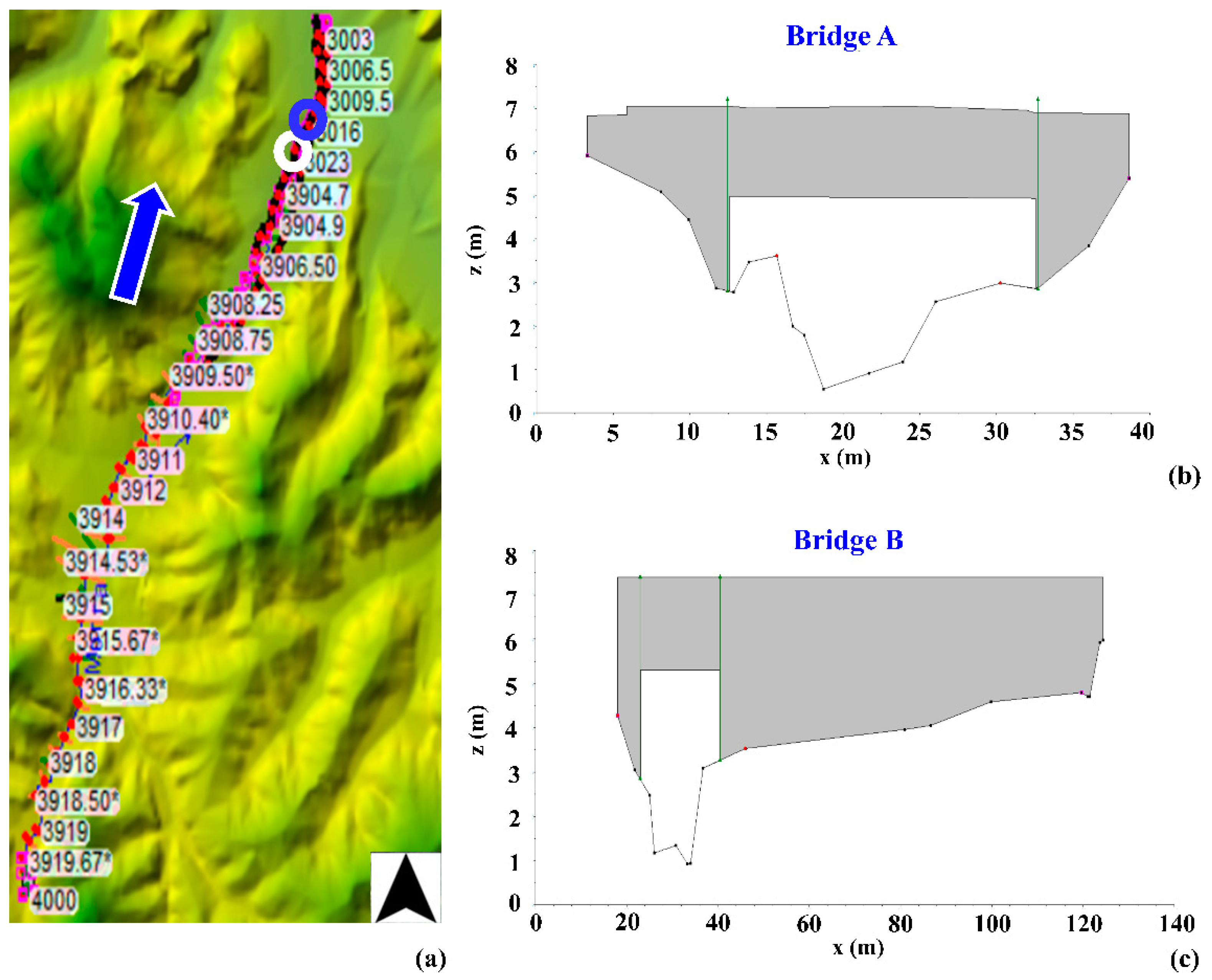
| Span Features | Dimensions (m) |
|---|---|
| Height | 4.40 |
| Width | 18.55 |
| Length | 10.38 |
| Span Features | Dimensions (m) |
|---|---|
| Height | 4.50 |
| Width | 8.07 |
| Length | 5.23 |
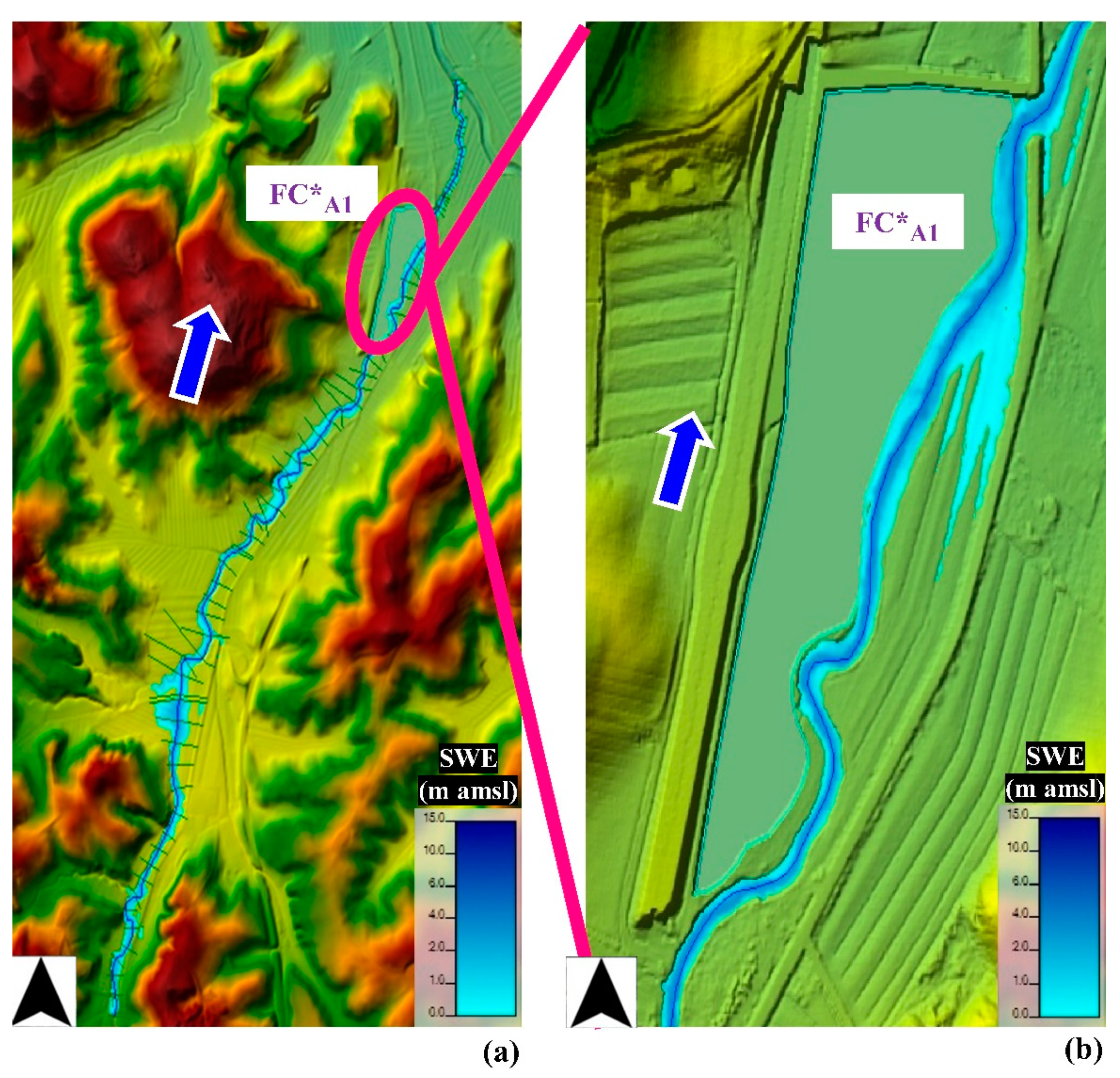
| FC*A1 Feature | Value |
|---|---|
| Volume (m3) | 8.02 × 10³ |
| Depth (m) | 1.26 |
| Length (m) | 730 |
| Width (m) | 105 |
| Scenario | Scheme | Runs |
|---|---|---|
| Current ecohydraulic conditions | 1D | 1 |
| Green–blue scenario I | 1D | 20 |
| Green–blue scenario II | 1D + 2D (2 areas) | 1 |
| 1D + 2D (1 area) | 1 |
| t (h) | QII (m3 s−1) | hII (m) |
|---|---|---|
| 0 | 3.41 | 1.03 |
| 1 | 9.32 | 1.64 |
| 2 | 68.47 | 2.76 |
| 3 | 109.53 | 4.04 |
| 4 | 97.14 | 3.93 |
| 5 | 40.66 | 2.39 |
| 6 | 17.39 | 2.05 |
| 7 | 9.22 | 1.99 |
| 8 | 4.68 | 1.01 |
Publisher’s Note: MDPI stays neutral with regard to jurisdictional claims in published maps and institutional affiliations. |
© 2021 by the authors. Licensee MDPI, Basel, Switzerland. This article is an open access article distributed under the terms and conditions of the Creative Commons Attribution (CC BY) license (https://creativecommons.org/licenses/by/4.0/).
Share and Cite
Lama, G.F.C.; Rillo Migliorini Giovannini, M.; Errico, A.; Mirzaei, S.; Padulano, R.; Chirico, G.B.; Preti, F. Hydraulic Efficiency of Green-Blue Flood Control Scenarios for Vegetated Rivers: 1D and 2D Unsteady Simulations. Water 2021, 13, 2620. https://doi.org/10.3390/w13192620
Lama GFC, Rillo Migliorini Giovannini M, Errico A, Mirzaei S, Padulano R, Chirico GB, Preti F. Hydraulic Efficiency of Green-Blue Flood Control Scenarios for Vegetated Rivers: 1D and 2D Unsteady Simulations. Water. 2021; 13(19):2620. https://doi.org/10.3390/w13192620
Chicago/Turabian StyleLama, Giuseppe Francesco Cesare, Matteo Rillo Migliorini Giovannini, Alessandro Errico, Sajjad Mirzaei, Roberta Padulano, Giovanni Battista Chirico, and Federico Preti. 2021. "Hydraulic Efficiency of Green-Blue Flood Control Scenarios for Vegetated Rivers: 1D and 2D Unsteady Simulations" Water 13, no. 19: 2620. https://doi.org/10.3390/w13192620