
Multi-Scale Analysis of the Dependence of Water Quality on Land Use Using Linear and Mixed Models


Abstract
:1. Introduction
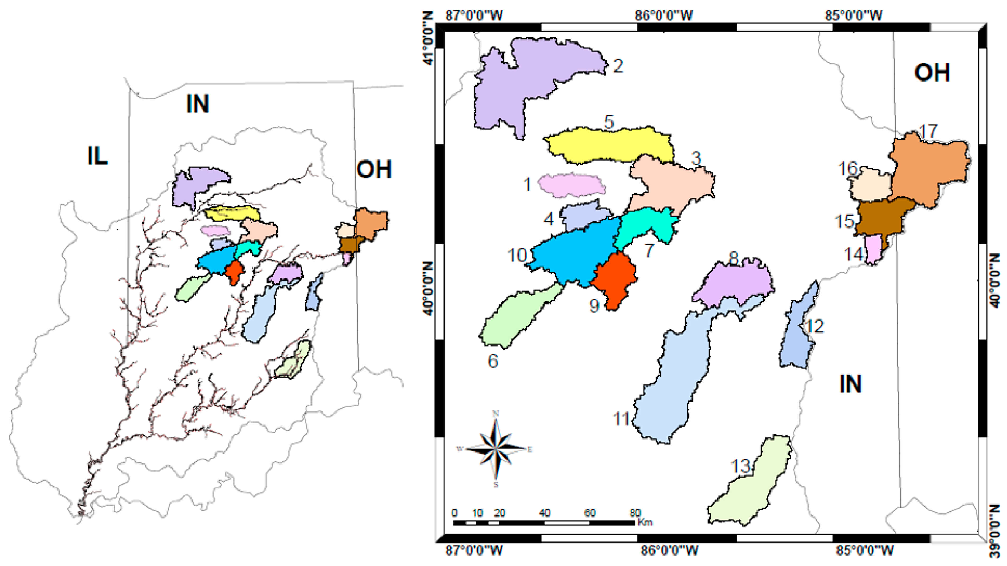
2. Study Area
2.1. Watershed Characteristics
2.2. Data
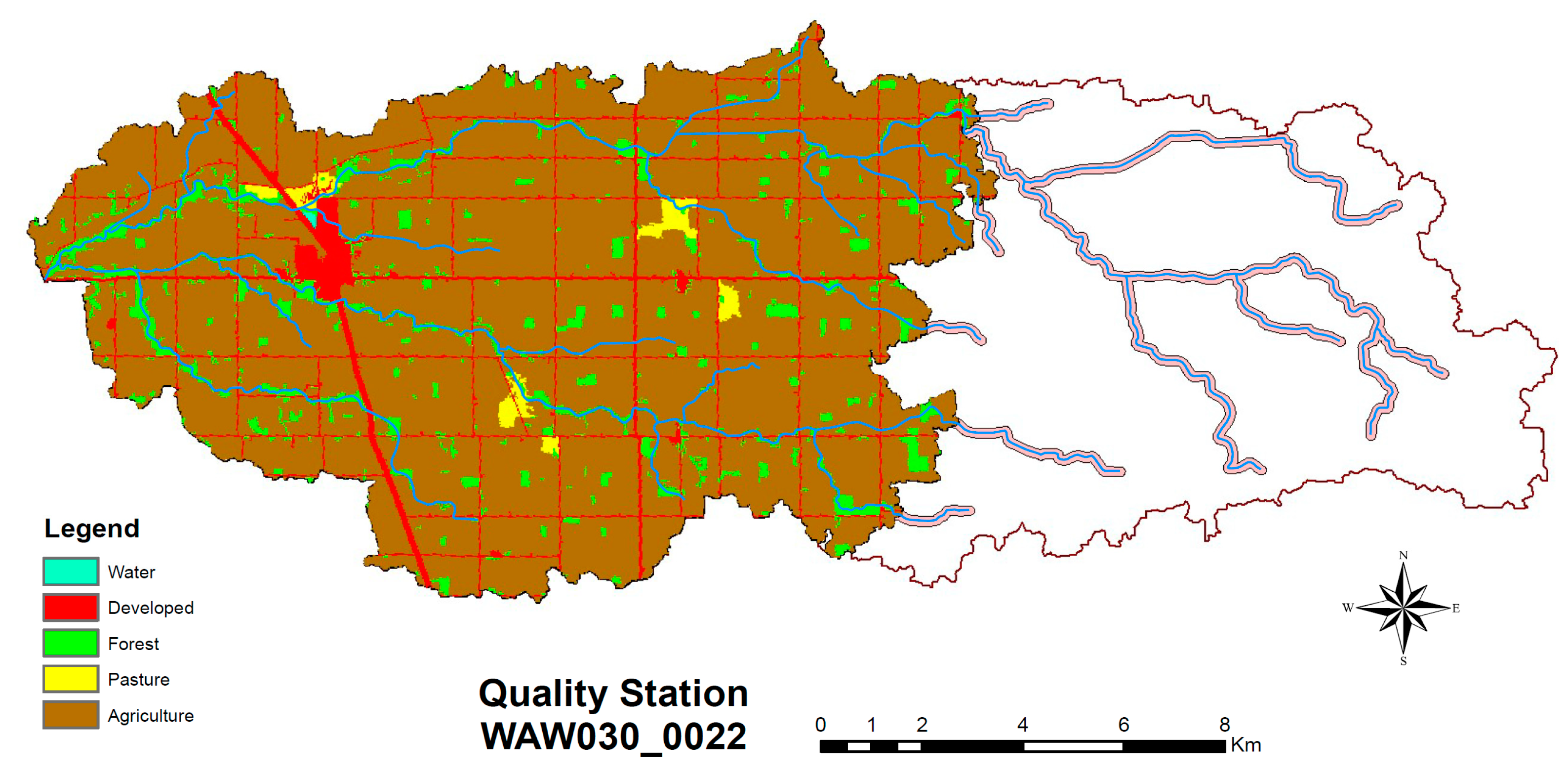
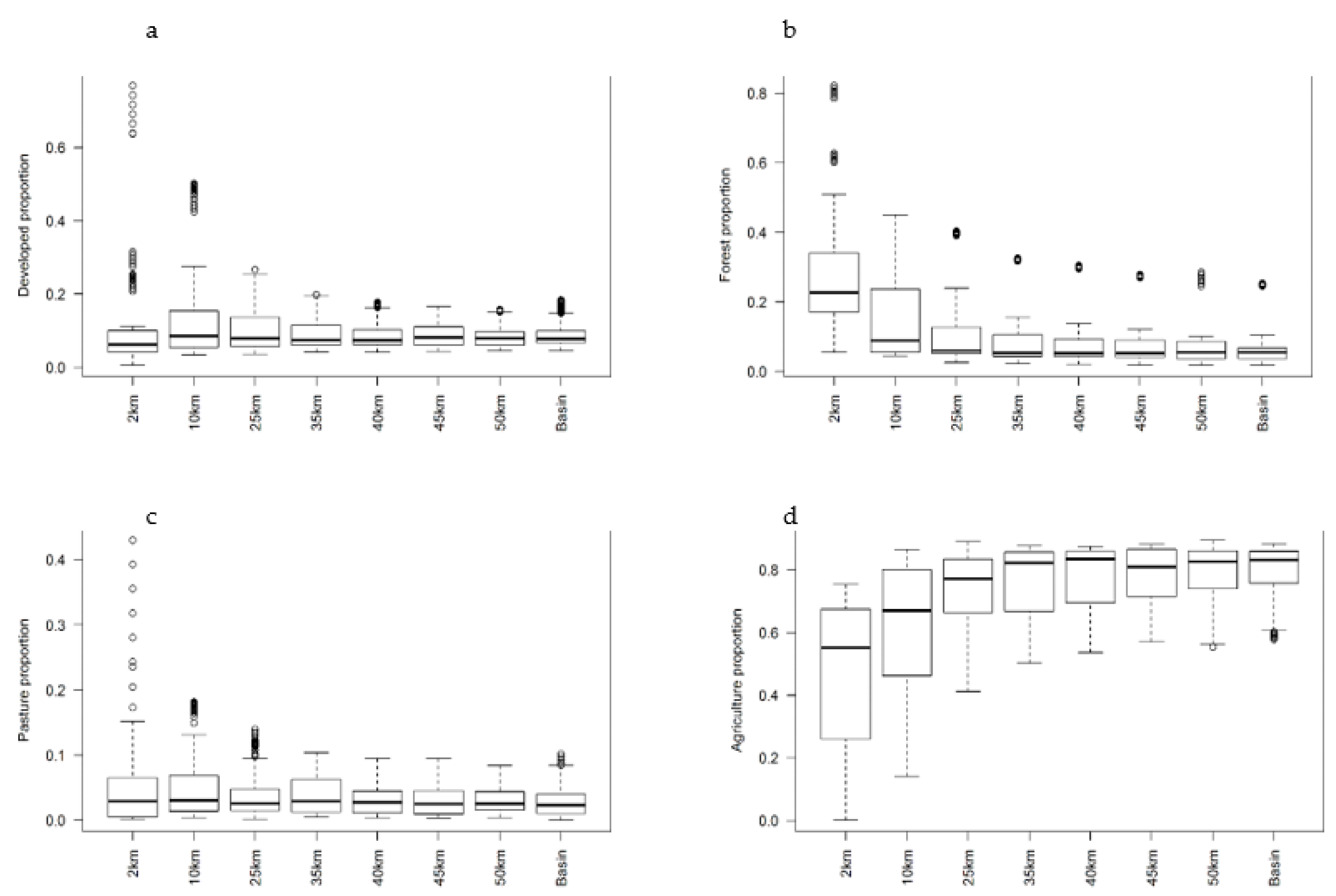
2.3. Spatial Analysis
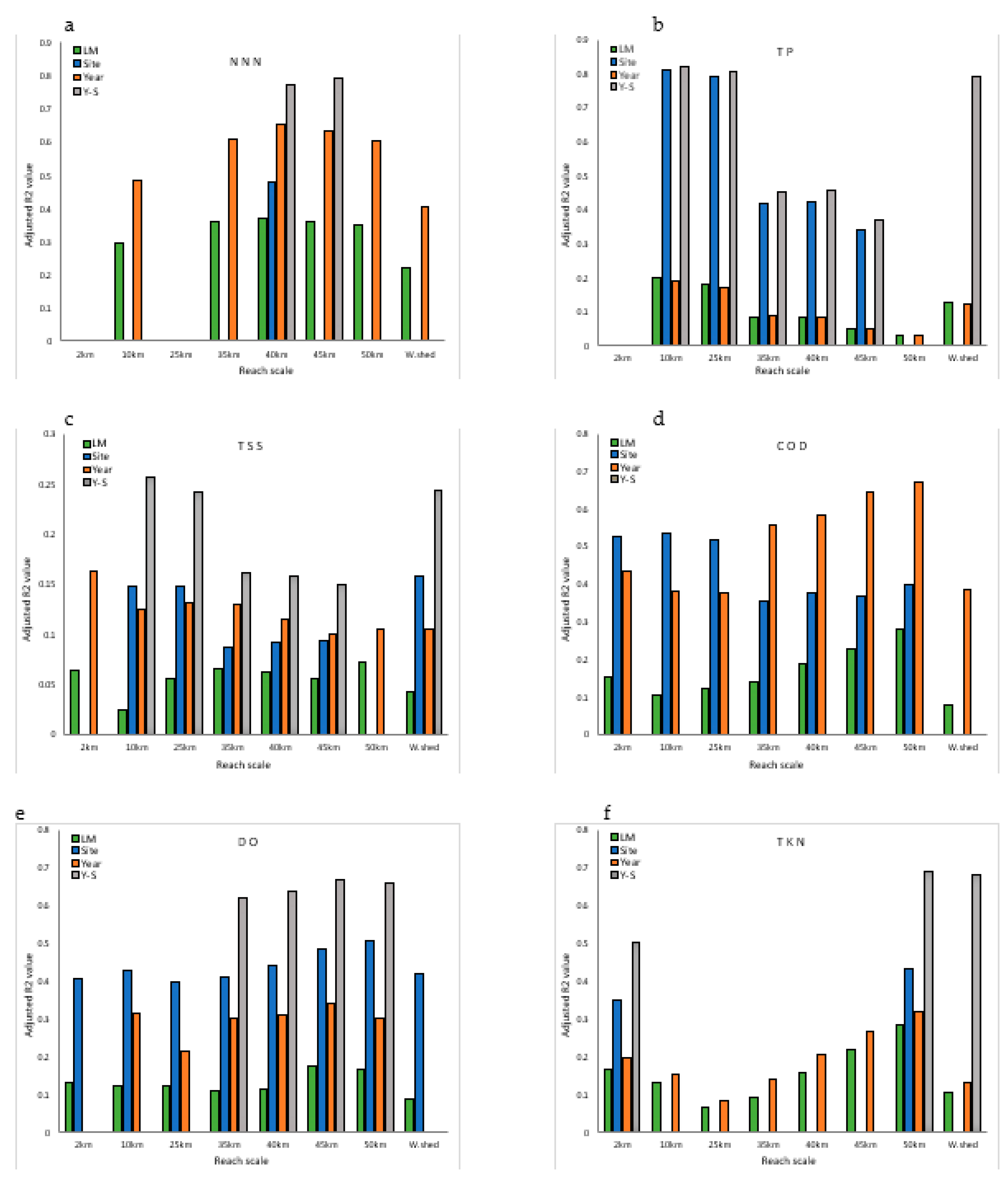
2.4. Statistical Analysis
3. Results and Discussion
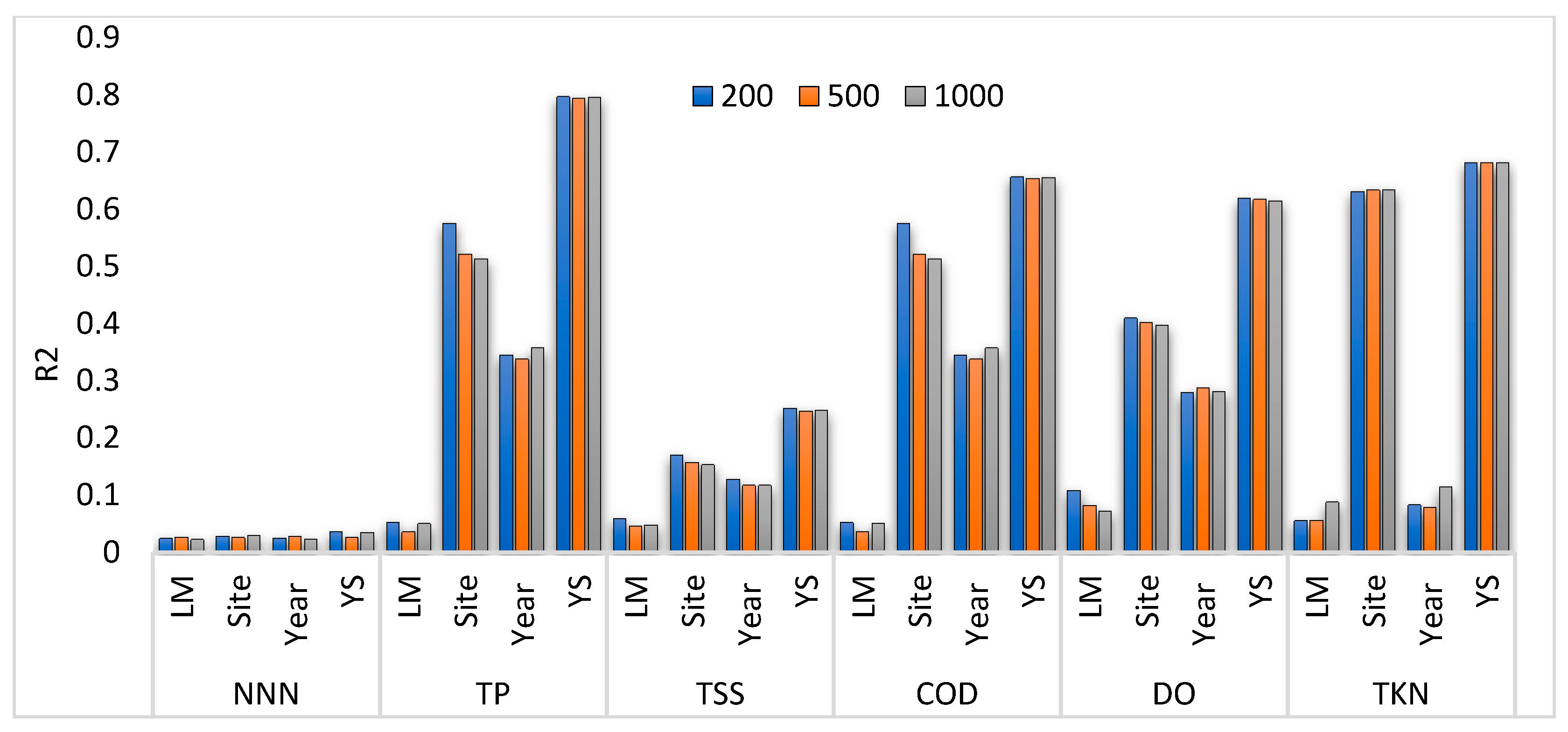
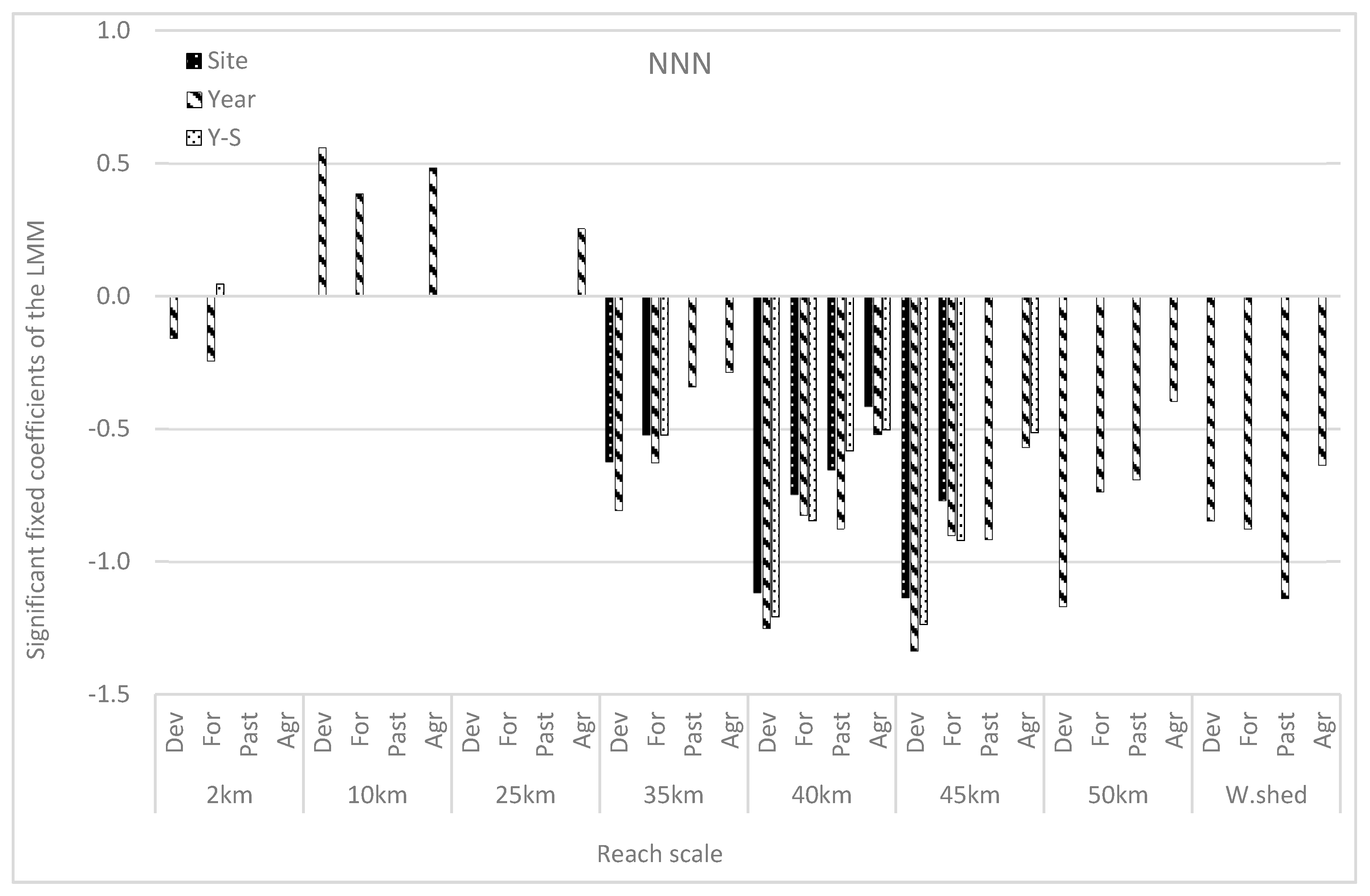
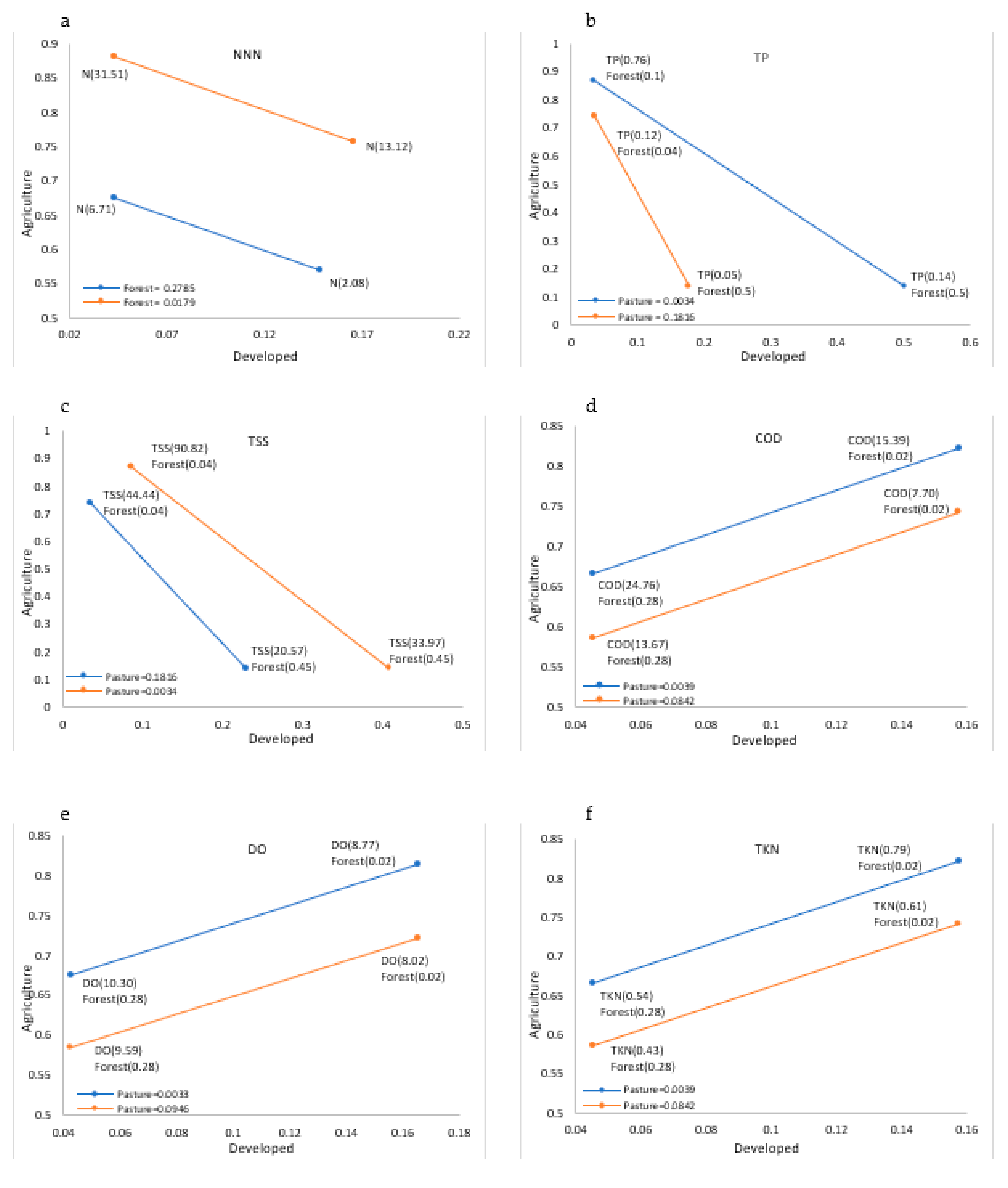
Relationship between Land Use and Water Quality
4. Conclusions
Supplementary Materials
Author Contributions
Funding
Data Availability Statement
Acknowledgments
Conflicts of Interest
References
- Haidary, A.; Amiri, B.J.; Adamowski, J.; Fohrer, N.; Nakane, K. Assessing the impacts of four land use types on the water quality of wetlands in Japan. Water Resour. Manag. 2013, 27, 2217–2229. [Google Scholar] [CrossRef]
- Tong, S.; Chen, W. Modeling the relationship between land use and surface water quality. J. Environ. Manag. 2002, 66, 377–393. [Google Scholar] [CrossRef] [PubMed]
- Aboelnour, M.; Gitau, M.W.; Engel, B.A. Hydrologic response in an urban watershed as affected by climate and land-use change. Water 2019, 11, 1603. [Google Scholar] [CrossRef] [Green Version]
- Meynendonckx, J.; Heuvelmans, G.; Muys, B.; Feyen, J. Hydrology and earth system sciences effects of watershed and riparian zone characteristics on nutrient concentrations in the River Scheldt Basin. PLoS ONE 2006, 10, e53163. [Google Scholar] [CrossRef]
- Tromboni, F.; Dilts, T.E.; Null, S.E.; Lohani, S.; Ngor, P.B.; Soum, S.; Hogan, Z.; Chandra, S. Changing land use and population density are degrading water quality in the lower mekong basin. Water 2021, 13, 1948. [Google Scholar] [CrossRef]
- Wilson, C.; Weng, Q. Assessing surface water quality and its relation with urban land cover changes in the Lake Calumet Area, Greater Chicago. Environ. Manag. 2010, 45, 1096–1111. [Google Scholar] [CrossRef] [PubMed]
- Mander, Ü.; Kull, A.; Tamm, V.; Kuusemets, V.; Karjus, R. Impact of climatic fluctuations and land use change on runoff and nutrient losses in rural landscapes. Landsc. Urban Plan. 1998, 41, 229–238. [Google Scholar] [CrossRef]
- Aboelnour, M.; Engel, B.A. Application of remote sensing techniques and geographic information systems to analyze land surface temperature in response to land use/land cover change in greater Cairo Region, Egypt. J. Geogr. Inf. Syst. 2018, 10, 57–88. [Google Scholar] [CrossRef] [Green Version]
- Baker, T.J.; Miller, S.N. Using the soil and water assessment tool (SWAT) to assess land use impact on water resources in an East African watershed. J. Hydrol. 2013, 486, 100–111. [Google Scholar] [CrossRef]
- Alberti, M.; Booth, D.; Hill, K.; Coburn, B.; Avolio, C.; Coe, S.; Spirandelli, D. The impact of urban patterns on aquatic ecosystems: An empirical analysis in Puget lowland sub-basins. Landsc. Urban Plan. 2007, 80, 345–361. [Google Scholar] [CrossRef]
- King, R.S.; Baker, M.E.; Whigham, D.F.; Weller, D.E.; Jordan, T.E.; Kazyak, P.F.; Hurd, M.K. Spatial considerations for linking watershed land cover to ecological indicators in streams. Ecol. Appl. 2005, 15, 137–153. [Google Scholar] [CrossRef] [Green Version]
- Shi, P.; Zhang, Y.; Li, Z.; Li, P.; Xu, G. Influence of land use and land cover patterns on seasonal water quality at multi-spatial scales. Catena 2017, 151, 182–190. [Google Scholar] [CrossRef]
- Woli, K.P.; Nagumo, T.; Kuramochi, K.; Hatano, R. Evaluating river water quality through land use analysis and N budget approaches in livestock farming areas. Sci. Total Environ. 2004, 329, 61–74. [Google Scholar] [CrossRef] [Green Version]
- Amiri, B.; Nakane, K. Entire catchment and buffer zone approaches to modeling linkage between river water quality and land cover-a case study of Yamaguchi Prefecture, Japan. Chin. Geogr. Sci. 2008, 18, 85–92. [Google Scholar] [CrossRef] [Green Version]
- Shen, Z.; Hou, X.; Li, W.; Aini, G.; Chen, L.; Gong, Y. Impact of landscape pattern at multiple spatial scales on water quality: A case study in a typical urbanised watershed in China. Ecol. Indic. 2015, 48, 417–427. [Google Scholar] [CrossRef]
- Uriarte, M.; Yackulic, C.B.; Lim, Y.; Arce-Nazario, J.A. Influence of land use on water quality in a tropical landscape: A multi-scale analysis. Landsc. Ecol. 2011, 26, 1151–1164. [Google Scholar] [CrossRef] [Green Version]
- Gamvroula, D.; Alexakis, D.; Stamatis, G. Diagnosis of groundwater quality and assessment of contamination sources in the Megara basin (Attica, Greece). Arab. J. Geosci. 2013, 6, 2367–2381. [Google Scholar] [CrossRef]
- Huang, J.; Zhan, J.; Yan, H.; Wu, F.; Deng, X. Evaluation of the impacts of land use on water quality: A case study in the Chaohu lake basin. Sci. World J. 2013, 2013, 329187. [Google Scholar] [CrossRef] [Green Version]
- Zhang, S.; Fan, W.; Li, Y.; Yi, Y. The influence of changes in land use and landscape patterns on soil erosion in a watershed. Sci. Total Environ. 2017, 574, 34–45. [Google Scholar] [CrossRef] [PubMed]
- Alexakis, D.E.; Bathrellos, G.D.; Skilodimou, H.D.; Gamvroula, D.E. Land suitability mapping using geochemical and spatial analysis methods. Appl. Sci. 2021, 11, 5404. [Google Scholar] [CrossRef]
- Ma, X.; Xu, J.; Luo, Y.; Prasad Aggarwal, S.; Li, J. Response of hydrological processes to land-cover and climate changes in Kejie watershed, south-west China. Hydrol. Process. 2009, 23, 1179–1191. [Google Scholar] [CrossRef]
- Ding, J.; Jiang, Y.; Liu, Q.; Hou, Z.; Liao, J.; Fu, L.; Peng, Q. Influences of the land use pattern on water quality in low-order streams of the Dongjiang River basin, China: A multi-scale analysis. Sci. Total Environ. 2016, 551–552, 205–216. [Google Scholar] [CrossRef]
- Sun, Y.; Guo, Q.; Liu, J.; Wang, R. Scale effects on spatially varying relationships between urban landscape patterns and water quality. Environ. Manag. 2014, 54, 272–287. [Google Scholar] [CrossRef] [PubMed]
- Allan, D. Landscapes and riverscapes: The influence of land use on stream ecosystems. Annu. Rev. Ecol. Evol. Syst. 2004, 35, 257–284. [Google Scholar] [CrossRef] [Green Version]
- Pratt, B.; Chang, H. Effects of land cover, topography, and built structure on seasonal water quality at multiple spatial scales. J. Hazard. Mater. 2012, 209–210, 48–58. [Google Scholar] [CrossRef]
- Schilling, K.E.; Jha, M.K.; Zhang, Y.K.; Gassman, P.W.; Wolter, C.F. Impact of land use and land cover change on the water balance of a large agricultural watershed: Historical effects and future directions. Water Resour. Res. 2008, 45. [Google Scholar] [CrossRef]
- Williams, M.R.; King, K.W.; Macrae, M.L.; Ford, W.; Van Esbroeck, C.; Brunke, R.I.; English, M.C.; Schiff, S.L. Uncertainty in nutrient loads from tile-drained landscapes: Effect of sampling frequency, calculation algorithm, and compositing strategy. J. Hydrol. 2015, 530, 306–316. [Google Scholar] [CrossRef]
- Collins, K.E.; Doscher, C.; Rennie, H.G.; Ross, J.G. The effectiveness of Riparian ‘Restoration’ on water quality-a case study of Lowland Streams in Canterbury, New Zealand. Restor. Ecol. 2013, 21, 40–48. [Google Scholar] [CrossRef]
- McMillan, S.K.; Tuttle, A.K.; Jennings, G.D.; Gardner, A. Influence of restoration age and Riparian vegetation on reach-scale nutrient retention in restored urban streams. JAWRA J. Am. Water Resour. Assoc. 2014, 50, 626–638. [Google Scholar] [CrossRef]
- Sahu, M.; Gu, R.R. Modeling the effects of riparian buffer zone and contour strips on stream water quality. Ecol. Eng. 2009, 35, 1167–1177. [Google Scholar] [CrossRef]
- Peterson, F.; Risberg, J. Nutrients: Phosphorus, Nitrogen Sources, Impact on Water Quality-A General Overview; Minnesota Pollution Control Agency: Saint Paul, MN, USA, 2008. [Google Scholar]
- Chappell, N.A.; Jones, T.D.; Tych, W. Sampling frequency for water quality variables in streams: Systems analysis to quantify minimum monitoring rates. Water Res. 2017, 123, 49–57. [Google Scholar] [CrossRef] [PubMed]
- Kumar, M.; Puri, A. A review of permissible limits of drinking water. Indian J. Occup. Environ. Med. 2012, 16, 40–44. [Google Scholar] [CrossRef] [PubMed] [Green Version]
- Teixeira, Z.; Marques, J.C. Relating landscape to stream nitrate-N levels in a coastal eastern-Atlantic watershed (Portugal). Ecol. Indic. 2015, 61, 149–1056. [Google Scholar] [CrossRef]
- Pyron, M.; Neumann, K. Hydrologic alterations in the Wabash River watershed, USA. River Res. Appl. 2008, 24, 1175–1184. [Google Scholar] [CrossRef]
- Gammon, J. The Wabash River Ecosystem; Cinergy Corporation: Cincinnati, OH, USA, 1998; ISBN 0253212723. [Google Scholar]
- White, D.; Johnston, K.; Miller, M. Ohio River Basin; Academic Press: Cambridge, MA, USA, 2005. [Google Scholar]
- Gammon, J. The status of riparian wetlands in west-central Indiana streams. Proc. Indiana Acad. Sci. 1994, 103, 195–214. [Google Scholar]
- Bonansea, M.; Rodriguez, M.C.; Pinotti, L.; Ferrero, S. Using multi-temporal Landsat imagery and linear mixed models for assessing water quality parameters in Río Tercero reservoir (Argentina). Remote Sens. Environ. 2015, 158, 28–41. [Google Scholar] [CrossRef]
- Lark, R.M.; Cullis, B.R. Model-based analysis using REML for inference from systematically sampled data on soil. Eur. J. Soil Sci. 2004, 55, 799–813. [Google Scholar] [CrossRef]
- Lessels, J.S.; Bishop, T.F.A. Estimating water quality using linear mixed models with stream discharge and turbidity. J. Hydrol. 2013, 498, 13–22. [Google Scholar] [CrossRef]
- Buck, O.; Niyogi, D.K.; Townsend, C.R. Scale-dependence of land use effects on water quality of streams in agricultural catchments. Environ. Pollut. 2004, 130, 287–299. [Google Scholar] [CrossRef]
- Kumar, S.; Merwade, V.; Kam, J.; Thurner, K. Streamflow trends in Indiana: Effects of long term persistence, precipitation and subsurface drains. J. Hydrol. 2009, 374, 171–183. [Google Scholar] [CrossRef]
- Karns, D.R.; Pyron, M.; Simon, T.P. Proceedings of the Indiana Academy of Science; St. Mary-of-the-Woods College: Arlington, IN, USA, 2006; Volume 1. [Google Scholar]
- Multi-Resolution Land Characteristics (MRLC) Consortium|Multi-Resolution Land Characteristics (MRLC) Consortium. Available online: https://www.mrlc.gov/ (accessed on 11 May 2020).
- Schmadel, N.M.; Harvey, J.W. NHD Plus; USGS: Reston, VA, USA, 2020. [Google Scholar]
- Nejadhashemi, A.P.; Shen, C.; Associate, R.; Wardynski, B.J.; Assistant, R.; Mantha, P.S.; Lawrence, D.L. Evaluating the Impacts of Land Use Changes on Hydrologic Responses in the Agricultural Regions of Michigan and Wisconsin. In Proceedings of the 2010 ASABE Annual International Meeting Sponsored by ASABE, Pittsburgh, PA, USA, 20–23 January 2010. [Google Scholar]
- US EPA. Water Quality Data (WQX); U.S. Environmental Protection Agency: Virginia, DC, USA, 2017. [Google Scholar]
- O’Callaghan, J.F.; Mark, D.M. The extraction of drainage networks from digital elevation data. Comput. Vision Graph. Image Process. 1984, 28, 323–344. [Google Scholar] [CrossRef]
- Jenson, S.K.; Domingue, J.O. Extracting topographic structure from digital elevation data for geographic information system analysis. Photogramm. Eng. Remote Sens. 1988, 54, 1593–1600. [Google Scholar]
- Basu, N.B.; Destouni, G.; Jawitz, J.W.; Thompson, S.E.; Loukinova, N.V.; Darracq, A.; Zanardo, S.; Yaeger, M.; Sivapalan, M.; Rinaldo, A.; et al. Nutrient loads exported from managed catchments reveal emergent biogeochemical stationarity. Geophys. Res. Lett. 2010, 37, L23404. [Google Scholar] [CrossRef]
- Legendre, P.; Legendre, L. Numerical Ecology Ch 6-Multidimensional qualitative data. Dev. Environ. Model. 2012, 24, 337–424. [Google Scholar] [CrossRef]
- Bring, J. How to standardize regression coefficients. Am. Stat. 1994, 48, 209–213. [Google Scholar] [CrossRef]
- McDonald, J.H. Handbook of Biological Statistics: Introduction; Sparky House Publishing: Baltimore, MD, USA, 2009. [Google Scholar]
- Bolker, B.M. Ecological Models and Data in R.; Princeton University Press: Princeton, NJ, USA, 2008; ISBN 9780691125220. [Google Scholar]
- Martin, J.D.; Wentz, D.A.; Richards, K.D.; Waite, I.R. Nutrients from Atmospheric and Urban Sources, Fertilization, and Livestock Wastes Can Contribute to Excessive Algal Growth in Streams; USGS: Reston, VA, USA, 2017. [Google Scholar]
- Liu, J.; Zhang, X.; Wu, B.; Pan, G.; Xu, J.; Wu, S. Spatial scale and seasonal dependence of land use impacts on riverine water quality in the Huai River basin, China. Environ. Sci. Pollut. Res. 2017, 24, 20995–21010. [Google Scholar] [CrossRef]
- David, M.B.; Gentry, L.E.; Kovacic, D.A.; Smith, K.M. Nitrogen balance in and export from an agricultural watershed. Environ. Qual. 1997, 1038–1048. [Google Scholar] [CrossRef] [Green Version]
- Royer, T.V.; David, M.B.; Gentry, L.E. Timing of riverine export of nitrate and phosphorus from agricultural watersheds in Illinois: Implications for reducing nutrient loading to the Mississippi River. Environ. Sci. Technol. 2006, 40, 4126–4131. [Google Scholar] [CrossRef] [PubMed]
- Hill, A.R. The environmental impacts of agricultural land drainage. J. Environ. Manag. 1976, 4, 251–274. [Google Scholar]
- Effendi, H.; Sabila, M.F.; Setiawan, Y. Correlation between water quality and land use change in ciliwung watershed. Nat. Environ. Pollut. Technol. 2018, 17, 139–144. [Google Scholar]
- Dosskey, M.G.; Vidon, P.; Gurwick, N.P.; Allan, C.J.; Duval, T.P.; Lowrance, R. The role of Riparian vegetation in protecting and improving chemical water quality in streams. J. Am. Water Resour. Assoc. 2010, 18, 46, 261–277. [Google Scholar] [CrossRef]
- Ding, J.; Jiang, Y.; Fu, L.; Liu, Q.; Peng, Q.; Kang, M. Impacts of land use on surface water quality in a subtropical river basin: A case study of the dongjiang river basin, Southeastern China. Water 2015, 7, 4427–4445. [Google Scholar] [CrossRef] [Green Version]
- Wiens, J.A. Spatial scaling in ecology. Funct. Ecol. 1989, 3, 385. [Google Scholar] [CrossRef]
- Fuchs, J.W.; Fox, G.A.; Storm, D.E.; Penn, C.J.; Brown, G.O. Subsurface transport of phosphorus in riparian floodplains: Influence of preferential flow paths. J. Environ. Qual. 2009, 38, 473–484. [Google Scholar] [CrossRef] [PubMed]
- Hoorman, J.; Hone, T.; Sudman, T.; Dirksen, T.; Iles, J.; Islam, K.R. Agricultural impacts on lake and stream water quality in Grand Lake St. Marys, Western Ohio. Water Air Soil Pollut. 2008, 193, 309–322. [Google Scholar] [CrossRef]
- Timmons, D.R.; Holt, R.F. Nutrient losses in surface runoff from a native prairie. J. Environ. Qual. 1977, 6, 369–373. [Google Scholar] [CrossRef]
- Cao, Y.; Williams, D.D.; Williams, N.E. Data transformation and standardization in the multivariate analysis of river water quality. Ecol. Appl. 1999, 9, 669–677. [Google Scholar] [CrossRef]


| Watershed Area | Maximum Path Length | Land Use (%) | |||||
|---|---|---|---|---|---|---|---|
| N | Station | (km2) | (km) | Developed | Forest | Pasture | Agriculture |
| 1 | WAW030_0022 | 239 | 45.6 | 6.2 | 4.1 | 0.8 | 87 |
| 2 | WTI150-0011 | 1334 | 107.6 | 7.1 | 6.7 | 1.7 | 82.4 |
| 3 | WAW010-0063 | 501 | 68.9 | 7.7 | 2.2 | 0 | 88.3 |
| 4 | WAW040-0001 | 190 | 34.2 | 12.1 | 2.01 | 0.13 | 81.5 |
| 5 | WDE050-0002 | 707 | 87.4 | 6.76 | 3.71 | 1.48 | 86.41 |
| 6 | WLV160-0001 | 459 | 67.3 | 5.5 | 8.1 | 5.4 | 79.6 |
| 7 | WWU080-0002 | 324 | 50.2 | 8.1 | 1.8 | 0.4 | 88.2 |
| 8 | WWU100-0001 | 484 | 58.9 | 14.3 | 6.25 | 4 | 72.28 |
| 9 | WWU120-0007 | 303 | 36.9 | 14 | 6.2 | 8.5 | 68.4 |
| 10 | WSU020-0003 | 733 | 61.6 | 8.4 | 2.95 | 1.79 | 85.01 |
| 11 | WED090-0004 | 1223 | 138.3 | 14.7 | 6.2 | 3.3 | 74.2 |
| 12 | WEF020-0002 | 314 | 53.9 | 6.4 | 4.5 | 3 | 85.3 |
| 13 | WEU030-0011 | 646 | 102.3 | 7.4 | 25.4 | 5.9 | 60.2 |
| 14 | WWU010-0006 | 85 | 31.3 | 8 | 5.5 | 2.29 | 82.76 |
| 15 | WMI020-0002 | 339 | 43.5 | 6.7 | 5 | 2.8 | 84.5 |
| 16 | WSA010-0002 | 223 | 32 | 8.3 | 9.4 | 2.4 | 78.5 |
| 17 | WUW040-0005 | 791 | 74.3 | 9.3 | 4.3 | 6.5 | 71.4 |
| Average | 509 | 64.4 | 8.88 | 6.14 | 2.96 | 79.76 | |
| N | Station | Scale (km) | Developed (%) | Forest (%) | Pasture (%) | Agriculture (%) | Other (%) | Area (%) |
|---|---|---|---|---|---|---|---|---|
| 1 | WAW030-0022 | watershed | 6.2 | 4.1 | 0.8 | 87 | 1.9 | 100 |
| 2 | 6.5 | 22.6 | 1 | 67.44 | 2.39 | 100 | ||
| 10 | 10.31 | 7.32 | 1.14 | 78.36 | 2.87 | 100 | ||
| 25 | 6.84 | 5.14 | 1.12 | 84.85 | 2.05 | 100 | ||
| 35 | 6.37 | 4.45 | 0.98 | 86.21 | 1.99 | 100 | ||
| 40 | 6.21 | 4.18 | 0.87 | 86.86 | 1.88 | 100 | ||
| 45 | 6.17 | 4.05 | 0.84 | 87.05 | 1.89 | 100 | ||
| 5 | WDE050-0002 | watershed | 6.76 | 3.71 | 1.48 | 86.41 | 1.64 | 100 |
| 2 | 2.89 | 34 | 12.55 | 44.23 | 6.33 | 100 | ||
| 10 | 5.1 | 17.6 | 4.76 | 69.94 | 2.63 | 100 | ||
| 25 | 7.3 | 5.79 | 1.87 | 83.36 | 1.68 | 100 | ||
| 35 | 6.58 | 5.33 | 1.24 | 85.24 | 1.61 | 100 | ||
| 40 | 6.42 | 5.22 | 1.5 | 85.32 | 1.54 | 100 | ||
| 45 | 6.25 | 5.17 | 1.63 | 85.31 | 1.64 | 100 | ||
| 50 | 6.13 | 4.91 | 1.64 | 85.67 | 1.65 | 100 | ||
| 10 | WSU020-0003 | watershed | 8.4 | 2.95 | 1.79 | 85.01 | 1.85 | 100 |
| 2 | 8.28 | 24.7 | 1.09 | 60.11 | 5.87 | 100 | ||
| 10 | 6.18 | 5.17 | 0.66 | 84.2 | 3.79 | 100 | ||
| 25 | 7.32 | 5.09 | 2.87 | 81.93 | 2.79 | 100 | ||
| 35 | 7.42 | 4.38 | 3.19 | 82.52 | 2.49 | 100 | ||
| 40 | 8.87 | 4.25 | 2.97 | 81.52 | 2.39 | 100 | ||
| 45 | 9.9 | 4.13 | 2.61 | 81.04 | 2.32 | 100 | ||
| 50 | 9.21 | 3.58 | 2.14 | 82.93 | 2.14 | 100 |
| N | Quality Station | Area (km2) | COD (mg/L) (Mean ± sd) | DO (mg/L) (Mean ± sd) | NNN (mg/L) (Mean ± sd) | TP (mg/L) (Mean ± sd) | TKN (mg/L) (Mean ± sd) | TSS (mg/L) (Mean ± sd) | # Obs |
|---|---|---|---|---|---|---|---|---|---|
| 1 | WAW030_0022 | 239 | 15.39 ± 4.05 | 9.82 ± 0.59 | 4.07 ± 1.07 | 0.14 ± 0.05 | 0.65 ± 0.17 | 52.71 ± 58.47 | 185 |
| 2 | WTI150-0011 | 1334 | 21.41 ± 2.67 | 10.29 ± 0.99 | 7.66 ± 8.68 | 0.08 ± 0.019 | 0.85 ± 0.11 | 13.41 ± 4.93 | 188 |
| 3 | WAW010-0063 | 501 | 20.06 ± 2.95 | 9.07 ± 0.63 | 3.98 ± 1.1 | 0.12 ± 0.03 | 0.84 ± 0.11 | 20.23 ± 6.83 | 180 |
| 4 | WAW040-0001 | 190 | 17.86 ± 4.33 | 9.24 ± 0.58 | 6.27 ± 1.17 | 0.55 ± 0.17 | 0.92 ± 0.24 | 34.03 ± 32.02 | 192 |
| 5 | WDE050-0002 | 707 | 16.19 ± 4.65 | 10.66 ± 0.77 | 4.42 ± 1.10 | 0.12 ± 0.07 | 0.64 ± 0.22 | 39.15 ± 43.70 | 187 |
| 6 | WLV160-0001 | 459 | 14.13 ± 4.01 | 10.41 ± 0.54 | 3.16 ± 0.88 | 0.10 ± 0.03 | 0.57 ± 0.15 | 35.13 ± 14.93 | 190 |
| 7 | WWU080-0002 | 324 | 16.04 ± 2.95 | 9.73 ± 0.47 | 5.23 ± 1.27 | 0.09 ± 0.03 | 0.64 ± 0.11 | 25.77 ± 14.49 | 184 |
| 8 | WWU100-0001 | 484 | 13.56 ± 3.60 | 9.35 ± 0.41 | 2.50 ± 0.32 | 0.08 ± 0.02 | 0.49 ± 0.11 | 22.17 ± 10.51 | 199 |
| 9 | WWU120-0007 | 303 | 16.28 ± 3.79 | 9.81 ± 0.39 | 3.36 ± 0.71 | 0.11 ± 0.02 | 0.67 ± 0.07 | 29.86 ± 31.51 | 190 |
| 10 | WSU020-0003 | 733 | 16.70 ± 3.82 | 9.83 ± 0.44 | 4.55 ± 1.45 | 0.19 ± 0.08 | 0.70 ± 0.18 | 39.34 ± 29.82 | 188 |
| 11 | WED090-0004 | 1223 | 13.59 ± 2.95 | 10.01 ± 0.27 | 2.61 ± 0.40 | 0.13 ± 0.03 | 0.55 ± 0.12 | 30.93 ± 25.98 | 195 |
| 12 | WEF020-0002 | 314 | 12.92 ± 3.50 | 9.76 ± 0.37 | 4.66 ± 0.87 | 0.09 ± 0.03 | 0.52 ± 0.1 | 22.42 ± 12.41 | 195 |
| 13 | WEU030-0011 | 646 | 17.36 ± 3.32 | 9.64 ± 0.44 | 2.78 ± 0.59 | 0.13 ± 0.04 | 0.70 ± 0.13 | 51.40 ± 34.31 | 191 |
| 14 | WWU010-0006 | 85 | 16.73 ± 3.90 | 10.38 ± 0.61 | 2.70 ± 0.68 | 0.12 ± 0.03 | 0.62 ± 0.13 | 21.13 ± 10.89 | 187 |
| 15 | WMI020-0002 | 339 | 19.93 ± 4.42 | 9.67 ± 0.59 | 4.28 ± 0.99 | 0.20 ± 0.06 | 0.90 ± 0.21 | 42.45 ± 26.35 | 194 |
| 16 | WSA010-0002 | 223 | 28.62 ± 5.46 | 9.27 ± 0.71 | 4.55 ± 1.06 | 0.46 ± 0.14 | 1.39 ± 0.31 | 69.79 ± 42.05 | 169 |
| 17 | WUW040-0005 | 791 | 43.18 ± 8.70 | 9.72 ± 0.87 | 4.97 ± 0.57 | 0.45 ± 0.14 | 2.47 ± 0.71 | 107.57 ± 77.8 | 138 |
Publisher’s Note: MDPI stays neutral with regard to jurisdictional claims in published maps and institutional affiliations. |
© 2021 by the authors. Licensee MDPI, Basel, Switzerland. This article is an open access article distributed under the terms and conditions of the Creative Commons Attribution (CC BY) license (https://creativecommons.org/licenses/by/4.0/).
Share and Cite
Vera Mercado, J.A.; Engel, B. Multi-Scale Analysis of the Dependence of Water Quality on Land Use Using Linear and Mixed Models. Water 2021, 13, 2618. https://doi.org/10.3390/w13192618
Vera Mercado JA, Engel B. Multi-Scale Analysis of the Dependence of Water Quality on Land Use Using Linear and Mixed Models. Water. 2021; 13(19):2618. https://doi.org/10.3390/w13192618
Chicago/Turabian StyleVera Mercado, Johann Alexander, and Bernard Engel. 2021. "Multi-Scale Analysis of the Dependence of Water Quality on Land Use Using Linear and Mixed Models" Water 13, no. 19: 2618. https://doi.org/10.3390/w13192618