Bivariate Nonstationary Extreme Flood Risk Estimation Using Mixture Distribution and Copula Function for the Longmen Reservoir, North China

Abstract

Recently, the homogenous flood generating mechanism assumption has become questionable due to changes in the underlying surface. In addition, flood is a multifaced natural phenomenon and should be characterized by both peak discharge and flood volume, especially for flood protection structures. Hence, in this study, data relating to the 55-year reservoir inflow, annual maximum flood peak (AMFP), and annual maximum flood volume (AMFV) for the Longmen Reservoir in North China have been utilized. The 1-day AMFV exhibits a significant correlation with AMFP. The extreme flood peak-volume pairs are then used to detect the heterogeneity and to perform nonstationary flood risk assessment using mixture distribution as the univariate marginal distribution. Moreover, a copula-based bivariate nonstationary flood frequency analysis is developed to investigate environmental effects on the dependence of flood peak and volume. The results indicate that the univariate nonstationary return period is between the joint OR and the AND return periods. The conditional probabilities of 1-day AMFV, when AMFP exceeds a certain threshold, are likely to be high, and the design flood values estimated by joint distribution are larger than the ones in the univariate nonstationary context. This study can provide useful information for engineers and decision-makers to improve reservoir flood control operations.

1. Introduction

Design flood estimation is necessary for the design of adequate flood control structures such as reservoirs and dams, in order to improve flood preparedness. Flood frequency analysis is the fundamental method for quantifying the design flood and is usually conducted within a univariate flood frequency analysis framework [1,2,3,4,5]. However, an extreme flood events is a multifaced natural phenomenon and is characterized not only by peak discharge but also by flood volume. Moreover, in practice, flood peak discharge and volume are both highly correlated with flood management. Therefore, traditional univariate flood frequency analysis is unable to model the occurrence probability of an extreme flood event [6]. A bivariate frequency analysis has been demonstrated as being desirable and indispensable and is proposed to better understand and capture multiple flood characteristics [7,8,9]. In recent decades, numerous studies have been conducted to implement bivariate flood frequency analysis. Among them, joint distribution is the most useful tool for capturing flood peak and volume dependence. Copula-based joint distributions have proven to be an effective method in the bivariate framework for flood coincidence risk analysis and for measuring the dependences between flood variables [10,11,12,13,14]. Hu et al. (2022) conducted copula-based bivariate flood frequency analysis and proposed a nonstationary bivariate design flood estimation approach [15]. Brunner et al. (2018) developed a bivariate copula function model to model dependence between flood peak and volume and demonstrated that climate changes not only affect flood peaks but also have an effect on flood characteristics [16]. Duan et al. (2016) evaluated the variations of flood frequency in the Huai River basin by fitting a copula function [17]. Parent et al. (2014) selected copula functions and analyzed the corresponding parameters under a Bayesian framework [18].

In addition, due to the combined actions of different basin properties (e.g., land use change, hydraulic construction, etc.) and meteorological conditions (e.g., thunderstorm, typhoon, etc.), the extreme flood generating mechanisms would be changed and no longer be homogeneous [19,20]. The heterogeneity of extreme flood series resulting from environmental changes would result in changes, both in distribution parameters and in the type of distributions. As emphasized by Alila and Mtiraoui (2002) [21] and Villarini and Smith (2010) [22], prior scientific evidence of mixture populations should be provided to strengthen the physical understanding of the mixed nature of flooding. However, due to the limitation of long-term underlying surface data used for separating the flood population and the complexities of flood generation mechanisms, it is not always feasible to identify the distinct flood populations. Generally, the mixture distribution model does not require flood population separation and is widely utilized in nonstationary flood frequency analysis with various distribution types [21]. Zeng et al. (2014) and Feng and Li (2013) applied mixture distribution on extreme flood series, divided by prior change point detection, and suggested that nonstationary mixture distribution performed much better than stationary single-type distribution [23,24]. Li et al. (2018) proposed the improved mixture distribution for fitting the two subset flood samples, which both consider historical extraordinary floods [25]. Yan et al. (2017) investigated the mixture distribution application from the perspective of the temporal variation of separating the distributions’ parameters [20]. Yan et al. (2019) improved the mixture distribution using the flood timescale method to separate it into two flood generation mechanisms [26].

In recent decades, a number of researchers have focused on simultaneously considering the non-stationarity of flood series and modeling flood characteristics by multiple flood variables. Zhang et al. (2019) gave a rigorous comparison of several bivariate nonstationary flood frequency calculation models using different explanatory variables in time-varying marginal distributions [14]. Jiang et al. (2015) applied a time-varying copula function that considered elements of the changing reservoir environment as covariates [27]. Wen et al. (2019) presented a process of employing a time-varying copula model to model the nonstationary dependence structures between two highly correlated flood variables [28]. Generally, because the copula function relaxes the restriction of the marginal distributions’ form, most of the above studies adopted time-varying marginal distributions to construct the nonstationary models for multivariate frequency analysis. However, corresponding studies using the nonstationary mixture distributions as marginal distributions and estimating bivariate nonstationary design flood are limited. In this study, the inflow extreme flood series of the Longmen Reservoir, which is located on the southern branch of the Daqing River Basin, are selected as the target flood variables. Because the Longmen Reservoir catchment has undergone extensive measures of returning farmland to forests, along with the construction of soil and water conservation engineering around 1980, the flood generating mechanisms would be heterogeneous, and the traditional flood frequency analysis should not be made available. Because forest cover and hydraulic engineering are the main drivers of controlling runoff processes, this study develops a bivariate nonstationary flood frequency analysis on flood peak and volume variables using a mixture distribution descripting the non-stationarity of reservoir inflow annual maximum flood series. Furthermore, the comparison of univariate and bivariate nonstationary flood frequency analysis is extended to investigate and explore the mathematical rules of corresponding design flood for reservoir flood risk management. The findings provide scientific guidance for engineers to manage extreme flood events and improve the theoretical system of bivariate nonstationary flood frequency analysis.

The paper is organized as follows. In Section 2, we describe the study area, the data set, and the statistical–physical analysis for extreme flood characteristics. Section 3 presents the methodologies of the univariate and bivariate nonstationary models, along with a brief description of the bivariate nonstationary return period. The results and discussions are presented in Section 4. Finally, the article concludes in Section 5.

2. Study Area and Flood Data

The Longmen Reservoir (Figure 1) is located 39°7′ N and 115°16′ E in northern China and has a drainage area of 470 km² and a total storage capacity of 1.27 × 10⁸ m³. Due to the temperate semi-arid continental monsoon climate, the rainfall distribution over one year is extremely uneven, with 80% of rainstorms occurring during the flood season in the basin. The uneven water allocation contributes to large flood or drought hazards, which frequently appear in the Longmen Reservoir basin. Thus, the Longmen Reservoir, as one of the four large-scale reservoirs for the Daqing River basin in northern China, was constructed to control flooding, and also to provide an irrigation function. For the reservoir, which was built in February 1958, expanded in 1977, and reinforced in 2002, the design flood control standard reaches a 100-year return period, and the flood check standard is a 2000-year return period.

2.1. Extreme Flood

The annual maximum flood peak series (AMFP) and annual maximum different periods (e.g., 1-day, 3-day, and 6-day) flood volume (AMFV) for the period 1951–2005 are the target variables and were collected from the Hydraulic and Hydropower Design Institute of Hebei Province in China. In addition, the flood in 1963 was the largest recorded flood, with a peak discharge of 4250 m³/s, which is almost 15 times the median annual maximum flood. Moreover, the historically extraordinary flood in 1939, with a peak flow of 4180 m³/s, had the same magnitude as the flood in 1963. Hence, in terms of AMFP and AMFV, there have been two previous extraordinary floods.

In general, in most cases, flood event risks for a reservoir should take into consideration both the flood peak and the volume, which can comprehensively describe the characteristics of a flood event. Traditionally, flood frequency analysis has been aimed at a single flood variable. Thus, in this study, we apply bivariate flood frequency analysis by investigating the correlational relationship between flood peak and volume. Kendall and Spearman correlation tests are used to estimate the dependence between flood peak; Q; and annual maximum 1-day, 3-day, and 6-day flood volume series, and their estimated values are listed in

Table 1. The Kendall and Spearman correlation test results between AMFP and AMFVs.

Flood Series	Kendall Correlation Test	Spearman Correlation Test
1-day AMFV	0.84	0.96
3-day AMFV	0.79	0.93
6-day AMFV	0.77	0.92

. The results indicate that the 1-day AMFV series has the most significant correlation with AMFP and is selected to display the clearly visible mutually correlated nature, which supports the necessity for bivariate flood frequency analysis.

2.2. Statistical-Physical Heterogeneity Analysis

Whether or not the extreme flood variables series is stationary is a prerequisite and crucial step for implementing flood frequency analysis. In this study, AMFP and 1-day AMFV are utilized in combination with the stationary or nonstationary characteristics in terms of both statistical and physical aspects to establish a bivariate joint distribution model.

Mathematically, as suggested by Zeng et al. (2014) and Xie et al. (2009), the heterogeneity investigation of AMFP and 1-day AMFV records using a two-step diagnose process indicates that the candidate significant change points are presented in the years 1964 and 1979 [23,29]. The two-step diagnose process (for method details, refer to Zeng et al., 2014) includes: (1) First, the Hurst exponent method [30,31] is adopted to identify the long-term memory of flood series, as proposed by Xie et al. (2009) [29], to manifest the diagnosis variation. (2) Second, based on the first diagnosis result, several change point detection tests, including the Mann–Whitney–Pettitt (MWP) test [32], the Brown–Forsythe method [33], and the Moving rank test [34] are applied to ascertain the significant change points. The diagnosis process results, which are shown in

Table 2. The statistical heterogeneity results of AMFP and 1-day AMFV.

Methods	AMFP	1-Day AMFV
Hurst exponent value	0.67 (no variation)	0.73 (medium variation)
MWP	—	1959–1971, 1974, 1977–1983
Brown–Forsythe	—	1996, 1964
Moving rank test	—	1964, 1979, 1998
Change points	—	1964, 1979

, demonstrate that the AMFP has no variation, the 1-day AMFV exhibits medium variation, and the two leading significant change points appear in 1964 and 1979.

Physically, natural hydrologic phenomena that include extreme flood events are investigated by utilizing statistical tools, but the causes are ultimately related to physical factors. Climate and underlying surface causes are both involved to acquire the most significant change point. The annual maximum 30-day precipitation series over the same period, which has significant correlation with 1-day AMFV (Spearman and Kendall correlations test p-values are 2.20 × 10⁻¹⁶ and 3.52 × 10⁻¹⁵, respectively), is chosen to represent the climate effect driver because the annual maximum events generally occur in August during the flood period (June–July–August–September (JJAS)). The annual maximum 30-day precipitation has no significant change point, which reveals that the influence of climate is rather small on the Longmen Reservoir, which has a relatively small area. On the other hand, the underlying surface change is caused by both land-use change and anthropogenic activities. The land-cover types in the Longmen Reservoir, including forest, cultivated land, and grassland, in the years 1970, 1980, and 2000, are showed in Figure 2. The area percentage variation of the three land cover types demonstrates that the forest exhibits an increase, but grassland and cultivated land both have a small decrease between 1970 and 1980. Relatively speaking, there was almost no change between 1980 and 2000. The increase of forest area in the years around 1980 reduced flood generation, to a certain extent. Moreover, in the Daqinghe river basin, as well as in the Longmen Reservoir catchment, since the 1980s, numerous soil and water conservation projects have emerged, such as level trenches, check dams, and riverbank protection engineering. Additionally, dozens of non-engineering measures, such as closing hills for afforestation, greening bare mountains, and forest planting, have been carried out on a large scale, partially due to the ‘Soil and Water Conservation Management in Small Basin’ document declared by the Ministry of Water and Electricity in China in 1980.

The change point of 1-day AMFV, which appeared in 1964 and is the lag change resulting from the catastrophic flood event in 1963, is close to the beginning of the flood samples and is therefore discarded. The above land-use changes and frequent anthropogenic activities around 1980 likely destroyed the homogeneity of the flood generating mechanism and contributed to inducing a shift in annual maximum flood series [35]. Consequently, the most significant change point is identified to be in the year 1979 for 1-day AMFV, from both a statistical and a physical viewpoint.

3. Methodology

3.1. Mixture Distribution as Marginal Distribution

Due to the interaction of underlying surface conditions (or meteorological variations) and flood generation mechanisms, an extreme flood series is generated by distinct complex sources, such as cyclonic rainfall, convective rainfall, land cover situations, and channel characteristics. Once the single flood series are heterogeneous, the conventional stationary physical basis is destroyed. Consequently, the mixture distribution (MD), which is defined in the mathematical statistics field as the probability distribution of a random variable combined with several other random variables, is proposed to address the multiple flood population frequency calculation issue [36]. Theoretically, in this study, we use the basic additive form of finite density mixture distribution, which is described by:

$$\{\begin{array}{l}f(x)={\displaystyle \sum _{i=1}^n{\omega }_i{f}_i(x|{\theta }_i)}\\ {\displaystyle \sum _{i=1}^n{\omega }_i=1}\end{array}$$

(1)

where $f_i(x|{\theta }_i)$ is the ith component probability density distribution with corresponding parameters set, ${\theta }_i$, ${\omega }_i$ is the relative weight ($0\le {\omega }_i\le 1$) denoting the probability of belonging to the ith flood component, and n is the number of flood components.

In the application, the n value should be confirmed by flood classification based on the generating mechanism. Nevertheless, it is worth emphasizing that the flood physically-based genesis with underlying surface interaction is complicated, so that the prior subdivision may not be feasible [37,38,39]. In addition, Alila and Mtiraoui (2002) stressed that an increase in the n value needs a large sample size and makes the parameter estimation less robust, less parsimonious, and less accurate [21]. To keep it to a minimum, in this study, the two single Pearson III type (P-III) probability density distributions are summed up for the mixture model. The selection of P-III distribution is widely applied and recommended in the Regulation for Calculating Design Flood of Water Resources and Hydropower Projects in China. Then the two-component mixture model is given by:

$$f(x)=\omega f_1(x|{\theta }_1)+(1-\omega )f_2(x|{\theta }_2)$$

(2)

$$f_i(x|{\theta }_i)=\frac{{\beta }_i^{{\alpha }_i}}{\Gamma ({\alpha }_i)}{(x-a_{0i})}^{{\alpha }_i-1}{e}^{-{\beta }_i(x-a_{0i})}$$

(3)

where all the parameters, namely $\omega$ and ${\theta }_i({\alpha }_i,{\beta }_i,a_{0i})$, pproximately seven parameters, are jointly estimated from the overall extreme flood series, including historical extraordinary floods by the Simulated Annealing Algorithm (SAA); detailed in Zeng et al., 2014 [23], minimizing the differences between empirical and theoretical cumulative probabilities. It should be noted that the parameters ${\theta }_i({\alpha }_i,{\beta }_i,a_{0i})$ can be represented by the commonly-used statistical parameters mean, $E{X}_i$, coefficient of deviation, $C{v}_i$, and coefficient of skewness, $C{s}_i$, which are convenient and visibly manifest flood sample statistical characteristics. The original parameters of P-III distribution and statistical parameter conversion formulas are illustrated by:

$$\{\begin{array}{l}E{X}_i=a_{0i}+{\alpha }_i/{\beta }_i\\ C{v}_i=\sqrt{{\alpha }_i}/({\beta }_i{a}_{0i}+{\alpha }_i)\\ C{s}_i=2/\sqrt{{\alpha }_i}\end{array}$$

(4)

3.2. Bivariate Copula Functions

Traditional flood frequency analysis usually focuses on individual flood series, and a bivariate assessment of peak discharge and flood volume is not commonly included. A joint consideration of peak discharges and flood volume is, however, crucial when assessing the flood event risks for flood control reservoirs. Moreover, the joint distribution construction is quite difficult, especially for two non-independent random variables. Thus, the copula function as a powerful tool is frequently used by hydrologists for modelling, while jointly considering peak discharge and flood volume without any restrictions on marginal distributions.

The theory of the copula function was proposed by Saklar (1959) [40], and the copula function is found to be multifunctional for constructing joint distribution functions because it allows a variety of independent marginal distributions [41,42,43]. Based on Sklar’s theorem [40], in this study there are two dependent variables, Q and W, representing flood peak and flood volume, respectively, and they can be characterized by the associated dependence function copula, which can be expressed as:

$$F(q,w)=C_{\theta }(F_Q(q),F_W(w))=C_{\theta }(u,v)$$

(5)

where $u=F_Q(q)=P(Q\le q)$ and $v=F_W(w)=P(W\le w)$ are the marginal cumulative distribution functions of univariate random variables X and Y, respectively; The bivariate joint probability distribution function, F, is expressed with the univariate marginal distributions and the dependence copula function, $C_{\theta }$, where $\theta$ is the parameter of copula. Moreover, if $F_Q(q)$ and $F_W(w)$ are continuous, then copula, C, is unique [43] and captures the dependencies among the random variables. For an extended mathematical introduction and practical approach and details of the copula functions, readers can follow Nelsen (2006) [42], Durante and Sempi (2015) [44], and Salvadori et al. (2007) [45].

Many copula families are frequently employed by hydrologists for modeling extreme flood events, including Archimedean, elliptical, Plackett, and extreme value [46]. The Archimedean family is quite popular due to its massive variety of families, and it is well-adapted for establishing the bivariate joint dependency constructures of the extreme flood characteristics. It is noteworthy that considering the tail dependence in selecting the optimal copula function is of great importance for providing the best fit to flood samples [47]. Thus, in this work, we introduce and test three Archimedean families, i.e., Gumbel–Hougaard (G–H), Clayton, and Frank, for constructing the joint distribution of annual flood characteristics, flood peak discharge, and flood volume series. The three copula functions describe different types of features of dependence structures. For instance, the G–H copula displays a strong capability to model upper-tail dependency, and the Clayton copula is more suitable for modelling lower-tail dependency. On the contrary, the Frank copula exhibits higher versatility and has no tail dependency [48]. In this study, we focus on modeling the extreme flood events and the exceedance probabilities of large flood events, which are of more interest for reservoir flood management. Thus, the G–H copula is selected to model the dependence of the Q-V pair, and the copula dependence parameter $\theta$ is estimated using the relationship between Kendall’s tau and $\theta$. The mathematical expression for the bivariate G–H copulas function is illustrated below:

$$\{\begin{array}{l}{C}_{\theta }(u,v)=\exp \left\{-{\left[{\left(-\ln u\right)}^{\theta }+{\left(-\ln v\right)}^{\theta }\right]}^{1/\theta }\right\},\theta \in \left[1,\infty \right)\\ \tau =1-{\theta }^{-1}\end{array}$$

(6)

3.3. Goodness of Fit for Models

For the selected copula to be admissible and capable of depicting the dependency modeling of two extreme flood series, the copula functions are needed to conduct the goodness-of-fit for evaluating the validity. In this study, the Kolmogorov–Smirnov (K–S) test [49] is adopted for the goodness-of-fit test. Thus, the definition of the K–S test is illustrated in the following.

The K–S test statistic D is defined as:

$$D=\underset{1\le k\le n}{\max }\left\{\left|C_k-\frac{m_k}{n}\right|,\left|C_k-\frac{m_k-1}{n}\right|\right\}$$

(7)

where $C_k$ is the copula value of the joint observed flood peak and the flood volume pairs samples $(q,w)$, $m_k$ is the number of the $(q,w)$ pairs samples, which simultaneously satisfy the conditions of $Q\le q$ and $W\le w$, and n is the sample size. Then, if the statistic D exceeds the critical value at 5% confidence level, it rejects the null hypothesis and reveals that the distribution cannot model the extreme flood variables well.

3.4. Bivariate Nonstatioarny Return Period

In the univariate case, extreme flood events for a specific return period are extremely important for the reservoir’s design, and the return period is usually defined as a mean inter-arrival time estimation of events exceeding a dangerous flood threshold. Thus, the univariate return period of two variables, flood peak, Q, and flood volume, W, with thresholds q and w, respectively, are given by:

$$T_Q(q)=\frac{1}{1-F_Q(q)}, T_W(w)=\frac{1}{1-F_W(w)}$$

(8)

In a bivariate domain, in contrast to the univariate case, an extreme flood event can be defined as critical if either flood peak or flood volume exceeds a design flood threshold, or if both flood variables are larger than the prescribed values. Hence, as eight types of possible bivariate joint flood events are proposed by Salvadori and De Michele (2004) [50], the joint “OR” and “AND” return periods (represented by OR-RP and AND-RP, respectively) are two widely used approaches in hydrological applications [51]. They can be expressed as follows:

$$T_{OR}=\frac{\mu }{P(Q>qorW>w)}=\frac{\mu }{1-C_{\theta }(F_Q(q),F_W(w))}$$

(9)

$$T_{AND}=\frac{\mu }{P(Q>qandW>w)}=\frac{\mu }{1-F_Q(q)-F_W(w)+C_{\theta }(F_Q(q),F_W(w))}$$

(10)

where $\mu$ is the average inter-arrival time between two consecutive events (equals 1 for annual extreme events).

As suggested by Feng and Li (2013) [24], the univariate return periods, OR-RP and AND-RP have the following comparison expression, which is given by:

$$T_{OR}\le \min \left[T_Q,T_W\right]\le \max \left[T_Q,T_W\right]\le T_{AND}$$

(11)

In addition to focusing on the probability of both flood peak and flood volume simultaneously exceeding a certain threshold, the conditional probabilities of flood events are also of great importance for reservoir operations obtained from the copula-based bivariate analysis. The probabilities of flood volume, given flood peak exceeding a certain threshold, are illustrated by:

$$P(W\ge w|Q\ge q)=\frac{P(Q\ge q,W\ge w)}{P(Q\ge q)}=\frac{1-F_Q(q)-F_W(w)+C_{\theta }(F_Q(q),F_W(w))}{1-F_Q(q)}$$

(12)

As the two return period approaches for bivariate joint distribution, the design flood peak and volume value calculations are confused and ambiguous. Because the computation of design flood hydrographs for reservoirs is carried out under the assumption that the flood peak and volume events share the same return period, as suggested by Xiao et al. (2007) [52], assuming that $u=v$, Equation (13) of the bivariate OR joint return period $T_{OR}$ and joint copula distribution $C_{\theta }(u,v)$ can determine the u value. Then the inverse functions of $u=F_Q(q)$ and $v=F_W(w)$ can be used to obtain the design flood peak and volume, respectively, corresponding to the joint return period, $T_{OR}$.

4. Results and Discussion

4.1. Univarite Mixture Distribution Flood Frequency Analysis

Based on the heterogeneous diagnosis results of AMFP and 1-day AMFV series, the 1-day AMFV is modeled on the nonstationary flood frequency analysis using mixture distribution, and the parameters of MD estimated by SAA are given in

Table 3. The estimated parameters of MD and P-III distribution in the Longmen Reservoir.

Flood	α	EX1	$\mathit{C}{\mathit{v}}_1$	$\mathit{C}{\mathit{s}}_1$	$\mathit{E}{\mathit{X}}_1$	$\mathit{C}{\mathit{v}}_1$	$\mathit{C}{\mathit{s}}_1$
AMFP (m3/s)		265.77	2.88	6.04
1-day AMFV (P-III) (108 m3)		0.12	2.3	5.2
1-day AMFV (MD) (108 m3)	0.34	0.18	1.7	5.1	0.09	1.95	4.00

. For the comparison of a stationary benchmark, we used the single-type Pearson type III distribution to fit the AMFP and 1-day AMFV, and the parameters were estimated by the linear moment method [53]. The P-III distribution and MD fitting curves of 1-day AMFV are displayed in Figure 3. The curves indicate that the theoretical frequency curve fitted by MD is a little farther from the upper floods than the P-III distribution. However, the P-III distribution neglected most of the empirical flood data in the corner section, which results in greater differences between the theoretical fitting results and the empirical frequencies compared to MD. However, these small deviations may be overlooked by an inexperienced viewer, the results of which could be quite considerable because even a tiny difference may bring out a huge deviation in the design flood values, and hence contribute to different treatments in flood risk management. Furthermore, the K-S test statistic value, with 0.1668 of MD, is less than the value of 0.3409 with P-III distribution. We thereby suggest that the MD applied in a nonstationary extreme flood series have better modeling performance and improve the fitting capability. Thus, it is necessary to establish the nonstationary model to provide scientific support for the flood control operation of the Longmen Reservoir under the land use changes and the increasing construction of numerous soil and water conservation projects.

Corresponding to the fitting results of MD and P-III distribution, the design flood values with different univariate return periods are provided by graphical information (see Figure 3) as well as by the numerical values summarized in

Table 4. The design flood values of MD and P-III distribution.

Flood	Distribution	Return Periods (Year)
		2000	1000	100	50	20	10
1-day AMFV (108 m3)	P-III	3.02	2.61	1.34	0.99	0.58	0.32
	MD	2.79	2.36	1.14	0.84	0.51	0.31
	Difference (%)	−7.6	-9.6	−14.9	−15.2	−12.1	−3.1

. The results demonstrate that, given the same return period, the design flood values estimated by MD are smaller than those estimated by P-III distribution. Specifically, the reduced magnitude of 1-day AMFV is approximately 3.1–15.2% between MD and P-III distribution with various return periods. The results indicate that the design flood differences have a great implication for flood control operation, and the nonstationary flood frequency analysis should not be negligible.

4.2. Fitting Bivariate Joint Distribution

In the above section, MD is used to obtain the nonstationary marginal distribution for the nonstationary 1-day AMFV series, and the significant correlated dependence between AMFP and 1-day AMFV is obviously visible, which supports the necessity for the bivariate flood frequency analysis. Hence, the stationary bivariate copula function is constructed based on the estimated marginal distributions of P-III distribution for both AMFP and 1-day AMFV. In contrast, in the nonstationary context, the copula-based joint distribution is implemented using the P-III distribution for AMFP and MD distribution for 1-day AMFV as the bivariate marginal distributions. The copula parameters, K-S statistical test, OLS, and AIC results under stationary and nonstationary conditions are listed in

Table 5. The G–H copula function fitting results under stationary and nonstationary conditions.

Cases	Parameter (θ)	K-S Test (D)	OLS	AIC
Stationary	6.26	0.3214	0.1371	−220.55
Nonstationary	6.26	0.1419	0.0604	−312.3

. In the nonstationary bivariate context, the applied G–H copula function passes the K-S test, with the statistic D critical value of 0.1817 at the significant level of 0.05, but the copula function model fails the test under the stationary condition. Additionally, the G–H copula under the nonstationary condition is the best-fitted copula function, with smaller D, OLS, and AIC values. Hence, the G–H is selected as the most reasonable function for modeling the dependence structure between the AMFP and the nonstationary 1-day AMFV. The Clayton copula and Frank copula functions have also been employed to model the bivariate flood variables, and the fitting results, especially for the extraordinary flood events, are not sufficient. Thus, the Clayton copula and Frank copula parts are not presented in this study.

Figure 4a shows the fitting performance between the theoretical frequency estimated by the optimum G–H copula and the empirical frequency points. Meanwhile, Figure 4b displays the probability–probability plot (PP-plot) of the optimal G–H copula. The good agreement exhibited in Figure 4a,b demonstrates that the selected G–H function has a satisfactory fitting performance.

4.3. Estimating Bivariate Nonstationary Return Period and Design Flood

In light of the above mixture marginal distribution and the selected optimal G–H copula function, the copula function joint distribution fitting results and the joint OR-RP and AND-RP for AMFP and 1-day AMFV are illustrated by three-dimensional (3-D) plots in Figure 5. In order to obtaining the bivariate joint return periods intuitively and conveniently, Figure 6a,b displays the isolines of the flood peak-volume pairs for different return periods under the joint OR-RP and AND-RP cases, respectively. Given a flood event in a specific year, the joint return periods in the OR-RP and AND-RP cases are easy to confirm, especially for extraordinary flood events. Taking the largest recorded flood in 1963 as an example, the joint return period of either the flood peak exceeding 4250 m³/s or the flood volume exceeding 1.6 × 10⁸ m³ is approximately 130 years, and the joint return period of both the flood peak-volume pair exceeding the corresponding threshold is approximately 260 years. The univariate return period for the extreme flood event in 1963 is then 150 years, which lies between the OR-RP and the AND-RP.

According to Equations (9) and (10), through the different univariate return period combinations of AMFP and 1-day AMFV, the bivariate joint OR-RP and AND-RP can be obtained, and their isolines are showed in Figure 7. Additionally, it is obviously visible that, when assigning the same univariate return period, the joint OR-RP is always smaller than the univariate return period; in contrast, the associated AND-RP is greater than the univariate return period. The results are consistent with the mathematical Formula (11).

The design flood values for hydraulic engineering are also of utmost important. Because there are two joint return periods, the determination of bivariate design flood values is difficult. As suggested by Li et al. (2013) [22], under the assumption that the flood peak and the volume share the same return period for joint OR-RP, combing Equations (6) and (9), the analytical formulas of bivariate design flood peak and volume are given by:

$$u=v={(1-\frac{1}{T_{OR}})}^{2^{-\frac{1}{\theta }}}$$

(13)

$$Q=F_Q^{-1}(u),W=F_W^{-1}(v)$$

(14)

The design flood values can be calculated for AMFP modeling by P-III distribution and 1-day AMFV modeling by univariate mixture distribution, and the optimal bivariate G–H copula functions with different return periods (T = 20, 50, 100, 1000, 2000 years) are listed in

Table 6. Design flood results under univariate and bivariate nonstationary conditions.

Return Period (yr)	Design Flood of Univariate Marginal Distribution		Design Flood of Bivariate Joint Distribution		Difference (%)
	Q (m3/s)	W1 (108 m3)	Q (m3/s)	W1 (108 m3)	Q (m3/s)	W1 (108 m3)
2000	9332	2.79	9546	2.86	2.29	2.51
1000	7996	2.36	8208	2.43	2.65	2.97
100	3855	1.14	4038	1.19	4.75	4.39
50	2752	0.84	2920	0.89	6.10	5.95
20	1473	0.51	1610	0.55	9.30	7.84

. It is worth noting that the bivariate design floods for both flood peak and flood volume are larger than the ones in the univariate P-III distribution and MD conditions, respectively. Compared to the univariate condition, the different percentages of AMFP design flood estimated by bivariate joint distribution increase from 2.29% to 9.3%, in line with the decrease of the return period as well as the 1-day AMFV.

An attempt to explore the mathematical rule of design floods between the two cases was made, and it was found that Equation (13) is always smaller than the joint distribution cumulative probability, which is given by:

$$C_{\theta }(u,v)=1-\frac{1}{T_{OR}=T_Q=T_W}$$

(15)

which indicates that the smaller cumulative probability directly results in an increase of design flood values under bivariate copula joint distribution.

As the traditional univariate stationary P-III distribution is beyond the above constraint and its calculation is independent of the copula joint distribution, it is worth pointing out that the design flood values of 1-day AMFV under univariate stationary P-III distribution (see Table 4) are larger than the ones estimated by bivariate nonstationary joint distribution (see Table 6). On the other hand, the design flood values of AMFP modelled by bivariate joint distribution are greater than the ones in a stationary context.

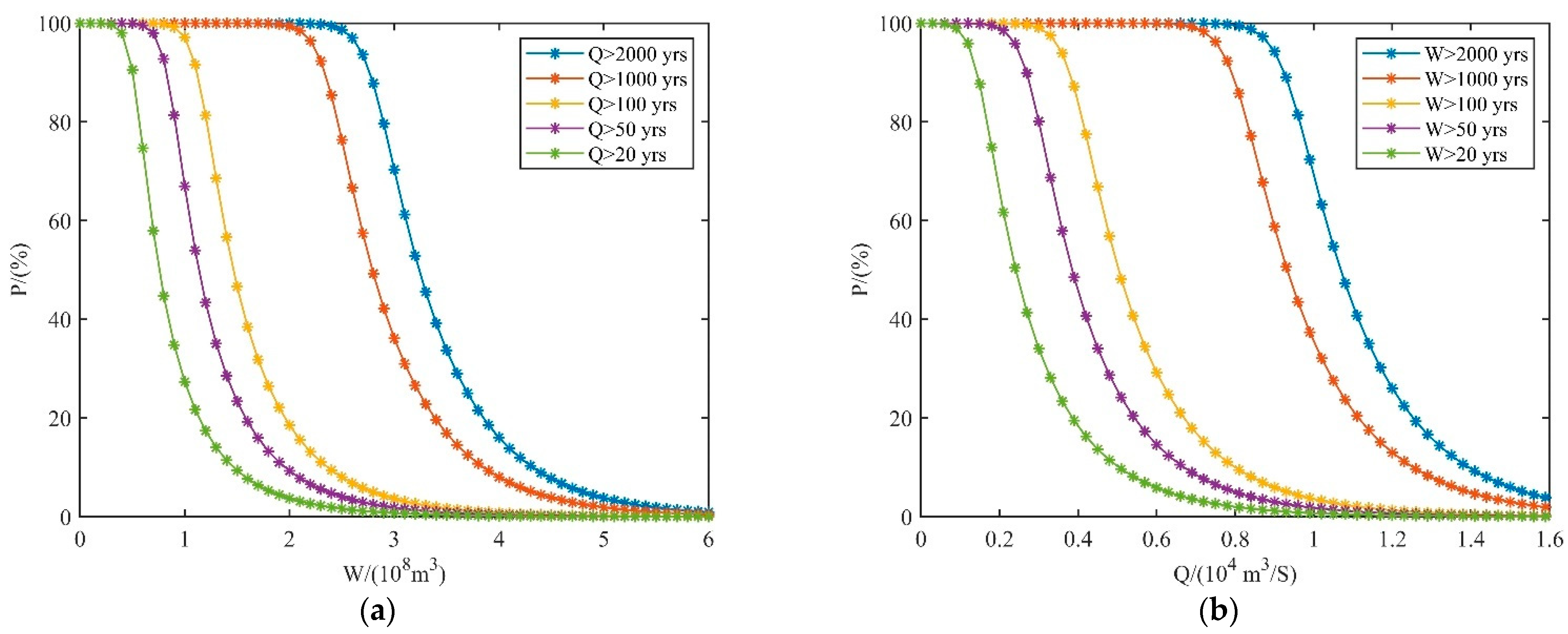
4.4. Estimating Joint and Condtional Probabilities

The estimation of joint and conditional probabilities for extreme flood events plays a vital role in reservoir flood control operation management. Simultaneous consideration of the probability of flood peak and flood volume exceeding a certain threshold can be invaluable. The joint exceedance probability is the reciprocal value of the joint OR return period. Thus, for the extraordinary flood event in 1963, the joint OR probability of both the flood peak exceeding 4250 m³/s and 1-day AMFV exceeding 1.6 × 10⁸ m³ is approximately 0.77%.

Considering reservoir flood control, the flood frequency analysis not only focuses on considering the joint probabilities of Q-V pairs exceeding a certain threshold, but also aims to estimate the conditional probabilities of extreme flood events. The outcomes of conditional probabilities are shown in Figure 8. The conditional probability curves of 1-day AMFV when AMFP exceeds a certain threshold are exhibited in Figure 8a. We focus exemplarily on the AMFP exceeding the design flood values with a 100-year (design standard) return period. The conditional probabilities of 1-day AMFV with 100-year and 2000-year return periods are 88% and 5.02%, respectively. The conditional probability results of 1-day AMFV with different return periods when the AMFP exceeds the design flood values with 100-year (design standard) and 2000-year (check standard) return periods, respectively, are summarized in

Table 7. The conditional probabilities of 1-day AMFV when the AMFP exceeds the design flood values with 100-year and 2000-year return periods.

Return Period (Year)		2000	1000	100	50	20
Design flood Wp (108 m3)		2.79	2.36	1.14	0.84	0.51
Conditional probability (%)	100-year AMFP	5.02	10.05	88.00	99.63	99.99
	2000-year AMFP	88.51	99.60	99.99	99.99	99.99

. The results indicate that, with the high correlation between AMFP and 1-day AMFV, the probability of large flood volume values with the same return period would be high if an extraordinary flood peak occurred.

5. Conclusions

This study aimed to investigate the influence of non-stationarity on flood characteristics, considering the dependence between flood peak and flood volume under a changing underlying surface, using nonstationary univariate and bivariate flood frequency analysis models in the Longmen Reservoir in North China. The following main conclusions can be drawn from this study.

(1)

The 1-day AMFV exhibits the highest significant correlation with AMFP, which demonstrates the desirability and indispensability of bivariate flood frequency analysis. In addition, the underlying surface changes in the Longmen Reservoir contribute to the heterogeneity of flood generation identified by the statistical methods and physical basis analysis. A significant change point is detected in the year 1979 for 1-day AMFV, but the AMFP is shown to be homogenous.

(2)

From univariate nonstationary flood frequency analysis of 1-day AMFV, the fitting performance of mixture distribution is superior to the traditional stationary P-III distribution. Due to the increase of forest land area and some hydraulic engineering construction, the design floods of 1-day AMFV with different return periods estimated by MD are generally smaller than the ones estimated by P-III distribution.

(3)

In the case of bivariate analysis, copula-based joint distribution was developed and performed using the stationary P-III distribution for AMFP and nonstationary MD for 1-day AMFV as marginal distributions. There is a relatively large increase for the design floods estimated by bivariate nonstationary joint distribution compared with the ones estimated in a univariate nonstationary context, which can be concluded and proved by rigorous mathematical formula derivation. Furthermore, the results of joint and conditional probabilities demonstrate that, assuming the flood peak and volume share the same return period, the conditional probability of 1-day AMFV exceeding the threshold is likely to be high when the AMFP exceeds the design flood associated with the return period.

References

1. Meaurio, M.; Zabaleta, A.; Boithias, L.; Epelde, A.M.; Sauvage, S.; Sánchez-Pérez, J.-M.; Srinivasan, R.; Antiguedad, I. Assessing the hydrological response from an ensemble of CMIP5 climate projections in the transition zone of the Atlantic region (Bay of Biscay). J. Hydrol. 2017, 548, 46–62. [Google Scholar] [CrossRef]
2. Tofiq, F.A.; Guven, A. Prediction of design flood discharge by statistical downscaling and General Circulation Models. J. Hydrol. 2014, 517, 1145–1153. [Google Scholar] [CrossRef]
3. Tofiq, F.A.; Güven, A. Potential changes in inflow design flood under future climate projections for Darbandikhan Dam. J. Hydrol. 2015, 528, 45–51. [Google Scholar] [CrossRef]
4. Huziy, O.; Sushama, L.; Khaliq, M.N.; Laprise, R.; Lehner, B.; Roy, R. Analysis of streamflow characteristics over Northeastern Canada in a changing climate. Clim. Dyn. 2013, 40, 1879–1901. [Google Scholar] [CrossRef] [Green Version]
5. Yin, J.; Guo, S.; He, S.; Guo, J.; Hong, X.; Liu, Z. A copula-based analysis of projected climate changes to bivariate flood quantiles. J. Hydrol. 2018, 566, 23–42. [Google Scholar] [CrossRef]
6. Yin, J.; Guo, S.; Liu, Z.; Yang, G.; Zhong, Y.; Liu, D. Uncertainty Analysis of Bivariate Design Flood Estimation and its Impacts on Reservoir Routing. Water Resour. Manag. 2018, 32, 1795–1809. [Google Scholar] [CrossRef]
7. Guo, A.J.; Chang, J.X.; Wang, Y.M.; Huang, Q.; Li, Y.Y. Uncertainty quantification and propagation in bivariate design flood estimation using a Bayesian information-theoretic approach. J. Hydrol. 2020, 584, 124677. [Google Scholar] [CrossRef]
8. Das, J.; Jha, S.; Goyal, M.K. Non-stationary and copula-based approach to assess the drought characteristics encompassing climate indices over the Himalayan states in India. J. Hydrol. 2019, 580, 124356. [Google Scholar] [CrossRef]
9. Jha, S.; Das, J.; Goyal, M.K. Low frequency global-scale modes and its influence on rainfall extremes over India: Nonstationary and uncertainty analysis. Int. J. Clim. 2020, 41, 1873–1888. [Google Scholar] [CrossRef]
10. Huang, K.; Chen, L.; Zhou, J.; Zhang, J.; Singh, V.P. Flood hydrograph coincidence analysis for mainstream and its tributaries. J. Hydrol. 2018, 565, 341–353. [Google Scholar] [CrossRef]
11. Requena, A.I.; Mediero, L.; Garrote, L. A bivariate return period based on copulas for hydrologic dam design: Accounting for reservoir routing in risk estimation. Hydrol. Earth Syst. Sci. 2013, 17, 3023–3038. [Google Scholar] [CrossRef] [Green Version]
12. Salvadori, G.; De Michele, C. Multivariate multiparameter extreme value models and return periods: A copula approach. Water Resour. Res. 2010, 46, 219–233. [Google Scholar] [CrossRef]
13. Zhang, L.; Singh, V.P. Bivariate Flood Frequency Analysis Using the Copula Method. J. Hydrol. Eng. 2006, 11, 150–164. [Google Scholar] [CrossRef]
14. Zhang, X.; Duan, K.; Dong, Q. Comparison of nonstationary models in analyzing bivariate flood frequency at the Three Gorges Dam. J. Hydrol. 2019, 579, 124208. [Google Scholar] [CrossRef]
15. Hu, Y.; Liang, Z.; Huang, Y.; Yao, Y.; Wang, J.; Li, B. A nonstationary bivariate design flood estimation approach coupled with the most likely and expectation combination strategies. J. Hydrol. 2021, 605, 127325. [Google Scholar] [CrossRef]
16. Brunner, M.I.; Sikorska, A.E.; Seibert, J. Bivariate analysis of floods in climate impact assessments. Sci. Total Environ. 2017, 616–617, 1392–1403. [Google Scholar] [CrossRef]
17. Duan, K.; Mei, Y.; Zhang, L. Copula-based bivariate flood frequency analysis in a changing climate—A case study in the Huai River Basin, China. J. Earth Sci. 2016, 27, 37–46. [Google Scholar] [CrossRef]
18. Parent, E.; Favre, A.-C.; Bernier, J.; Perreault, L. Copula models for frequency analysis what can be learned from a Bayesian perspective? Adv. Water Resour. 2014, 63, 91–103. [Google Scholar] [CrossRef]
19. Villarini, G. On the seasonality of flooding across the continental United States. Adv. Water Resour. 2016, 87, 80–91. [Google Scholar] [CrossRef] [Green Version]
20. Yan, L.; Xiong, L.; Liu, D.; Hu, T.; Xu, C.-Y. Frequency analysis of nonstationary annual maximum flood series using the time-varying two-component mixture distributions. Hydrol. Process. 2016, 31, 69–89. [Google Scholar] [CrossRef]
21. Alila, Y.; Mtiraoui, A. Implications of heterogeneous flood-frequency distributions on traditional stream-discharge prediction techniques. Hydrol. Process. 2002, 16, 1065–1084. [Google Scholar] [CrossRef]
22. Villarini, G.; Smith, J.A. Flood peak distributions for the eastern United States. Water Resour. Res. 2010, 46, W06504. [Google Scholar] [CrossRef] [Green Version]
23. Zeng, H.; Feng, P.; Li, X. Reservoir Flood Routing Considering the Non-Stationarity of Flood Series in North China. Water Resour. Manag. 2014, 28, 4273–4287. [Google Scholar] [CrossRef]
24. Ping, F.; Xin, L. Bivariate frequency analysis of non-stationary flood timeseries based on Copula methods. J. Hydraul. Eng. 2013, 44, 1137–1147, (In Chinese with English abstract). [Google Scholar] [CrossRef]
25. Li, J.; Zheng, Y.; Wang, Y.; Zhang, T.; Feng, P.; Engel, B.A. Improved Mixed Distribution Model Considering Historical Extraordinary Floods under Changing Environment. Water 2018, 10, 1016. [Google Scholar] [CrossRef] [Green Version]
26. Yan, L.; Xiong, L.; Ruan, G.; Xu, C.-Y.; Yan, P.; Liu, P. Reducing uncertainty of designfloods of two-component mixture distributions by utilizing flood timescale to classify flood types in seasonally snow covered region. J. Hydrol. 2019, 574, 588–608. [Google Scholar] [CrossRef]
27. Jiang, C.; Xiong, L.; Xu, C.-Y.; Guo, S. Bivariate frequency analysis of nonstationary low-flow series based on the time-varying copula. Hydrol. Process. 2014, 29, 1521–1534. [Google Scholar] [CrossRef]
28. Wen, T.; Jiang, C.; Xu, X. Nonstationary Analysis for Bivariate Distribution of Flood Variables in the Ganjiang River Using Time-Varying Copula. Water 2019, 11, 746. [Google Scholar] [CrossRef] [Green Version]
29. Xie, P.; Chen, G.; Lei, H. Hydrological alteration analysis method based on Hurst coefficient. J. Basic Sci. Eng. 2009, 17, 32–39. (In Chinese) [Google Scholar]
30. Hurst, H.E.; Black, R.P.; Simaika, Y.M. Long-Term Storage: An Experimental Study. J. R. Stat. Soc. Ser. A (Gen.) 1966, 129, 591–593. [Google Scholar] [CrossRef]
31. Bărbulescu, A.; Serban, C.; Mafteiv, C. Statistical analysis and evaluation of Hurst coefficient for annual and monthly precipitation time series. WSEAS Trans. Math. 2010, 9, 791–800. [Google Scholar] [CrossRef]
32. Pettitt, A.N. A Non-Parametric Approach to the Change-Point Problem. J. R. Stat. Soc. Ser. C (Appl. Stat.) 1979, 28, 126–135. [Google Scholar] [CrossRef]
33. Brown, M.B.; Forsythe, A.B. Robust Tests for the Equality of Variances. J. Am. Stat. Assoc. 1974, 69, 364–367. [Google Scholar] [CrossRef]
34. Fraedrich, K.; Jiang, J.; Gerstengarbe, F.-W.; Werner, P.C. Multiscale detection of abrupt climate changes: Application to River Nile flood levels. Int. J. Climatol. 1997, 17, 1301–1315. [Google Scholar] [CrossRef]
35. Salvadori, N. Evaluation of Non-Stationarity in Annual Maximum Flood Series of Moderately Impaired Watersheds in the Upper Midwest and Northeastern United States. Master’s Thesis, Michigan Technological University, Houghton, MI, USA, 2013. [Google Scholar]
36. Singh, K.P.; Sinclair, R.A. Two-Distribution Method for Flood Frequency Analysis. J. Hydraul. Div. 1972, 98, 29–44. [Google Scholar] [CrossRef]
37. Evin, G.; Merleau, J.; Perreault, L. Two-component mixtures of normal, gamma, and Gumbel distributions for hydrological applications. Water Resour. Res. 2011, 47, W08525. [Google Scholar] [CrossRef]
38. Villarini, G.; Smith, J.A.; Baeck, M.L.; Krajewski, W.F. Examining Flood Frequency Distributions in the Midwest U.S. JAWRA J. Am. Water Resour. Assoc. 2011, 47, 447–463. [Google Scholar] [CrossRef]
39. Grego, J.M.; Yates, P.A. Point and standard error estimation for quantiles of mixed flood distributions. J. Hydrol. 2010, 391, 289–301. [Google Scholar] [CrossRef]
40. Sklar, A. Fonctions de répartition à n dimensions et leurs marges. Publ. del’Institut Statistique L’Université Paris 1959, 8, 229–231. [Google Scholar]
41. Nelsen, R.B. An Introduction to Copulas; Springer: New York, NY, USA, 1999. [Google Scholar]
42. Nelsen, R.B. An Introduction to Copulas, 2nd ed.; Springer: New York, NY, USA, 2006. [Google Scholar]
43. Shiau, J.-T.; Feng, S.; Nadarajah, S. Assessment of hydrological droughts for the Yellow River, China, using copulas. Hydrol. Process. 2007, 21, 2157–2163. [Google Scholar] [CrossRef]
44. Durante, F.; Sempi, C. Principles of Copula Theory; Chapman and Hall/CRC: Boca Raton, FL, USA, 2015. [Google Scholar] [CrossRef]
45. Salvadori, G.; De Michele, C.; Kottegoda, N.T.; Rosso, R. Extremes in Nature: An Approach Using Copulas; Water Science and Technology Library; Springer: Berlin, Germany, 2007. [Google Scholar] [CrossRef]
46. Qi, W.; Liu, J. A non-stationary cost-benefit based bivariate extreme flood estimation approach. J. Hydrol. 2018, 557, 589–599. [Google Scholar] [CrossRef]
47. Poulin, A.; Huard, D.; Favre, A.-C.; Pugin, S. Importance of Tail Dependence in Bivariate Frequency Analysis. J. Hydrol. Eng. 2007, 12, 394–403. [Google Scholar] [CrossRef] [Green Version]
48. Latif, S.; Mustafa, F. Bivariate joint distribution analysis of the flood characteristics under semiparametric copula distribution framework for the Kelantan River basin in Malaysia. J. Ocean Eng. Sci. 2020, 6, 128–145. [Google Scholar] [CrossRef]
49. Lilliefors, H.W. On the Kolmogorov-Smirnov Test for Normality with Mean and Variance Unknown. J. Am. Stat. Assoc. 1967, 62, 399–402. [Google Scholar] [CrossRef]
50. Salvadori, G.; De Michele, C. Frequency analysis via copulas: Theoretical aspects and applications to hydrological events. Water Resour. Res. 2004, 40, W12511. [Google Scholar] [CrossRef]
51. Shiau, J.T. Return period of bivariate distributed extreme hydrological events. Stoch. Environ. Res. Risk Assess. 2003, 17, 42–57. [Google Scholar] [CrossRef]
52. Xiao, Y.; Guo, S.L.; Liu, P.; Fang, B. Derivation of design flood hydrograph based on Copula function. Eng. J. Wuhan Univ. 2007, 4, 13–17, (In Chinese with English abstract). [Google Scholar]
53. Hosking, J.R.M. L-Moments: Analysis and Estimation of Distributions Using Linear Combinations of Order Statistics. J. R. Stat. Soc. Ser. B Stat. Methodol. 1990, 52, 105–124. [Google Scholar] [CrossRef]
Figure 1. Schematic diagram of the Longmen Reservoir catchment and its location in the Daqing River Basin.
Water 14 00604 g001
Figure 2. The land use and land cover of the Longmen Reservoir in the years (a) 1970, (b) 1980, and (c) 2000; (d)The area percentages of land use types in three years.
Water 14 00604 g002
Figure 3. The fitting curves of MD and P-III distribution for 1-day AMFV.
Water 14 00604 g003
Figure 4. (a) Fitting performance and (b) PP-plot between theoretical and empirical joint distributions.
Water 14 00604 g004
Figure 5. The 3D plots of the AMFP and 1-day AMFV pair for (a) copula function joint distribution, (b) OR-RP, (c) AND-RP.
Water 14 00604 g005
Figure 6. The isolines of flood peak-volume pairs under joint (a) OR-RP and (b) AND-RP conditions, respectively.
Water 14 00604 g006
Figure 7. The isolines of (a) OR-RP and (b) AND-RP, respectively, for different univariate return periods of AMFP and 1-day AMFV pairs.
Water 14 00604 g007
Figure 8. The conditional probability curves of (a) 1-day AMFV and (b) AMFP.
Water 14 00604 g008