A Stacking Ensemble Learning Model for Monthly Rainfall Prediction in the Taihu Basin, China

Abstract

The prediction of monthly rainfall is greatly beneficial for water resources management and flood control projects. Machine learning (ML) techniques, as an increasingly popular approach, have been applied in diverse climatic regions, showing their respective superiority. On top of that, the ensemble learning model that synthesizes the advantages of different ML models deserves more attention. In this study, an ensemble learning model based on stacking approach was proposed. Four prevalent ML models, namely k-nearest neighbors (KNN), extreme gradient boosting (XGB), support vector regression (SVR), and artificial neural networks (ANN) are taken as base models. To combine the outputs from the base models, the weighting algorithm is used as second-layer learner to generate predictions. Large-scale climate indices, large-scale atmospheric variables, and local meteorological variables were used as predictors. R², RMSE and MAE, were used as evaluation metrics. The results show that the performance of base models varied among the nine stations in the Taihu Basin, while the stacking approach generally performed better than the four base models. The stacking model showed better performance in spring and winter than in summer and autumn. During wet months, the accuracy of model prediction varied more significantly. On the whole, based on performance evaluation measures, it is concluded that the proposed stacking ensemble multi-ML model can provide a flexible and reasonable prediction framework applicable to other regions.

1. Introduction

Rainfall is an essential component in the hydrological cycle. Rainfall prediction is a fundamental issue in hydrological application. Reliable rainfall prediction is principal for water resource management, agriculture and flood control projects [1,2,3]. In the current context of climate change [4] and intense human activity, rainfall pattern becomes more complicated; thus, rainfall prediction remains a significant and demanding problem [5,6].

Generally, for modeling precipitation, numerical models based on the physical mechanisms and the statistical models were commonly employed [7,8]. The numerical models are based on the physical equations, including the complex process of atmosphere, ocean and land [9,10]. A large amount of data, such as temperature, pressure and moisture are acquired to drive the numerical models, which expends a lot of calculation costs. The statistical model is an approach of acquiring the features of historical rainfall time series and then predicting the evolution based on these features. The autoregressive model (AR) [11], the autoregressive moving average (ARMA) model [12,13] and the autoregressive moving integrated average (ARIMA) model [14,15] have been widely used for hydrological series predicting.

Machine learning (ML) techniques, as an increasingly popular approach, provide an attractive alternative to traditional methods for rainfall prediction [16], driven by flexible predictor datasets [17,18]. It can take advantage of all kinds of information, including, but not limited to, atmospheric, geographical and oceanic factors to predict the target [19,20]. Multiple machine learning methods have been employed for predicting rainfall. Yu et al. [21] compared the effectiveness of support vector regression (SVR) and random forest (RF) in radar-derived rainfall forecasting in three reservoir catchments in Taiwan and found that SVR was more accurate in the estimation of rainfall. Cramer et al. [22] compared to the application of ML techniques in 20 cities around Europe and 22 cities in the United States, and found that ANN, SVR, and genetic programming (GP) showed better agreement than Markov chain, radial basis neural networks (RBNN), M5 rules, M5 model trees and K-nearest neighbors (KNN). Pour et al. [23] predicted seasonal rainfall extremes in Malaysia, and found that Bayesian artificial neural networks (BANN) performed the best, followed by SVR and RF. Sachindra et al. [24] compared the effectiveness of relevance vector machine (RVM) with ANN, SVR, and GP for downscaling reanalysis data to monthly rainfall in Australia. This research shows that RVM is recommended over GP, ANN or SVR in developing downscaling models. Diez-Sierra and del Jesus [19] predicted long tern term daily rainfall, showing that neural networks (NN) presented significantly better results when predicting the intensity of rainfall, followed by SVM, KNN and RF, with slightly worse values of R and RMSE than NN in Spain. Zeynoddin et al. [3] demonstrated that a hybrid model by integrating a linear model and non-linear ELM model was powerful for monthly rainfall prediction in a tropical region. Zhou et al. [25] compared RF, gradient boosting regression (GBM), SVR, ANN and dual-stage attention-based recurrent neural network (DA-RNN) in predicting monthly rainfall in Yangtze River Delta, China, showing that RF performed better in terms of MAE, and that RF and ANN proved to be favorable in terms of R², RMSE.

Previous studies have generally investigated an individual ML method with single structure, demonstrating their respective superiority. Considering that rainfall is affected by different factors, as well as that it shows different statistical characteristics, the individual ML model with a specific structure possesses limited ability to present the complex relationship between rainfall and diverse predictors in varying climatic regions. In recent years, ensemble learning methods, which can combine multiple ML models, have shown their advantages [26]. The stacking ensemble model is a popular one among them [27,28,29]. ‘Stacking’ is a specific type of ensemble learning which can take advantage of different base model structures to generate theoretically more promising prediction [30]. Zounemat et al. [31] summarized research on the application of ensemble learning approaches in a hydrological field, and claimed that using ensemble strategies is superior over individual machine learning models. Li et al. [32] integrated SVR, RF, elastic net regression (ENR) and extreme gradient boosting (XGB), through the stacking ensemble approach for mid-term streamflow forecasting. It was found that the application of the stacking strategy improved the ability of individual models. Wang et al. [33] compared stacking model with individual models for beach water quality prediction, finding the stacking model is the most robust one for 3 beaches in 5-year prediction. Nevertheless, the potential of stacking ensemble model in rainfall prediction has less explored.

The main objective of this study is to develop a stacking ensemble model for monthly rainfall prediction with multiple predictors and to examine the performance of the model. Specially, four machine learning models (KNN, XGB, SVR, ANN) were utilized as base learners due to their high popularity and good performance on previous studies. By means of assigning weights, the four base learners were combined to the stacking ensemble model. The performance of the stacking ensemble model is assessed by evaluation metrics R², RMSE, MAE. The predicted results are examined on an annual aggregated scale, seasonal scale, dry/intermediate/wet month months and months of extreme rainfall.

The rest of this paper is organized as follows: Section 2 introduces the study area and data. Section 3 presents a brief introduction of four machine learning models, the stacking ensemble framework, hyper-parameter optimization, evaluation metrics and categorization of dry/intermediate/wet months. Section 4 presents the results and discussions, including the comparison of model performances, the examination of the performance at different time scales, and the discussion of prediction results. Section 5 presents a summary and conclusions.

2. Study Area and Data

The Taihu basin (ranging from latitude 30°28′ N to 32°15′ N and longitude 119°11′ E to 121°53′ E) is located in the Yangtze River Delta, on the southeast coast of China, as shown in Figure 1. The total area of the watershed is approximately 36,895 km², comprising of parts of Jiangsu Province, Zhejiang Province and Anhui Province and Shanghai City. Around 80% of the Taihu basin is plain, and the remaining 20% is occupied by low hills in the western part of the Taihu basin [34], with rivers and lakes accounting for 17% of the total area of the basin [35]. The Taihu basin is located in a subtropical monsoon zone, with the average annual precipitation is 1218.1 mm [36]. Cyclonic storms and convectional rainfall frequently occurring in flood season (May to September), are the main triggers for flood events that, consequently, affect infrastructure and human lives.

For the monthly rainfall prediction, nine stations located in the Taihu Basin and its surroundings were selected, as shown in Figure 1. Since the long-term rainfall series data in the Taihu basin for access are limited, three stations (Nanjing, Nantong and Ningguo) within about 30 km from the Taihu basin were used in this study. The monthly rainfall at these adjacent stations are also subject to the similar climatic condition [37,38]. The monthly rainfall datasets for the period 1961–2019 were obtained from the China Meteorological Data Service Centre, China Meteorological Administration (CMA) (http://data.cma.cn/data/cdcdetail/dataCode/SURF_CLI_CHN_MUL_DAY_V3.0.html (accessed on 27 February 2021)).

Table 1. The geographic details and climatic characteristics of the nine stations in the study.

No.	Station	Abbr.	Longitude (°E)	Latitude (°N)	Altitude (m)	Monthly Precipitation
						Mean (mm)	Maximum (mm)	Coefficient of Variation (Cv)
1	Xujiahui	XJH	121.43	31.20	4.6	101.3	725.5	0.809
2	Baoshan	BS	121.45	31.40	5.5	94.5	570.9	0.834
3	Dongshan	DS	120.43	31.07	17.5	95.8	696.6	0.764
4	Liyang	LY	119.48	31.43	7.7	97.3	521.3	0.820
5	Pinghu	PH	121.08	30.62	5.4	103.4	569.3	0.788
6	Hangzhou	HZ	120.17	30.23	41.7	119.2	611.0	0.712
7	Nanjing	NJ	118.90	31.93	35.2	90.5	661.5	0.952
8	Nantong	NT	120.98	32.08	4.8	91.6	604.4	0.909
9	Ningguo	NG	118.98	30.62	87.3	120.8	783.2	0.730

provides the geographic details and climatic properties of the nine stations.

A total of 14 variables, including large-scale climate indices, large-scale atmospheric variables, and local meteorological variables, were used as predictors (

Table 2. Summary of candidate predictors for the stacking model.

No.	Multiscale Predictors		Data Source
1	Large-scale climate indices	Nino 3.4 index (Nino 3.4)	Hadley Centre Global Sea Ice and Sea Surface Temperature (Had-ISST). (https://psl.noaa.gov/gcos_wgsp/Timeseries/Data/nino34.long.data (accessed on 17 March 2021))
2		Southern Oscillation Index (SOI)	Climatic Research Unit, University of East Anglia. (https://crudata.uea.ac.uk/cru/data/soi/ (accessed on 8 March 2021))
3		Southern Hemisphere annular mode index (SAMI)	(http://ljp.gcess.cn/dct/page/65609 (accessed on 15 June 2021))
4		Western Pacific subtropic high intensity (WPSH)	National Climate Center (https://cmdp.ncc-cma.net/Monitoring/ (accessed on 3 June 2021))
5	Large-scale atmospheric variables	sea level pressure (15° S to 25° S, 55° E to 70° E) (SLP)	Reanalysis data of NCEP/NOAA [46] (http://www.esrl.noaa.gov/psd/cgi-bin/data/timeseries/timeseries1.pl (accessed on 17 June 2021))
6		meridional wind (20° N to 47.5° N, 105° E to 125° E) (V-wind(1))
7		meridional wind (32.5° N, 120° E) (V-wind(2))
8	Local meteorological variables	Monthly mean air temperature (°C) (Tmean)	China Meteorological Data Service Centre, China Meteorological Administration (CMA) (http://data.cma.cn/data/cdcdetail/dataCode/SURF_CLI_CHN_MUL_DAY_V3.0.html (accessed on 27 February 2021))
9		Monthly maximum air temperature (°C) (Tmax)
10		Monthly minimum air temperature (°C) (Tmin)
11		Monthly mean air pressure (Pmean)
12		Monthly mean vapor pressure (emean)
13		Relative humidity (dmean)
14		Sunshine duration (Dsun)

).

The large-scale climate indices in the prediction were the Nino 3.4 index (Nino 3.4), the southern oscillation index (SOI), the Western Pacific subtropic high intensity (WPSH) and the Southern Hemisphere annular mode Index (SAMI). Nino 3.4 is identified as the average sea surface temperatures (SST) anomaly in the region of 5° N–5° S and 170° W–120° W. The southern oscillation index (SOI) is typically calculated using the Troup’s method using the values of pressure differences from Tahiti and Darwin. Nino 3.4 and SOI are el nino southern oscillation (ENSO) indictors, which is one of the most important global atmospheric phenomena, influencing rainfall and temperature across the globe. The Western Pacific subtropic high intensity (WPSH) is measured by the geopotential height at 500 hPa in the region of 110° E–180° E and 10° N to the north [39]. The Southern Hemisphere annular mode index (SAMI) is defined as the difference in the normalized monthly zonal-mean sea level pressure between 40° S and 65° S [40]. Previous studies [39,40,41,42] demonstrated that WPSH and SAMI significantly impact the summer rainfall in the lower Yangtze River basin. The climate indices with the lag month (up to 6 months lagged) of the highest correlation coefficient were utilized as predictors, as shown in Figure S1.

The large-scale atmospheric variables used in this study were sea level pressure (SLP) and meridional wind at 850 mb (V-wind), representing large-scale circulation anomalies [43]. The sea level pressure (SLP) in the Indian Ocean is relevant to rainfall in the study region [42]. The meridional wind at 850 mb (V-wind) is commonly used as the large-scale atmospheric predictor for rainfall in varying regions [5,43,44,45]. Correlation coefficient between the large-scale atmospheric variables and rainfall was used to select the spatial grid and the lag month of the large-scale atmospheric variables. As shown in Figure 2, the spatial grids of SLP were selected by the interactive correlation analysis provided by the Physical Sciences Division in the Earth System Research Laboratory (ESRL 2008) (https://psl.noaa.gov/data/correlation/ (accessed on 7 December 2021)), and the correlation coefficient between the selected SLP with 4 months lagged and rainfall was −0.464. All the selected large-scale atmospheric variables were highly correlated with rainfall in the study region of over 0.001 statistical significance level.

The local meteorological predictors for each station were monthly maximum temperature (T_max), monthly minimum temperature (T_min), monthly mean temperature (T_mean), monthly mean pressure (P_mean), monthly mean water pressure (e_mean), monthly mean relative humidity (d_mean) and monthly sunshine duration (D_sun). These predictors were selected for representing local scale characteristics.

3. Methodology

The models are trained and evaluated using above predictors. Since regional rainfall is related to multiscale climatic and meteorological features, the 14 predictors utilized represent the factors with multiple scales associated with rainfall in the study region. In addition, rainfall data from 9 rain stations are employed, keeping nearly 90% of each station for fitting the models (training), and the remaining roughly 10% for evaluating their prediction skill (testing) [47,48]. A fifty-nine years-long time series for each station are split in two sets (shown in Figure 3): the training set for the period of 1961–2012, containing 52 years of data and the testing set for the period of 2013–2019, containing the remaining 7-year data. Predictive performance is evaluated over the testing set, which is not learned in any methods.

3.1. Machine Learning Methods

3.1.1. K-Nearest Neighbors (KNN)

K-nearest neighbors (KNN) was proposed by Cover T.M. and Hart P.E. [49]. K-nearest neighbors (KNN) is a non-linear method whose predictions are computed through the weighted mode (classification) or the weighted mean (regression) of the k nearest points to the one being predicted. The Euclidean distance metric and Manhattan distance metric are commonly used metrics for finding the closest k neighbors in the training set. Then, the predicted target is obtained by averaging these neighbors, or the weighted average according to the distance. More details on the KNN algorithm can be found in [50].

3.1.2. Extreme Gradient Boosting (XGB)

Extreme gradient boosting (XGB, also known as XGBoost) proposed by Chen and Guestrin [51], is a new application of gradient boosting machines. As the gradient boosting machines, XGB is developed through an additive training strategy. The predictions are made from weak learners that continuously develop over the mistakes from the former learners. The difference is that the gradient boosting algorithm is a negative gradient that learns a weak learner to approximate the loss function. XGB first finds the second-order Taylor approximation of the loss function at that point, and then minimizes the approximation loss function to train the weak learner. XGB can process sparse data automatically, and it is generally more than ten times faster than the conventional gradient boosting technique. For more information, readers are referred to [52].

3.1.3. Support Vector Regression (SVR)

Support vector regression (SVR) is a kind of support vector machine (SVM) [53] for performing the regression task. The general concept of SVR is that it nonlinearly maps the feature data into the high-dimensional feature space. The objective of SVR is to find a hyperplane that maximizes the margins by separating samples belonging to different groups. The data points that support the margin at a close distance from the hyperplane are known as support vectors. In SVR, mapping the feature set into the high-dimensional feature space is achieved by the kernel function. The detailed description on various kernels can be found in [47]. Previous hydrological studies of SVR application demonstrated that the radial basis function kernel was found to be effective [5,20,54,55].

3.1.4. Artificial Neural Network (ANN)

Artificial neural network (ANN) is inspired by the neurological structure of the human brain [56]. A common ANN architecture used in this study is the multiple layer perceptrons (MLP). The mathematical description of the method can be found in [57]. As a brief description, MLP is a feedforward network that consists of an input layer, hidden layer(s) and an output layer. The input layer receives external data and the output one produces the final result. The hidden layers are neurons nodes between the input and out layer, providing nonlinearity. More complex problems can be solved by increasing the hidden neurons or layers used. A neuron is a computational unit that receives input from other neurons that are interconnected with weight. The ‘activation function’ that each neuron uses receives the linear combination of inputs to produce the results in non-linear transformation. In the present study, the traditional backpropagation algorithm [58] was adopted as the learning algorithm.

3.2. Stacking Ensemble Learning

The stacking ensemble learning is proposed by Wolpert [26], taking advantage of mutual complementarity among the base models to enhance generalization ability. The process occurs by, firstly, obtaining the results predicted by a set of diverse base models, and then optimally combining the outputs from the base models using a meta-learner to generate the final prediction. To prevent overfitting, the outputs from the base models are not directly learned by the meta-model. The leave-one-out cross validation method is used in this ensemble learning strategy. The validation folds are stacked as the new dataset for the meta-model to learn, which is the reason this strategy is called “stacking”. How to integrate the base models is important. Multiple linear regression ML models such as RF, can be used as a meta-model. In our study, weights were assigned to the base models to constitute the stacking model prediction. The mathematical expression can be presented as:

$$y_{\mathrm{P},\mathrm{i}}={\displaystyle \sum _{\mathrm{m}=1}^{\mathrm{M}}{\omega }_{\mathrm{m}}{f}_{\mathrm{m},\mathrm{i}}}$$

(1)

where ω_m (m = 1, 2, …, M) is the weight assigned for each base models, f_m,i represents the prediction of the model m for the ith observation.

To obtain the optimal final prediction, the set of stacking weights were estimated by minimizing the mean square linear regression. Thus, the objective function under two constraints are as follows:

$$\mathrm{\Omega }=\arg \min {\displaystyle \sum _{\mathrm{i}=1}^{\mathrm{N}}[y_{\mathrm{O},\mathrm{i}}-{\displaystyle \sum _{\mathrm{m}=1}^{\mathrm{M}}{\omega }_{\mathrm{m}}{f}_{\mathrm{m},\mathrm{i}}}{]}^2}$$

(2)

$$\begin{array}{cc}{\omega }_{\mathrm{m}}\ge 0& \mathrm{m}=1,2,\dots ,\mathrm{M}\end{array}$$

(3)

$$\begin{array}{cc}{\displaystyle \sum _{\mathrm{m}=1}^{\mathrm{M}}{\omega }_{\mathrm{m}}=1}& \mathrm{m}=1,2,\dots ,\mathrm{M}\end{array}$$

(4)

where Ω = {ω₁, ω₂,…, ω_M} is the set of weights assigned to the base models. Two constraints are: (i) weights should be larger than or equal to zero, and (ii) the sum of the weights equals to one. This leads to a quadratic minimization problem [59], and the python package ‘qpsolvers’ was used to solve it. Through calculating the weights of the base models, the stacking model was integrated to generate the final prediction. The construction of the proposed stacking model and the overall flowchart of the adopted methodology in this study is presented in Figure 4.

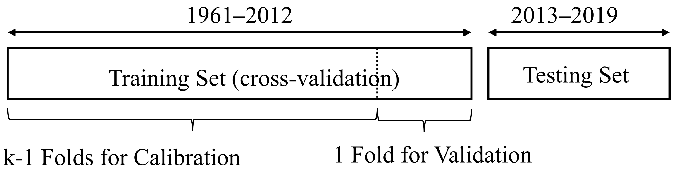
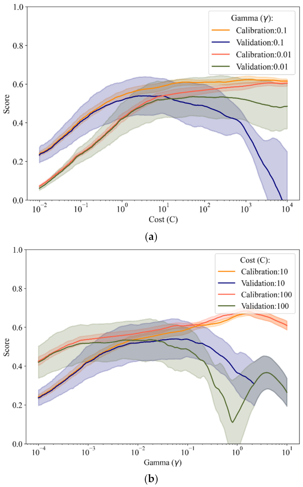
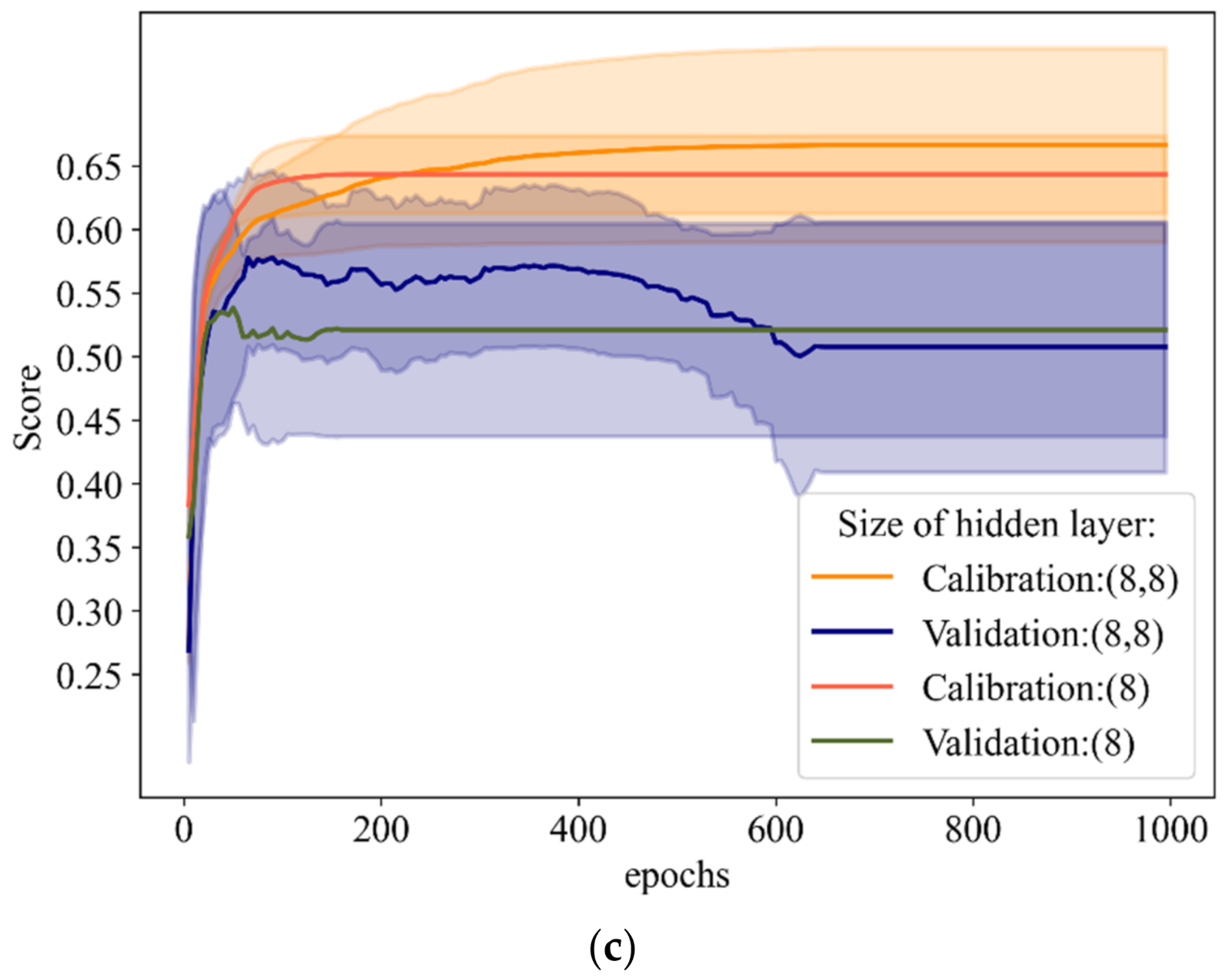
3.3. Hyper-Parameter Optimization

Hyper-parameter tuning is commonly used to construct an appropriate model for a specific prediction. The model performance varies with different selection of hyper-parameter values.

Table 3. Summary of the hyper-parameters of the four machine learning models.

Machine Learning Model	Hyper-Parameters
K-nearest neighbors (KNN)	Number of neighbors
	Weights
Extreme gradient boosting (XGB)	Number of estimators
	Learning rate
	Max depth
Support vector regression (SVR)	Cost C
	Parameter of Gaussian Kernel—Gamma(γ)
Artificial neural network (ANN)	Size of hidden layer
	Activation function
	Learning rate
	Batch size

summarizes the main hyper-parameters of the four machine learning models applied in this study. Taking SVR and ANN as examples, Figure 5 shows the process of hyper-parameter tuning of the two models. The hyper-parameters were tuned and evaluated over the training set by k-fold cross-validation [60]. K-fold cross-validation leveraging information in a small dataset helps to avoid overfitting and to produce a model that performs well on new data [61]. Figure 5a,b illustrates how the performance of SVR varies with the hyper-parameter Cost © and Gamma(γ). For SVR, the cost C and γ with the radial basis function kernel are significant hyper-parameters. It illustrates a proper value range of the cost C; γ were nearly 10⁻² to 10⁻¹ and 10 to 100, respectively. For ANN, the size of the hidden layer is an essential hyper-parameter, indicating the complexity of the learning model. In Figure 5c, ANN with a hidden layer of (8) and (8,8) were compared. Earlier convergence (nearly 190 epochs) and higher performance (R² of 0.53) over the validation set were shown on the ANN with the layer of (8) compared to one with a hidden layer of (8,8). This indicates that the relatively smaller size of hidden layer ANN has enough learning capacity, and that too large of a size of hidden layer will cause overfitting. For the machine learning model, multiple important hyper-parameters impact the model performance comprehensively; the grid search approach was utilized to optimize the combination of hyper-parameters within the specified range in this study. Then, the models with hyper-parameters tuned were applied in the testing set. There was no notable higher performance in the training set than the testing one, indicating that the models built are reasonable and capable of generalization.

3.4. Performance Evaluation

The performances of the above machine learning models were evaluated by the commonly used statistic metrics: (1) Coefficient of determination (R²), (2) root mean square error (RMSE), (3) mean absolute error (MAE). R² measures the proportion of variance explained by the model. The best possible score is 1.0; a larger value represents a better fit. RMSE evaluates the residual between observed and predicted values and is particularly sensitive to the large errors, since the errors are squared before they are averaged. the MAE is less sensitive to extreme values than the RMSE [62]. The mathematical formulas are as follows:

Coefficient of determination (R²)

$${\mathrm{R}}^2=1-\frac{{\displaystyle \sum _{\mathrm{i}=1}^{\mathrm{N}}{(y_{\mathrm{P},\mathrm{i}}-y_{\mathrm{O},\mathrm{i}})}^2}}{{\displaystyle \sum _{\mathrm{i}=1}^{\mathrm{N}}{(y_{\mathrm{O},\mathrm{i}}-{\overline{y}}_{\mathrm{O},\mathrm{i}})}^2}}$$

(5)

Root mean square error (RMSE)

$$\mathrm{RMSE}=\sqrt{\frac{1}{\mathrm{N}}{\displaystyle \sum _{\mathrm{i}=1}^{\mathrm{N}}{(y_{\mathrm{P},\mathrm{i}}-y_{\mathrm{O},\mathrm{i}})}^2}}$$

(6)

Mean absolute error (MAE)

$$\mathrm{MAE}=\frac{1}{\mathrm{N}}{\displaystyle \sum _{\mathrm{i}=1}^{\mathrm{N}}\left|y_{\mathrm{P},\mathrm{i}}-y_{\mathrm{O},\mathrm{i}}\right|}$$

(7)

where y_P,i and y_O,i are the predicted and observed monthly precipitation in test period t (test slice), respectively, i is the month of the dataset and N (= 84) is the length (number of samples in the test set) in period t (2013–2019), ${\overline{y}}_{\mathrm{O},\mathrm{i}}$ is the mean values of the series y_O,i.

3.5. Categorization of Dry, Intermediate and Wet Months in Terms of Standardized Precipitation Index (SPI)

For measuring the model performance on normal, below and above normal monthly rainfall prediction, the standardized precipitation index (SPI) proposed by McKee et al. [63] was used to designate the monthly precipitation into the dry/intermediate/wet classifications. SPI was calculated using the available program from the National Drought Mitigation Centre (https://drought.unl.edu/droughtmonitoring/SPI/SPIProgram.aspx (accessed on 29 July 2021)). The SPI calculated in this study is based on representing the historical monthly precipitation record with a gamma distribution. Positive SPI values represent wet conditions; the higher the SPI, the more unusually wet a month is. Negative SPI values represent dry conditions; the lower the SPI, the more unusually dry a month is. The detailed methodology and the computation process of SPI can be found in Angelidis et al. [64].

SPI was obtained based on the observed monthly rainfall series. The calculated SPI fall into three categories, namely, ‘dry’ (SPI < −1), ‘intermediate’ (−1 ≤ SPI ≤ 1), and ‘wet’ (SPI > 1). The performance of the models above was assessed respectively in terms of the three categories.

4. Results and Discussion

4.1. Intercomparison of Model Performances

Four base models and the stacking model are constructed at nine stations in the Taihu basin for prediction of monthly rainfall. Prediction is independent for each station. The observed and predicted monthly precipitation series of all the models at the nine stations are shown in Figure S2.

Figure 6 demonstrates the prediction skills of all the models at the nine rainfall stations. Among the four base models, the model performances vary in terms of R², RMSE, and MAE. The R² ranges from 0.29 to 0.70. The RMSE and MAE range from 48 mm to 79 mm and from 35 mm to 51 mm, respectively. It presents analogous ranges of the evaluation metrics with the previous predictions at the lower reach of the Yangtze River [25], illustrating the models in this study perform in the reasonable range. Among the base models, ANN at Xujiahui had the best prediction accuracy with the highest R² and the smallest RMSE and MAE, while the accuracy of KNN was the worst in terms of the three metrics at almost all the stations. There was no base model that performed best at all the stations.

We then compared the performance of the base models and the stacking model. The best models selected in terms of R² and RMSE were same at the nine stations (shown in Table S1), and the stacking model performed best at two stations. In terms of MAE, the stacking model performed best at four stations. This implies that, through combining ML models of diverse structures, the stacking model has the potential to over-perform all its base models. At the other stations, the stacking model showed analogous accuracy with the best base models. It should be noted that, though the stacking model was not selected as the best one at all the nine stations, the variation of each metric was lower, implying that the stacking model can produce more robust predictions at regional scale. Additionally, as shown in

Table 4. Evaluation metrics averaged over the nine stations at different time scales.

	Evaluation Metrics	KNN	XGB	SVR	ANN	Stack
All months	R2	0.407	0.526	0.523	0.532	0.526
	RMSE (mm)	68.72	61.57	61.65	60.92	61.51
	MAE (mm)	46.34	42.41	43.16	42.47	41.65
Annual aggregation scale	RMSE (%)	26.12	22.33	22.12	24.63	23.34
	MAE (%)	21.39	18.31	18.61	21.02	19.40
Spring	RMSE (mm)	43.82	45.74	45.79	47.16	44.22
	MAE (mm)	33.86	37.18	36.88	37.89	35.58
Summer	RMSE (mm)	95.50	87.56	87.06	85.19	87.44
	MAE (mm)	73.85	66.46	66.21	66.72	66.82
Autumn	RMSE (mm)	77.17	64.35	64.02	62.89	65.27
	MAE (mm)	50.55	44.21	44.03	42.61	43.15
Winter	RMSE (mm)	34.45	27.46	29.52	28.06	26.22
	MAE (mm)	27.09	21.77	25.54	22.67	21.05
Dry months	RMSE (mm)	61.05	47.56	49.45	43.03	46.78
	MAE (mm)	49.90	37.47	40.39	32.33	35.87
Intermediate months	RMSE (mm)	36.98	40.53	42.27	43.94	38.77
	MAE (mm)	28.08	32.26	33.06	33.98	30.21
Wet months	RMSE (mm)	121.23	101.22	99.03	96.82	103.43
	MAE (mm)	97.86	73.15	72.94	71.33	76.69
Months of extreme rainfall	RMSE (mm)	197.70	172.36	164.65	157.80	173.26
	MAE (mm)	188.36	162.22	153.26	143.32	163.38

, the stacking strategy reduced MAE more effectively than RMSE, since MAE evaluates the average magnitude, while RMSE is more sensitive to the large errors, which are squared before they are averaged. This indicates that, except for the magnification of the large errors generally occurring at extreme rainfall samples [65], the stacking model appeared to be more favorable in the measurement of average performance in the entire rainfall series prediction. The best model for each station selected in terms of R², RMSE and MAE is shown in Table S1.

4.2. Prediction Skills at Different Time Scales

It is also of importance to predict annual, seasonal and other scales in the water resources management. Thus, we examined the model performance at annual aggregated scale, seasonal scale, dry/intermediate/wet months and months of extreme rainfall.

At the annual aggregation scale, Table 4 shows the evaluation metrics (RMSE and MAE) of the five models at nine rainfall stations over the study region. The RMSE of the stacking model at the annual aggregation scale was 157.5–399.7 mm (accounting for 15–35% of the annual precipitation averaged over the 1961–2019 period), and MAE was 157.6–336.7 mm (accounting for 11–30%). Among the base models, SVR performed satisfactorily at the annual aggregation scale, with an RMSE of 135.7–333.8 mm (accounting for 10–31%) and MAE of 110.9–299.6 mm (accounting for 9–25%). Generally, in terms of the performance at the annual aggregation scale, the stacking model and ML models, such as SVR and XGB, showed good ability in readily applying to long-term rainfall prediction for regional water resources management.

Over four seasons, rainfall shows significantly seasonal variability in the study region. The average monthly rainfall (1961–2019) at the stations was 81.5–137.1 mm in spring (from March to May), 151.9–194.8 mm in summer (from June to August), 65.0–96.8 mm in autumn (from September to November), and 39.9–73.0 mm in winter (from December to February). Thus, evaluation metrics (RMSE and MAE), the percentage of which accounts for average monthly rainfall over four seasons, were evaluated at the seasonal scale, shown in Figure 7. In terms of RMSE and MAE, the prediction in winter was the most accurate, followed by spring and autumn. The evaluation metrics were highest in summer considering its largest amount of rainfall over four seasons. While, in terms of the percentage of RMSE and MAE, the prediction in spring was the most accurate, similar in summer and winter, but worst in autumn. Generally, the stacking model performed better in spring and winter than in summer and autumn. It is noted that previous studies [40,42,66] have highlighted the importance of accurately predicting summer rainfall. Future work is needed to explore suitable models and the main factors for summer rainfall prediction in this region.

The prediction from the above models was further compared in terms of dry/intermediate/wet months. As mentioned earlier, SPI was used as the index for classifying the categorization. The SPI was calculated based on observed monthly rainfall series, and divided all months into three categories, namely, ‘dry’ (SPI < −1), ‘intermediate’ (−1 ≤ SPI ≤ 1), and ‘wet’ (SPI > 1). The scatter plots of the stacking model are presented in Figure 8. The results of base models are shown in Figure S3. It revealed that all the models underestimated rainfall for the wet months, and slightly overestimated rainfall for the dry months.

The predictions for intermediate and dry months were within a minor error range. The prediction error on wet conditions was high, and rainfall prediction for wet JJA (June-July-August) months was the most underestimated, indicating that the wet feature is the most difficult for the machine learning models to capture. The evaluation metrics (RMSE and MAE) for dry/intermediate/wet months by the stacking model and the base models shown in Table 4 also offered the same indication. Similar results were also found in other climate regions [5,24]. Further work is needed to pay attention on wet JJA rainfall prediction, which is crucial to the regional flood prevention.

Extreme precipitation deserves special attention in the Taihu basin, considering that intensive precipitation during the ‘Plum Rain Season’ (the rainy season from late June to early July in the Yangtze Plain) and typhoon season may cause flooding [35]. We compared the prediction skill of the above models on precipitation above 300 mm, which is considered as extreme rainfall in the study region. Since the samples of extreme rainfall are a tiny part in the series (nearly 3%), the extreme rainfall is generally underestimated by the above models. Such a feature seems difficult for models to capture. The evaluation metrics on extreme rainfall are shown in Table 4. They indicated that ANN showed the greatest predictive ability, followed by SVR. The stacking model performed comparable to XGB. KNN showed poor predictive power on extreme rainfall, since the stacking model with the weight-distributed strategy is influenced by all the base models. One of the base models with poor performance may reduce the prediction ability of the stacking one. Other ML models can be utilized as an alternative in the flexible stacking framework for enhancing the predictive skill.

4.3. Discussions

Irrespective of the models used in prediction, there are quite differing prediction effects shown among the nine stations. Higher performance was shown at Xujiahui and Ningguo station, with R² of 0.642 and 0.645, respectively, while lower performance was shown at Nanjing, with R² only reaching 0.438 by the stacking model, as depicted in Figure 9. The certain possible reasons that may impact the performance are addressed as follows.

One of the crucial reasons is likely associated with different characteristics in the rainfall series among these stations. We used C_V and probability density of time series as examples to demonstrate the various features. Figure 9 shows the performance of the stacking model contrast to the coefficient of variation (C_V) at the nine stations. The higher C_V indicated a more disperse rainfall distribution, which may increase the difficulty of the series prediction. In Table S2, lower C_V are shown in all predicted series than in observational ones, which indicates that the dispersion feature in the time series is difficult to capture. Figure 10 shows the probability density distribution of observations and predictions by the stacking model at the nine stations. Lower probability density in distribution tails and excessive distribution around 100 mm also show that the predicted rainfall is prone to concentrate on moderate values, making the dispersion of the series difficult to reproduce. Further research is needed to examine the main features of time series that impact the prediction performance.

Another characteristic that may affect the prediction is the discrepancy between the rainfall distributions for the training set (1961–2012) and the testing set (2013–2019). Figure 10 shows that the probability distribution in the range of 0–100 mm significantly reduces, while the monthly rainfall larger than 200 mm occurs more frequently during the testing period (2013–2019) at most of stations. In comparison, there are similar probability distributions in the training and testing period at Xujiahui and Ningguo station, conducive to high prediction accuracy at these stations. It implies that the characteristics of training and testing sets have a notably high impact on the prediction accuracy. Further works can consider the statistical characteristics in the ML prediction model construction to enhance the predictive ability.

The division of training and testing sets is an inevitable issue in time series prediction. Generally, for building a statistical predictive model, the training set and the testing set are required to contain the same distribution [67], which is conducive to achieving good prediction results. However, due to the complexities in the change of rainfall characteristics [4] which is caused by natural and anthropogenic factors, the physical factors that impact rainfall characteristics are needed in the models as prediction factors in the long term rainfall prediction to reveal this change. In addition, other climatic and meteorological variables utilized as predictors also show non-stationarity and complexity in dynamic climate systems [68]. Identifying major drivers of regional rainfall for mapping relationship construction is also important to enhance the predictive ability.

5. Conclusions

In this study, a stacking ensemble learning model and its base models were compared for the prediction of monthly rainfall at nine stations in the Taihu basin, China, using large-scale climate indices, large-scale atmospheric variables, and local meteorological variables as predictors. Principal conclusions of the study are as follows:

(1)

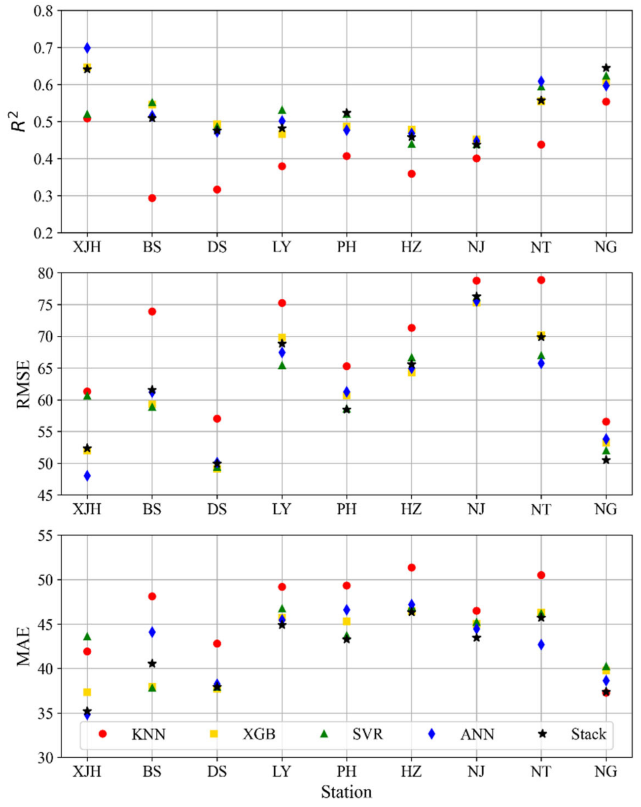
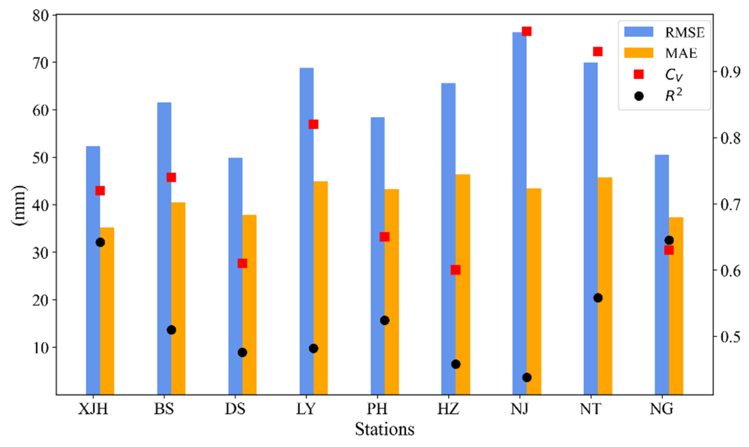
Through combining models of diverse structures, the stacking model showed the potential to over-perform all the base models. In terms of different evaluation metrics, the results varied among the models. In terms of R² and RMSE, the stacking model performed best at two stations (Pinghu and Ningguo). In terms of MAE, the stacking model performed best at four stations (Liyang, Pinghu, Hangzhou and Nanjing). At the other rainfall stations, the stacking approach also showed satisfactory performance, close to the best one of the individual base models, and especially showed favorable results in term of MAE. Thus, the proposed stacking model can produce reasonable predictions for the entire rainfall series.

(2)

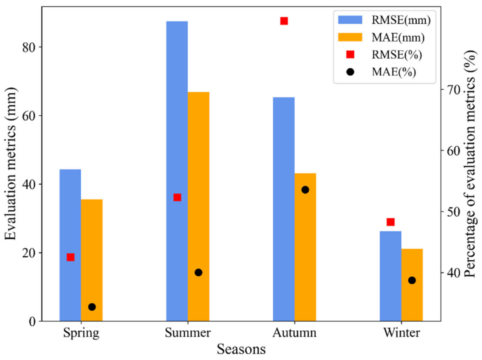
At the annual aggregation scale, the stacking model and ML models (SVR and XGB) performed satisfactorily, showing good ability in applying long-term rainfall prediction for regional water resources management. Over four seasons, the stacking model generally showed better performance in spring and winter than in summer and autumn. In terms of dry/intermediate/wet months, the models showed a greater minor error range in dry and intermediate months than wet months, with underestimation of the wet months and slight overestimation of the dry months.

(3)

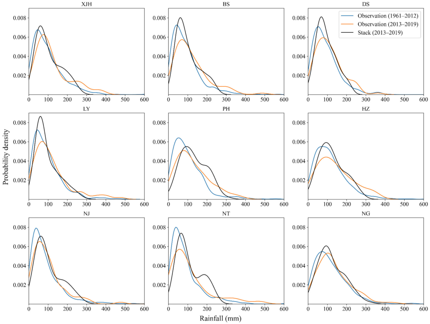
In terms of extreme rainfall, ANN outperformed the stacking model. The ML models generally undervalue extreme rainfall. ANN, relatively, generated the closest prediction, showing the potential to capture the extreme wet condition. Further work is needed to explore ML methods to enhance the ability of predicting extreme rainfall, especially in regions vulnerable to flooding.

In this study, a stacking ensemble model of combining different machine learning model structures was proposed in rainfall prediction. In this flexible stacking framework, the attempts to improve base-learners and meta-learners were promising to enhance the prediction ability in further research. In addition to the model structures, the difference between training and testing data distributions also affected the prediction performance. Further study should focus on the variability in rainfall series, the identification of important drivers to enhance the prediction ability and the examination of more ML models, such as recurrent neural network (RNN) [58], under the ensemble framework. The data-driven model with the stacking ensemble framework is readily generalized to other climatic regions, using climatic, meteorological and diverse information.

References

1. Ali, M.; Deo, R.C.; Downs, N.J.; Maraseni, T. Multi-stage hybridized online sequential extreme learning machine integrated with Markov Chain Monte Carlo copula-Bat algorithm for rainfall forecasting. Atmos. Res. 2018, 213, 450–464. [Google Scholar] [CrossRef]
2. Bagirov, A.; Mahmood, A.; Barton, A. Prediction of monthly rainfall in Victoria, Australia: Clusterwise linear regression approach. Atmos. Res. 2017, 188, 20–29. [Google Scholar] [CrossRef]
3. Zeynoddin, M.; Bonakdari, H.; Azari, A.; Ebtehaj, I.; Gharabaghi, B.; Madvar, H.R. Novel hybrid linear stochastic with non-linear extreme learning machine methods for forecasting monthly rainfall a tropical climate. J. Environ. Manag. 2018, 222, 190–206. [Google Scholar] [CrossRef] [PubMed]
4. Climate Change 2014: Synthesis Report. Contribution of Working Groups I, II and III to the Fifth Assessment Report of the Intergovernmental Panel on Climate Change. Geneva. 2014. Available online: https://www.ipcc.ch/report/ar5/syr (accessed on 20 December 2021).
5. Das, P.; Chanda, K. Bayesian Network based modeling of regional rainfall from multiple local meteorological drivers. J. Hydrol. 2020, 591, 125563. [Google Scholar] [CrossRef]
6. Abbot, J.; Marohasy, J. Input selection and optimisation for monthly rainfall forecasting in Queensland, Australia, using artificial neural networks. Atmos. Res. 2014, 138, 166–178. [Google Scholar] [CrossRef]
7. Shahrban, M.; Walker, J.; Wang, Q.; Seed, A.; Steinle, P. An evaluation of numerical weather prediction based rainfall forecasts. Hydrol. Sci. J. 2016, 61, 2704–2717. [Google Scholar] [CrossRef] [Green Version]
8. Ali, M.; Deo, R.C.; Downs, N.J.; Maraseni, T. Chapter 3—Monthly Rainfall Forecasting with Markov Chain Monte Carlo Simulations Integrated with Statistical Bivariate Copulas. In Handbook of Probabilistic Models; Samui, P., Tien Bui, D., Chakraborty, S., Deo, R.C., Eds.; Butterworth-Heinemann: Boston, MA, USA, 2020; pp. 89–105. ISBN 978-0-12-816514-0. [Google Scholar]
9. Giebel, G.; Kariniotakis, G. Wind power forecasting—A review of the state of the art. In Renewable Energy Forecasting: From Models to Applications; Woodhead Publishing: Cambridge, UK, 2017; ISBN 978-0081005040. [Google Scholar]
10. Yu, W.; Nakakita, E.; Jung, K. Flood Forecast and Early Warning with High-Resolution Ensemble Rainfall from Numerical Weather Prediction Model. Procedia Eng. 2016, 154, 498–503. [Google Scholar] [CrossRef] [Green Version]
11. Carlson, R.F.; MacCormick, A.J.A.; Watts, D.G. Application of Linear Random Models to Four Annual Streamflow Series. Water Resour. Res. 1970, 6, 1070–1078. [Google Scholar] [CrossRef]
12. Burlando, P.; Rosso, R.; Cadavid, L.G.; Salas, J.D. Forecasting of short-term rainfall using ARMA models. J. Hydrol. 1993, 144, 193–211. [Google Scholar] [CrossRef]
13. Valipour, M.; Banihabib, M.E.; Behbahani, S.M.R. Comparison of the ARMA, ARIMA, and the autoregressive artificial neural network models in forecasting the monthly inflow of Dez dam reservoir. J. Hydrol. 2012, 476, 433–441. [Google Scholar] [CrossRef]
14. Rahman, M.A.; Yunsheng, L.; Sultana, N. Analysis and prediction of rainfall trends over Bangladesh using Mann–Kendall, Spearman’s rho tests and ARIMA model. Arch. Meteorol. Geophys. Bioclimatol. Ser. B 2016, 129, 409–424. [Google Scholar] [CrossRef]
15. Lana, X.; Rodríguez-Solà, R.; Martínez, M.D.; Casas-Castillo, M.C.; Serra, C.; Kirchner, R. Autoregressive process of monthly rainfall amounts in Catalonia (NE Spain) and improvements on predictability of length and intensity of drought episodes. Int. J. Clim. 2020, 41. [Google Scholar] [CrossRef]
16. Basha, C.Z.; Bhavana, N.; Bhavya, P. Rainfall Prediction Using Machine Learning Amp; Deep Learning Techniques. In Proceedings of the 2020 International Conference on Electronics and Sustainable Communication Systems (ICESC), Coimbatore, India, 2–4 July 2020; pp. 92–97. [Google Scholar]
17. Ortiz-García, E.; Salcedo-Sanz, S.; Casanova-Mateo, C. Accurate precipitation prediction with support vector classifiers: A study including novel predictive variables and observational data. Atmos. Res. 2014, 139, 128–136. [Google Scholar] [CrossRef]
18. Grace, R.K.; Suganya, B. Machine Learning Based Rainfall Prediction. In Proceedings of the 2020 6th International Conference on Advanced Computing and Communication Systems (ICACCS), Coimbatore, India, 6–7 March 2020; pp. 227–229. [Google Scholar]
19. Diez-Sierra, J.; del Jesus, M. Long-term rainfall prediction using atmospheric synoptic patterns in semi-arid climates with statistical and machine learning methods. J. Hydrol. 2020, 586, 124789. [Google Scholar] [CrossRef]
20. Tian, D.; He, X.; Srivastava, P.; Kalin, L. A hybrid framework for forecasting monthly reservoir inflow based on machine learning techniques with dynamic climate forecasts, satellite-based data, and climate phenomenon information. Stoch. Hydrol. Hydraul. 2021, 1–23. [Google Scholar] [CrossRef]
21. Yu, P.-S.; Yang, T.-C.; Chen, S.-Y.; Kuo, C.-M.; Tseng, H.-W. Comparison of random forests and support vector machine for real-time radar-derived rainfall forecasting. J. Hydrol. 2017, 552, 92–104. [Google Scholar] [CrossRef]
22. Cramer, S.; Kampouridis, M.; Freitas, A.; Alexandridis, A.K. An extensive evaluation of seven machine learning methods for rainfall prediction in weather derivatives. Expert Syst. Appl. 2017, 85, 169–181. [Google Scholar] [CrossRef] [Green Version]
23. Pour, S.H.; Wahab, A.K.A.; Shahid, S. Physical-empirical models for prediction of seasonal rainfall extremes of Peninsular Malaysia. Atmos. Res. 2019, 233, 104720. [Google Scholar] [CrossRef]
24. Sachindra, D.; Ahmed, K.; Rashid, M.; Shahid, S.; Perera, B. Statistical downscaling of precipitation using machine learning techniques. Atmos. Res. 2018, 212, 240–258. [Google Scholar] [CrossRef]
25. Zhou, Z.; Ren, J.; He, X.; Liu, S. A comparative study of extensive machine learning models for predicting long-term monthly rainfall with an ensemble of climatic and meteorological predictors. Hydrol. Process. 2021, 35, e14424. [Google Scholar] [CrossRef]
26. Wolpert, D.H. Stacked generalization. Neural Netw. 1992, 5, 241–259. [Google Scholar] [CrossRef]
27. Rice, J.S.; Emanuel, R.E. How are streamflow responses to the El Nino Southern Oscillation affected by watershed characteristics? Water Resour. Res. 2017, 53, 4393–4406. [Google Scholar] [CrossRef]
28. Zhai, B.; Chen, J. Development of a stacked ensemble model for forecasting and analyzing daily average PM2.5 concentrations in Beijing, China. Sci. Total Environ. 2018, 635, 644–658. [Google Scholar] [CrossRef] [PubMed]
29. Sun, W.; Trevor, B. A stacking ensemble learning framework for annual river ice breakup dates. J. Hydrol. 2018, 561, 636–650. [Google Scholar] [CrossRef]
30. Breiman, L. Stacked Regressions. Mach. Learn. 1996, 24, 49–64. [Google Scholar] [CrossRef] [Green Version]
31. Zounemat-Kermani, M.; Batelaan, O.; Fadaee, M.; Hinkelmann, R. Ensemble machine learning paradigms in hydrology: A review. J. Hydrol. 2021, 598, 126266. [Google Scholar] [CrossRef]
32. Li, Y.; Liang, Z.; Hu, Y.; Li, B.; Xu, B.; Wang, D. A multi-model integration method for monthly streamflow prediction: Modified stacking ensemble strategy. J. Hydroinform. 2019, 22, 310–326. [Google Scholar] [CrossRef]
33. Wang, L.; Zhu, Z.; Sassoubre, L.; Yu, G.; Liao, C.; Hu, Q.; Wang, Y. Improving the robustness of beach water quality modeling using an ensemble machine learning approach. Sci. Total Environ. 2020, 765, 142760. [Google Scholar] [CrossRef]
34. Peng, D.; Qiu, L.; Fang, J.; Zhang, Z. Quantification of Climate Changes and Human Activities That Impact Runoff in the Taihu Lake Basin, China. Math. Probl. Eng. 2016, 2016, 1–7. [Google Scholar] [CrossRef] [Green Version]
35. Wu, J.; Wu, Z.-Y.; Lin, H.-J.; Ji, H.-P.; Liu, M. Hydrological response to climate change and human activities: A case study of Taihu Basin, China. Water Sci. Eng. 2020, 13, 83–94. [Google Scholar] [CrossRef]
36. Liang, W.; Yongli, C.; Hongquan, C.; Daler, D.; Jingmin, Z.; Juan, Y. Flood disaster in Taihu Basin, China: Causal chain and policy option analyses. Environ. Earth Sci. 2010, 63, 1119–1124. [Google Scholar] [CrossRef]
37. Ge, Q.; Bian, J.; Zheng, J.; Liao, Y.; Hao, Z.; Yin, Y. The climate regionalization in China for 1981-2010. Chin. Sci. Bull. 2013, 58, 3088–3099. [Google Scholar] [CrossRef] [Green Version]
38. Tao, L.; He, X.; Qin, J. Multiscale teleconnection analysis of monthly total and extreme precipitations in the Yangtze River Basin using ensemble empirical mode decomposition. Int. J. Clim. 2020, 41, 348–373. [Google Scholar] [CrossRef]
39. Liu, Y.; Li, W.; Ai, W.; Li, Q. Reconstruction and Application of the Monthly Western Pacific Subtropical High Indices. J. Appl. Meteorol. Sci. 2012, 23, 414–423. [Google Scholar]
40. Nan, S.; Li, J. The relationship between the summer precipitation in the Yangtze River valley and the boreal spring Southern Hemisphere annular mode. Geophys. Res. Lett. 2003, 30. [Google Scholar] [CrossRef]
41. Tang, Y.; Huang, A.; Wu, P.; Huang, D.; Xue, D.; Wu, Y. Drivers of Summer Extreme Precipitation Events Over East China. Geophys. Res. Lett. 2021, 48. [Google Scholar] [CrossRef]
42. Fan, K.; Wang, H.; Choi, Y.-J. A physically-based statistical forecast model for the middle-lower reaches of the Yangtze River Valley summer rainfall. Chin. Sci. Bull. 2008, 53, 602–609. [Google Scholar] [CrossRef]
43. Guo, Y.; Li, J.; Li, Y. Seasonal Forecasting of North China Summer Rainfall Using a Statistical Downscaling Model. J. Appl. Meteorol. Clim. 2014, 53, 1739–1749. [Google Scholar] [CrossRef]
44. Wang, C.; Jia, Z.; Yin, Z.; Liu, F.; Lu, G.; Zheng, J. Improving the Accuracy of Subseasonal Forecasting of China Precipitation with a Machine Learning Approach. Front. Earth Sci. 2021, 9. [Google Scholar] [CrossRef]
45. Babel, M.S.; Sirisena, T.A.J.G.; Singhrattna, N. Incorporating large-scale atmospheric variables in long-term seasonal rainfall forecasting using artificial neural networks: An application to the Ping Basin in Thailand. Water Policy 2016, 48, 867–882. [Google Scholar] [CrossRef] [Green Version]
46. Kalnay, E.; Kanamitsu, M.; Kistler, R.; Collins, W.; Deaven, D.; Gandin, L.; Iredell, M.; Saha, S.; White, G.; Woollen, J.; et al. The NCEP/NCAR 40-Year Reanalysis Project. Bull. Am. Meteorol. Soc. 1996, 77, 437–472. [Google Scholar] [CrossRef] [Green Version]
47. Hofmann, T.; Schölkopf, B.; Smola, A.J. Kernel methods in machine learning. Ann. Stat. 2008, 36, 1171–1220. [Google Scholar] [CrossRef] [Green Version]
48. Marsland, S. Machine Learning: An Algorithmic Perspective, 2nd ed.; Chapman and Hall/CRC: New York, NY, USA, 2014; ISBN 978-0-429-10250-9. [Google Scholar]
49. Cover, T.; Hart, P. Nearest neighbor pattern classification. IEEE Trans. Inf. Theory 1967, 13, 21–27. [Google Scholar] [CrossRef]
50. Ahmadi, A.; Moridi, A.; Lafdani, E.K.; Kianpisheh, G. Assessment of climate change impacts on rainfall using large scale climate variables and downscaling models—A case study. J. Earth Syst. Sci. 2014, 123, 1603–1618. [Google Scholar] [CrossRef] [Green Version]
51. Chen, T.; Guestrin, C. XGBoost: A Scalable Tree Boosting System. In Proceedings of the 22nd ACM SIGKDD International Conference on Knowledge Discovery and Data Mining, New York, NY, USA, 13 August 2016; pp. 785–794. [Google Scholar]
52. Ma, M.; Zhao, G.; He, B.; Li, Q.; Dong, H.; Wang, S.; Wang, Z. XGBoost-based method for flash flood risk assessment. J. Hydrol. 2021, 598, 126382. [Google Scholar] [CrossRef]
53. Cortes, C.; Vapnik, V. Support-vector networks. Mach. Learn. 1995, 20, 273–297. [Google Scholar] [CrossRef]
54. Raghavendra, N.S.; Deka, P.C. Support vector machine applications in the field of hydrology: A review. Appl. Soft Comput. 2014, 19, 372–386. [Google Scholar] [CrossRef]
55. Ferreira, L.B.; da Cunha, F.F.; de Oliveira, R.A.; Filho, E.I.F. Estimation of reference evapotranspiration in Brazil with limited meteorological data using ANN and SVM—A new approach. J. Hydrol. 2019, 572, 556–570. [Google Scholar] [CrossRef]
56. Agatonovic-Kustrin, S.; Beresford, R. Basic concepts of artificial neural network (ANN) modeling and its application in pharmaceutical research. J. Pharm. Biomed. Anal. 2000, 22, 717–727. [Google Scholar] [CrossRef]
57. Ahmed, K.; Shahid, S.; Bin Haroon, S.; Xiao-Jun, W. Multilayer perceptron neural network for downscaling rainfall in arid region: A case study of Baluchistan, Pakistan. J. Earth Syst. Sci. 2015, 124, 1325–1341. [Google Scholar] [CrossRef] [Green Version]
58. Rumelhart, D.E.; Hinton, G.E.; Williams, R.J. Learning representations by back-propagating errors. Nature 1986, 323, 533–536. [Google Scholar] [CrossRef]
59. Frank, M.; Wolfe, P. An algorithm for quadratic programming. Nav. Res. Logist. Q. 1956, 3, 95–110. [Google Scholar] [CrossRef]
60. Markatou, M.; Tian, H.; Biswas, S.; Hripcsak, G.M. Analysis of Variance of Cross-Validation Estimators of the Generalization Error. J. Mach. Learn. Res. 2005, 6, 1127–1168. [Google Scholar] [CrossRef]
61. Lever, J.; Krzywinski, M.; Altman, N. Model selection and overfitting. Nat. Methods 2016, 13, 703–704. [Google Scholar] [CrossRef]
62. Fox, D.G. Judging Air Quality Model Performance: A Summary of the AMS Workshop on Dispersion Model Performance, Woods Hole, Mass., 8–11 September 1980. Bull. Am. Meteorol. Soc. 1981, 62, 599–609. [Google Scholar] [CrossRef] [Green Version]
63. McKee, T.B.; Doesken, N.J.; Kleist, J. The Relationship of Drought Frequency and Duration to Time Scales. In Proceedings of the 8th Conference on Applied Climatology, Anaheim, CA, USA, 17–22 January 1993; p. 6. [Google Scholar]
64. Angelidis, P.B.; Maris, F.; Kotsovinos, N.; Hrissanthou, V. Computation of Drought Index SPI with Alternative Distribution Functions. Water Resour. Manag. 2012, 26, 2453–2473. [Google Scholar] [CrossRef]
65. Willmott, C.; Matsuura, K. Advantages of the mean absolute error (MAE) over the root mean square error (RMSE) in assessing average model performance. Clim. Res. 2005, 30, 79–82. [Google Scholar] [CrossRef]
66. Yang, J.; Wang, B.; Bao, Q. Biweekly and 21–30-Day Variations of the Subtropical Summer Monsoon Rainfall over the Lower Reach of the Yangtze River Basin. J. Clim. 2010, 23, 1146–1159. [Google Scholar] [CrossRef]
67. Solomatine, D.P.; Ostfeld, A. Data-driven modelling: Some past experiences and new approaches. J. Hydroinform. 2008, 10, 3–22. [Google Scholar] [CrossRef] [Green Version]
68. Patel, D.; Canaday, D.; Girvan, M.; Pomerance, A.; Ott, E. Using machine learning to predict statistical properties of non-stationary dynamical processes: System climate, regime transitions, and the effect of stochasticity. Chaos Interdiscip. J. Nonlinear Sci. 2021, 31, 033149. [Google Scholar] [CrossRef]
Figure 1. Map of the study region and location of rain stations.
Water 14 00492 g001
Figure 2. The correlation coefficient between the sea level pressure (SLP) and rainfall in the study region: (a) The correlation map for the spatial grids selection; (b) The correlation of the time series between SLP and rainfall for the lagged months selection.
Water 14 00492 g002
Figure 3. Methodological scheme of training and testing set division to fit and evaluate the models.
Water 14 00492 g003
Figure 4. Flowchart of the stacking-based methodology in the study.
Water 14 00492 g004
Figure 5. The R2 score of hyper-parameters tuning at Ningguo station. (a) Cost (C) of SVR; (b) Gamma (γ) of SVR; (c) size of hidden layer of ANN. The shaded areas include 5-flod cross-validation results.
Water 14 00492 g005aWater 14 00492 g005b
Figure 6. Comparison of model overall performance for the 9 stations using R2; RMSE and MAE.
Water 14 00492 g006
Figure 7. The value and percentage of evaluation metrics (RMSE and MAE) of the stacking model at the nine stations in four seasons.
Water 14 00492 g007
Figure 8. Scatter plot showing the association between observed and predicted rainfall of the stacking model for the testing period (2013–2019).
Water 14 00492 g008
Figure 9. Evaluation metrics (R2, RMSE and MAE) on the stacking model and the coefficient of variation (CV) of the rainfall series at the nine stations for the testing period (2013–2019).
Water 14 00492 g009
Figure 10. Probability density distribution of observations and predictions by the stacking model at the nine stations.
Water 14 00492 g010