Large Scale Flood Risk Mapping in Data Scarce Environments: An Application for Romania

 ,
,  ,
, 
 ,
,  , ,
, , 
Abstract
:1. Introduction
2. Background of the Study
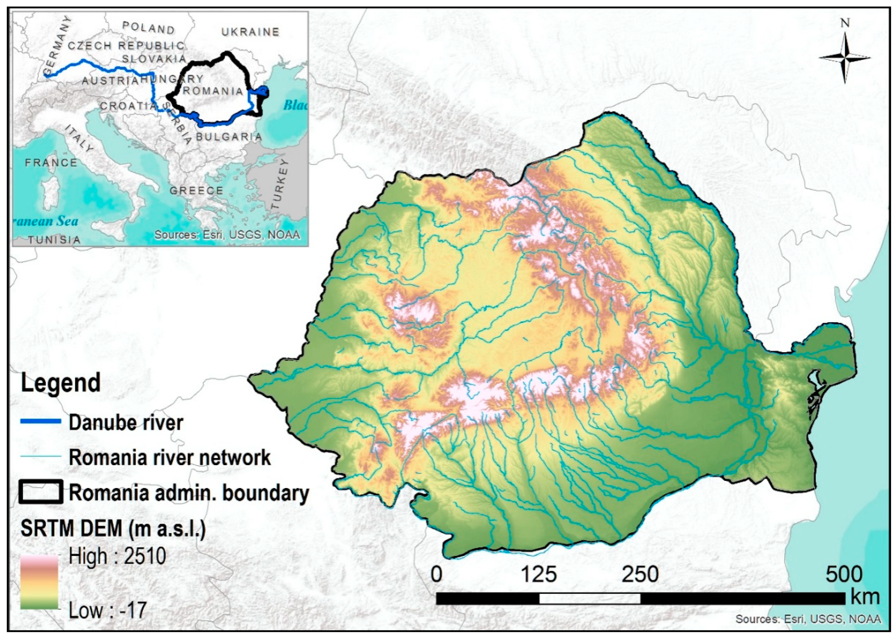
3. Case Study
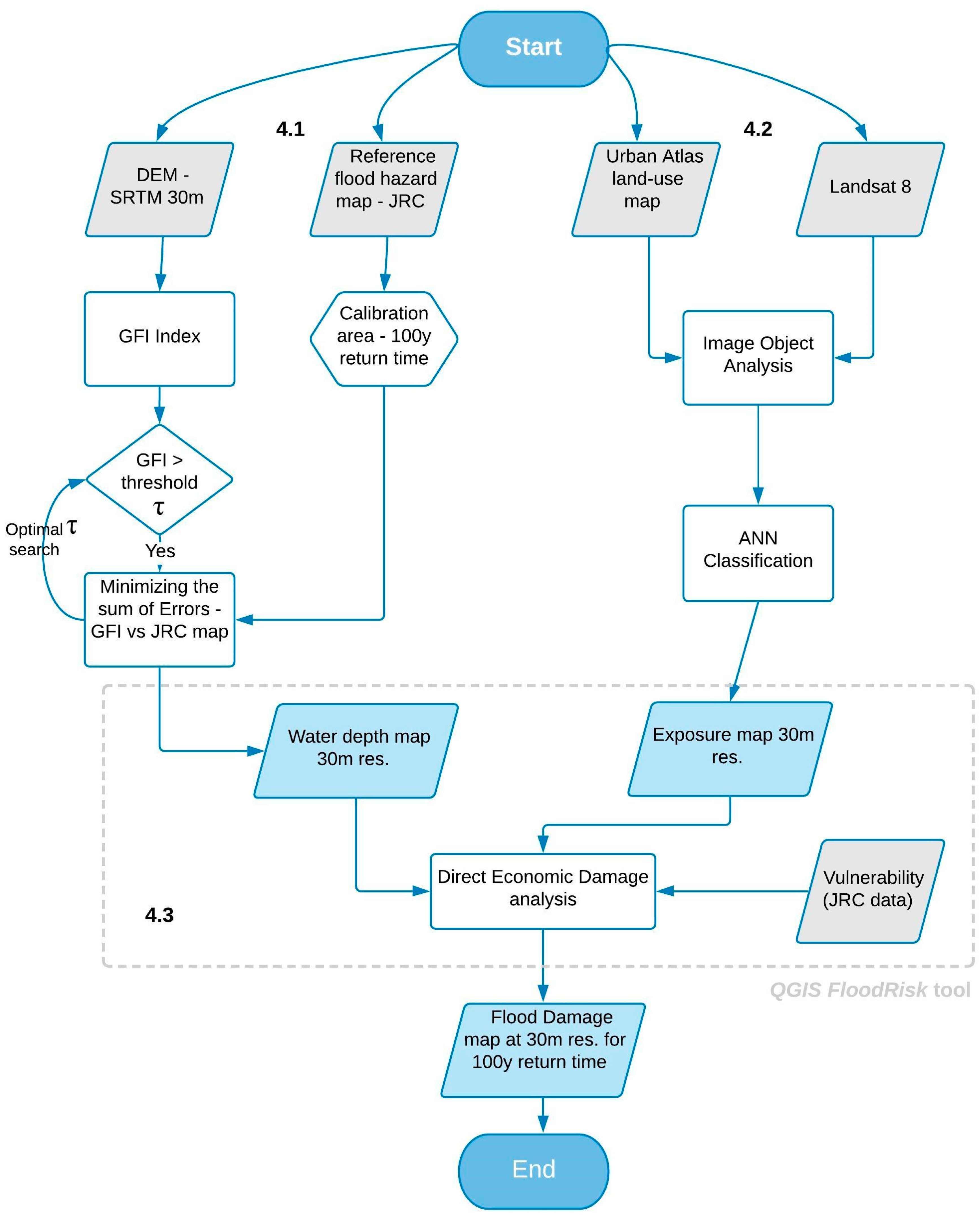
4. Methodology
4.1. Flood Hazard Analysis
4.2. Exposure Analysis
4.2.1. Image Segmentation
4.2.2. Feature-Based Description
4.2.3. Classification
4.3. Damage Analysis
5. Results of the Application in Romania
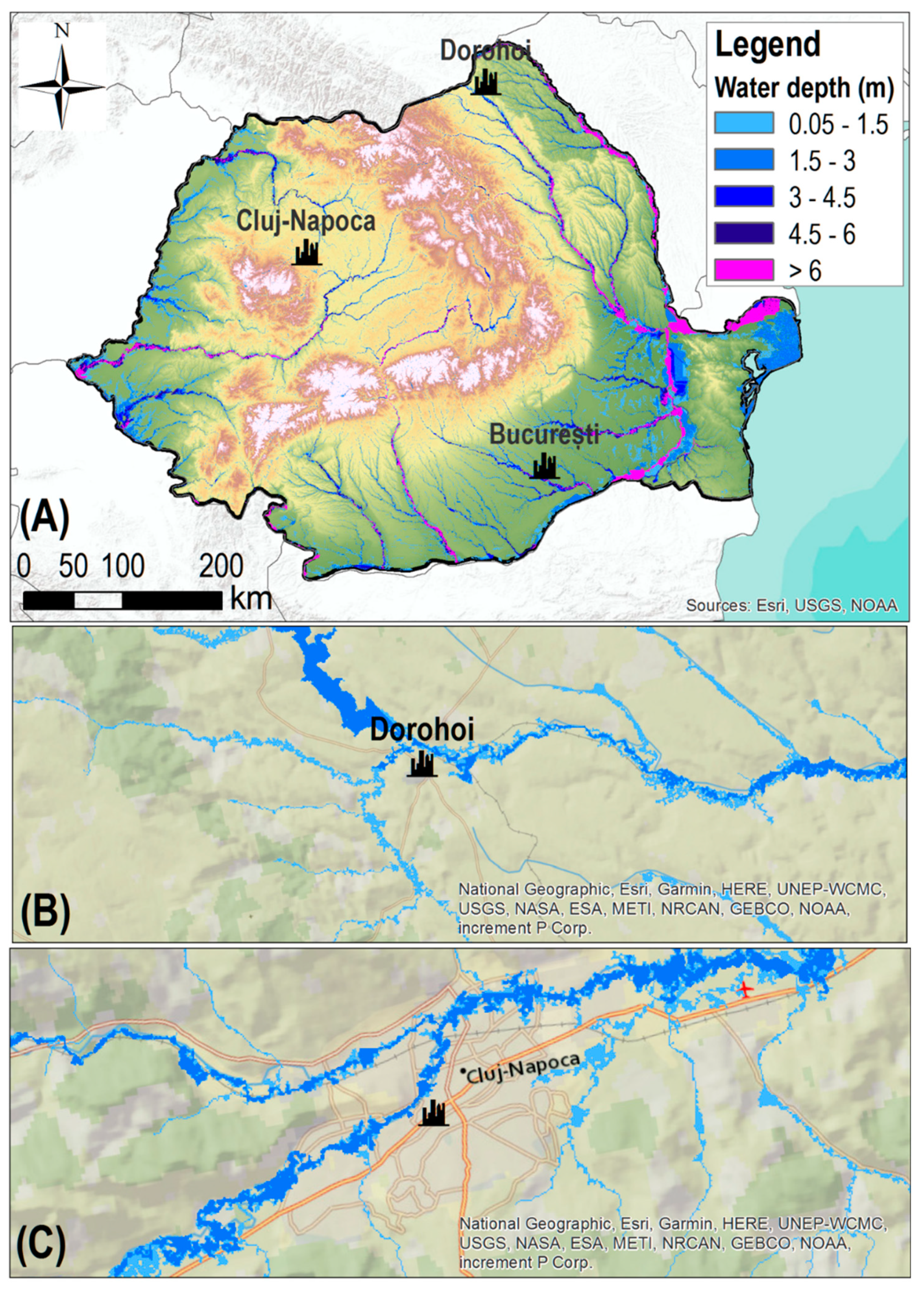
5.1. Flood Hazard Mapping in Romania
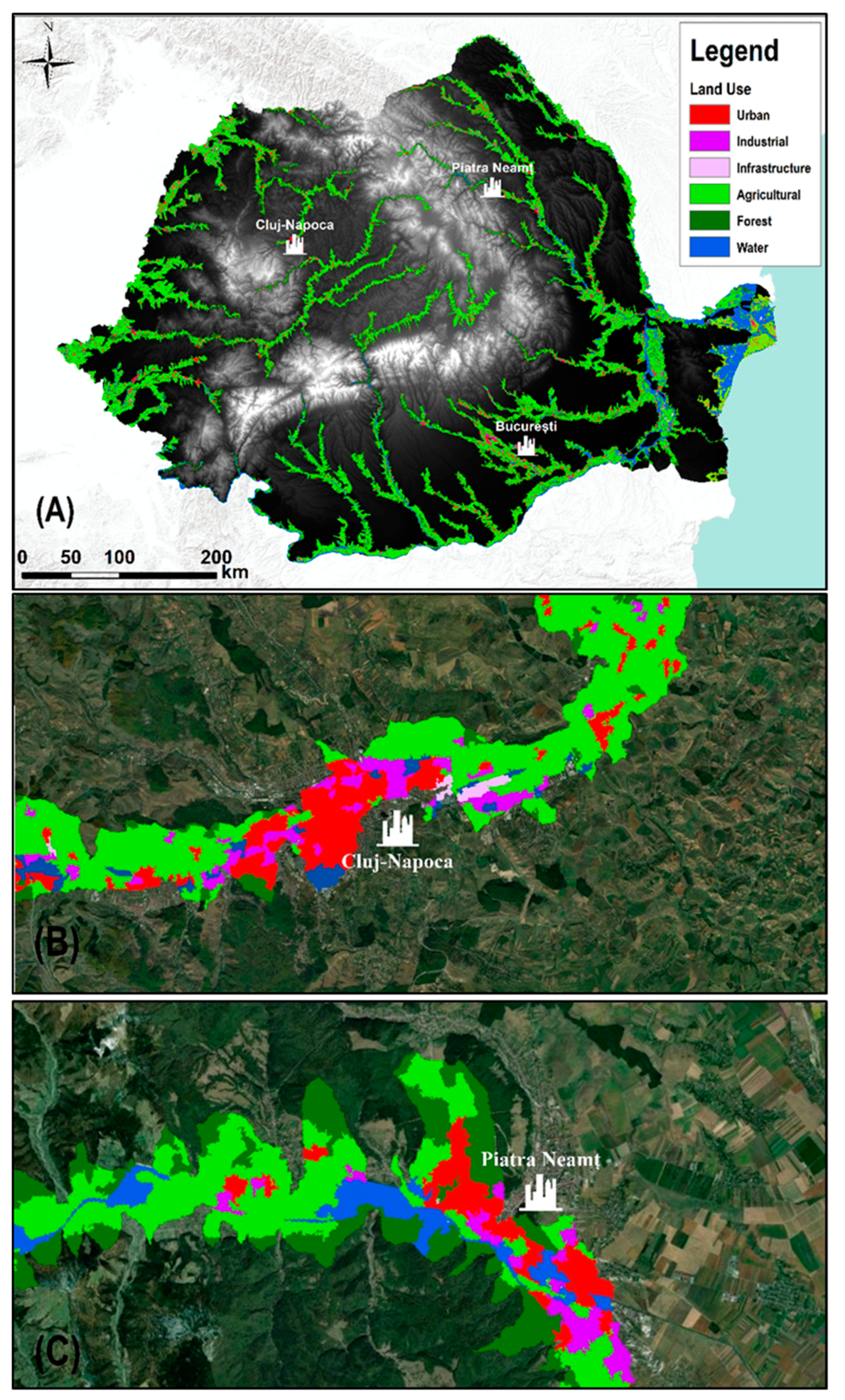
5.2. Exposure Mapping in the Case Study
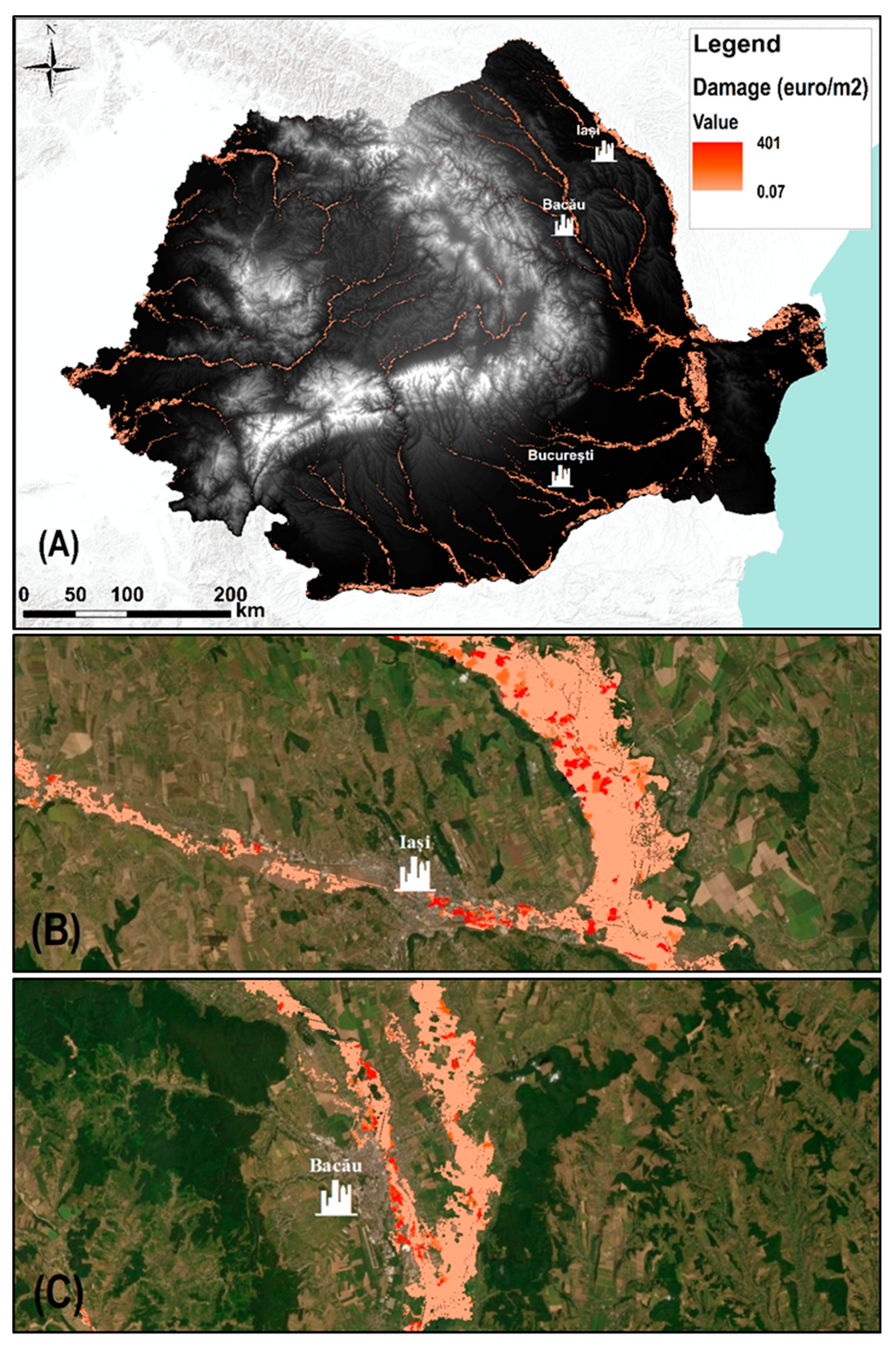
5.3. Economic Damage Mapping of Romania
6. Conclusions
Author Contributions
Funding
Conflicts of Interest
References
- Merz, B.; Kreibich, H.; Schwarze, R.; Thieken, A. Review article-Assessment of economic flood damage. Nat. Hazards Earth Syst. Sci. 2010, 10, 1697–1724. [Google Scholar] [CrossRef]
- Meyer, V.; Becker, N.; Markantonis, V.; Schwarze, R.; van den Bergh, J.C.J.M.; Bouwer, L.M.; Bubeck, P.; Ciavola, P.; Genovese, E.; Green, C.; et al. Review article: Assessing the costs of natural hazards–state of the art and knowledge gaps. Nat. Hazards Earth Syst. Sci. 2013, 13, 1351–1373. [Google Scholar] [CrossRef]
- Dottori, F.; Figueiredo, R.; Martina, M.L.V.; Molinari, D.; Scorzini, A.R. INSYDE: A synthetic, probabilistic flood damage model based on explicit cost analysis. Nat. Hazards Earth Syst. Sci. 2016, 16, 2577–2591. [Google Scholar] [CrossRef] [Green Version]
- IPCC AR4 SYR; Core Writing Team; Pachauri, R.K.; Reisinger, A. (Eds.) Contribution of Working Groups I, II and III to the Fourth Assessment Report (AR4) of the Intergovernmental Panel on Climate Change. In Climate Change 2007: Synthesis Report (SYR); IPCC: Geneva, Switzerland, 2007; ISBN 978-92-9169-122-7. [Google Scholar]
- IPCC 2007. Contribution of Working Group II to the Fourth Assessment Report of the Intergovernmental Panel on Climate Change; Parry, M.L., Canziani, O.F., Palutikof, J.P., van der Linden, P.J., Hanson, C.E., Eds.; Climate Change 2007: Impacts, Adaptation and Vulnerability; Cambridge University Press: Cambridge, UK; New York, NY, USA, 2007. [Google Scholar]
- Albano, R.; Mancusi, L.; Sole, A.; Adamowski, J. Sustainable and collaborative strategies for EU flood risk management: FOSS and Geospatial Tools–challenge and opportunities for operative risk analysis. ISPRS Int. J. Geo-Inf. 2015, 4, 2704–2727. [Google Scholar] [CrossRef]
- Albano, R.; Mancusi, L.; Abbate, A. Improving Flood Risk Analysis for effectively supporting the implementation of flood risk management plans: The case study of “Serio” Valley. Environ. Sci. Policy 2017, 75, 158–172. [Google Scholar] [CrossRef]
- Messner, F.; Meyer, V. Flood damage, vulnerability and risk perception: Challenges for flood damage research. In Flood Risk Management: Hazards, Vulnerability and Mitigation Measures; Schanze, J., Zeman, E., Marsalek, J., Eds.; Springer: Dordrecht, The Netherlands, 2006; Volume 67, pp. 149–167. [Google Scholar]
- European Parliament and the Council of 23 October 2007 on the assessment and management of flood risks. Directive 2007/60/EC. Off. J. Eur. Union 2007, 1, L288/27–L288/34.
- Cirella, G.T.; Semenzin, E.; Critto, A.; Marcomini, A. Natural Hazard Risk Assessment and Management Methodologies. Review: Europe. In Sustainable Cities and Military Installations; Linkov, I., Ed.; Springer: Dordrecht, The Netherlands, 2014; pp. 329–358. [Google Scholar]
- Scorzini, A.R.; Frank, E. Flood damage curves: New insights from the 2010 flood in Veneto, Italy. J. Flood Risk Manag. 2015, 10, 381–392. [Google Scholar] [CrossRef]
- Albano, R.; Sole, A.; Adamowski, J.; Mancusi, L. A GIS-based model to estimate flood consequences and the degree of accessibility and operability of strategic emergency response structures in urban areas. Nat. Hazards Earth Syst. Sci. 2014, 14, 2847–2865. [Google Scholar] [CrossRef] [Green Version]
- Hall, J.W.; Meadowcroft, I.C.; Sayers, P.B.; Bramley, M.E. Integrated Flood Risk Management in England and Wales. Nat. Hazards Rev. 2003, 3, 126–135. [Google Scholar] [CrossRef]
- Hooijer, A.; Klijn, F.; Pedroli, B.; Van Os, A. Towards Sustainable Flood Risk Management in the Rhine and Meuse River Basins: Synopsis of the Findings of IRMA-SPONGE. River Res. Appl. 2004, 20, 343–357. [Google Scholar] [CrossRef]
- Dottori, F.; Kalas, M.; Salamon, P.; Bianchi, A.; Alfieri, L.; Feyen, L. An operational procedure for rapid flood risk assessment in Europe. Nat. Hazards Earth Syst. Sci. 2017, 17, 1111–1126. [Google Scholar] [CrossRef] [Green Version]
- Perrone, A.; Inam, A.; Albano, R.; Adamowski, J.; Sole, A. A participatory system dynamics modeling approach to facilitate collaborative flood risk management: A case study in the Bradano River (Italy). J. Hydrol. 2020, 580, 124354. [Google Scholar] [CrossRef]
- de Moel, H.; Jongman, B.; Kreibich, H.; Merz, B.; Penning-Rowsell, E.; Ward, P.J. Flood risk assessment at different spatial scales. Mitig. Adapt. Strateg. Glob. Change 2015, 20, 865–890. [Google Scholar] [CrossRef] [PubMed] [Green Version]
- Alfieri, L.; Salamon, P.; Bianchi, A.; Neal, J.; Bates, P.; Feyen, L. Advances in pan-European flood hazard mapping. Hydrol. Process 2014, 28, 4067–4077. [Google Scholar] [CrossRef]
- De Roo, A.; Barredo, J.I.; Lavalle, C.; Bodis, K.; Bonk, R. Potential flood hazard and risk mapping at pan-European scale. In Digital Elevation Modelling–Development and Applications in a Policy Support Environment; Peckham, R., Jordan, G., Eds.; Springer: Berlin/Heidelberg, Germany, 2006; pp. 183–202. [Google Scholar]
- Scarpino, S.; Albano, R.; Cantisani, A.; Mancusi, L.; Sole, A.; Milillo, G. Multitemporal SAR Data and 2D Hydrodynamic Model Flood Scenario Dynamics Assessment. ISPRS Int. J. Geo-Inf. 2018, 7, 105. [Google Scholar] [CrossRef] [Green Version]
- Albano, R.; Sole, A.; Adamowski, J. READY: A web-based geographical information system for enhanced flood resilience through raising awareness in citizens. Nat. Hazards Earth Syst. Sci. 2015, 15, 1645–1658. [Google Scholar] [CrossRef] [Green Version]
- Albano, R.; Sole, A. Geospatial Methods and Tools for Natural Risk Management and Communications. ISPRS Int. J. Geo-Inf. 2018, 7, 470. [Google Scholar] [CrossRef] [Green Version]
- Nardi, F.; Vivoni, E.R.; Grimaldi, S. Investigating a floodplain scaling relation using a hydrogeomorphic delineation method. Water Resour. Res. 2006, 42, W09409. [Google Scholar] [CrossRef]
- Rennó, C.D.; Nobre, A.D.; Cuartas, L.A.; Soares, J.V.; Hodnett, M.G.; Tomasella, J.; Waterloo, M.J. HAND, a new terrain descriptor using SRTM-DEM: Mapping terra-firme rainforest environments in Amazonia. Remote Sens. Environ. 2008, 112, 3469–3481. [Google Scholar] [CrossRef]
- Degiorgis, M.; Gnecco, G.; Gorni, S.; Roth, G.; Sanguineti, M.; Taramasso, A.C. Classifiers for the detection of flood-prone areas using remote sensed elevation data. J. Hydrol. 2012, 470–471, 302–315. [Google Scholar] [CrossRef]
- Manfreda, S.; Di Leo, M.; Sole, A. Detection of Flood Prone Areas using Digital Elevation Models. J. Hydrol. Eng. 2011, 16, 781–790. [Google Scholar] [CrossRef]
- Manfreda, S.; Nardi, F.; Samela, C.; Grimaldi, S.; Taramasso, A.C.; Roth, G.; Sole, A. Investigation on the use of geomorphic approaches for the delineation of flood prone areas. J. Hydrol. 2014, 517, 863–876. [Google Scholar] [CrossRef]
- Dottori, F.; Martina, M.L.V.; Figueiredo, R. A methodology for flood susceptibility and vulnerability analysis in complex flood scenarios. J. Flood Risk Manag. 2018, 11, S632–S645. [Google Scholar] [CrossRef]
- Manfreda, S.; Samela, C.; Sole, A.; Fiorentino, M. Flood-prone Areas Assessment Using Linear Binary Classifiers based on Morphological Indices. In Vulnerability, Uncertainty, and Risk Quantification, Mitigation, and Management; ASCE: Washington, DC, USA, 2014; pp. 2002–2011. [Google Scholar]
- Manfreda, S.; Samela, C.; Gioia, A.; Consoli, G.G.; Iacobellis, V.; Giuzio, L.; Cantisani, A.; Sole, A. Flood-prone areas assessment using linear binary classifiers based on flood maps obtained from 1D and 2D hydraulic models. Nat. Hazards 2015, 79, 735–754. [Google Scholar] [CrossRef]
- Samela, C.; Troy, T.J.; Manfreda, S. Geomorphic classifiers for flood-prone areas delineation for data-scarce environments. Adv. Water Resour. 2017, 102, 13–28. [Google Scholar] [CrossRef]
- Manfreda, S.; Samela, C. A digital elevation model-based method for a rapid estimation of flood inundation depth. J. Flood Risk Manag. 2019, 12, e12541. [Google Scholar] [CrossRef] [Green Version]
- Albano, R.; Craciun, I.; Mancusi, L.; Sole, A.; Ozunu, A. Flood damage assessment and uncertainty analysis: The case study of 2006 flood in Ilișua Basin in Romania. Carpath. J. Earth Environ. 2017, 12, 335–346. [Google Scholar]
- Molinari, D.; Scorzini, A.R.; Gallazzi, A.; Ballio, F. AGRIDE-c, a conceptual model for the estimation of flood damage to crops: Development and implementation. Nat. Hazards Earth Syst. Sci. 2019, 19, 2565–2582. [Google Scholar] [CrossRef] [Green Version]
- Albano, R.; Sole, A.; Adamowski, J.; Perrone, A.; Inam, A. Using FloodRisk GIS freeware for uncertainty analysis of direct economic flood damages in Italy. Int. J. Appl. Earth Obs. 2018, 73, 220–229. [Google Scholar] [CrossRef]
- Messner, F.; Pennning-Rowsell, E.C.; Green, C.; Meyer, V.; Tunstall, S.M.; Van der Veen, A. Evaluating Flood Damages: Guidance and Recommendations on Principles and Methods, FLOODsite, Report No. T09-06-01 2007; FLOODsite: Lakitelek, Tiszakécske, 2007. [Google Scholar]
- Kreibich, H.; Seifert, I.; Merz, B.; Thieken, A.H. Development of FLEMOcs–a new model for the estimation of flood losses in the commercial sector. Hydrol. Sci. J. 2010, 55, 1302–1314. [Google Scholar] [CrossRef]
- Kok, M.; Huizinga, J.; Vrouwenvelder, A.C.W.M.; Barendregt, A. Standard Method 2004. In Damage and Casualties Caused by Flooding; Road and Hydraulic Engineering Institute: Delft, The Netherlands, 2005. [Google Scholar]
- de Bruijn, K.; Klijn, F.; Ölfert, A.; Penning-Rowsell, E.; Simm, J.; Wallis, M. Flood Risk Assessment and Flood Risk Management. An Introduction and Guidance Based on Experiences and Findings of FLOODsite; Delft Hydraulics: Delft, The Netherland, 2009; pp. 5–127. [Google Scholar]
- Huizinga, H.J. Flood damage functions for EU member states. In HKV Consultants, Implemented in the Framework of the Contract #382442-F1SC Awarded by the European Commission; Tech. rep.; European Commission-Joint Research Center: Brussels, Belgium, 2007. [Google Scholar]
- Huizinga, H.J.; de Moel, H.; Szewczyk, W. Global Flood Depth-Damage Functions. Methodology and the Database with Guidelines; Publications Office of the European Union: Luxembourg, 2017; pp. 3–108. [Google Scholar]
- Albano, R.; Mancusi, L.; Sole, A.; Adamowski, J. FloodRisk: A collaborative free and open-source software for flood risk analysis. Geomat. Nat. Haz. Risk 2017, 8, 1812–1832. [Google Scholar] [CrossRef] [Green Version]
- Bhatti, S.S.; Abd Tripathi, N.K. Built-up area extraction using Landsat 8 OLI imagery. Gisci. Remote Sens. 2014, 51, 445–467. [Google Scholar] [CrossRef] [Green Version]
- Wieland, M.; Pittore, M. Performance Evaluation of Machine Learning Algorithms for Urban Pattern Recognition from Multi-spectral Satellite Images. Remote Sens. 2014, 6, 2912–2939. [Google Scholar] [CrossRef] [Green Version]
- Wieland, M.; Pittore, M. Large-area settlement pattern recognition from Landsat-8 data. ISPRS J. Photogramm. Remote Sens. 2016, 119, 294–308. [Google Scholar] [CrossRef]
- CRED EM-DAT, Centre for Research on the Epidemiology of Disasters. The International Disaster Database. Available online: www.emdat.be (accessed on 6 February 2019).
- Arghiuș, V.; Botezan, C.; Gagiu, A.C.; Samara, I.; Senzaconi, F.; Ozunu, A. Normalized economical flood damages in Romania during 2000–2009. Environ. Eng. Manag. J. 2011, 10, 17–21. [Google Scholar] [CrossRef]
- Samela, C.; Albano, R.; Sole, A.; Manfreda, S. A GIS tool for cost-effective delineation of flood-prone areas. Comput. Environ. Urban 2018, 70, 43–52. [Google Scholar] [CrossRef]
- Popovici, E.A.; Bălteanu, D.; Kucsicsa, G. Utilizarea terenurilor și dezvoltarea actuală a agriculturii. In România. Natură și Societate; Bălteanu, D., Ed.; Academiei Române: București, Romania, 2016; pp. 329–375. [Google Scholar]
- EEA. Romania Land Cover Country Fact Sheet 2012. 2012. Available online: https://www.eea.europa.eu/themes/landuse/land-cover-country-fact-sheets/ro-romania-landcover-2012.pdf/view (accessed on 20 March 2020).
- Van Zyl, J.J. The Shuttle Radar Topography Mission (SRTM): A breakthrough in remote sensing of topography. Acta Astronaut. 2011, 48, 559–565. [Google Scholar]
- USGS, Landsat Missions. Landsat 8 Data Users Handbook. Available online: https://landsat.usgs.gov/landsat-8-l8-data-users-handbook (accessed on 21 April 2019).
- EEA. Mapping Guide for a European Urban Atlas. 2011. Available online: http://www.eea.europa.eu/data-and-maps/data/urban-atlas (accessed on 3 June 2019).
- Leopold, L.B.; Wolman, M.G.; Miller, J.P. Fluvial Processes in Geomorphology; WH Freeman: San Francisco, CA, USA, 1964. [Google Scholar]
- Pittore, M.; Wieland, M.; Fleming, K. Perspectives on global dynamic exposure modelling for geo-risk assessment. Nat. Hazards 2017, 86, 7–30. [Google Scholar] [CrossRef]
- Giri, C.; Pengra, B.; Long, J.; Loveland, T.R. Next generation of global land cover characterization, mapping, and monitoring. Int. J. Appl. Earth Observ. Geoinf. 2013, 25, 30–37. [Google Scholar] [CrossRef]
- Woodcock, C.E.; Allen, R.; Anderson, M.; Belward, A.; Bindschadler, R.; Cohen, W.; Gao, F.; Goward, S.N.; Helder, D.; Helmer, E.; et al. Free access to Landsat imagery. Science 2008, 320, 1011. [Google Scholar] [CrossRef]
- Zhu, Z.; Fu, Y.; Woodcock, C.E.; Olofsson, P.; Vogelmann, J.E.; Holden, C.; Wang, M.; Dai, S.; Yu, Y. Including land cover change in analysis of greenness trends using all available Landsat 5, 7, and 8 images: A case study from Guangzhou, China (2000–2014). Remote Sens. Environ. 2016, 185, 243–257. [Google Scholar] [CrossRef] [Green Version]
- Benediktsson, J.A.; Sveinsson, J.R. Feature extraction for multisource data classification with artificial neural networks. Int. J. Remote Sens. 1997, 18, 727–740. [Google Scholar] [CrossRef]
- Kavzoglu, T.; Mather, P.M. The use of backpropagating artificial neural networks in land cover classification. Int. J. Remote Sens. 2003, 24, 4907–4938. [Google Scholar] [CrossRef]
- Lu, D.; Weng, Q. A Survey of Image Classification Methods and Techniques for Improving Classification Performance. Int. J. Remote Sens. 2007, 28, 823–870. [Google Scholar] [CrossRef]
- Kuemmerle, T.; Radeloff, V.C.; Perzanowski, K.; Hostert, P. Cross-border comparison of land cover and landscape pattern in Eastern Europe using a hybrid classification technique. Remote Sens. Environ. 2006, 103, 449–464. [Google Scholar] [CrossRef]
- Dingle Robertson, L.; King, D.J. Comparison of pixel- and object-based classification in land cover change mapping. Int. J. Remote Sens. 2011, 32, 1505–1529. [Google Scholar] [CrossRef]
- Phiri, D.; Morgenroth, J. Developments in Landsat Land Cover Classification Methods: A Review. Remote Sens. 2017, 9, 967. [Google Scholar] [CrossRef] [Green Version]
- Felzenszwalb, P.; Huttenlocher, D. Efficient Graph-Based Image Segmentation. Int. J. Comput. Vis. 2004, 59, 167–181. [Google Scholar] [CrossRef]
- Johnson, B.; Xie, Z. Unsupervised image segmentation evaluation and refinement using a multi-scale approach. ISPRS J. Photogramm. Remote Sens. 2011, 66, 473–483. [Google Scholar] [CrossRef]
- Guyon, I.; Weston, J.; Barnhill, S.; Vapnik, V. Gene selection for cancer classification using support vector machines. Mach. Learn. 2002, 46, 389–422. [Google Scholar] [CrossRef]
- Rumelhart, D.E.; Hinton, G.E.; Williams, R.J. Learning representations by back-propagating errors. Nature 1986, 323, 533–536. [Google Scholar] [CrossRef]
- Yoshida, T.; Omatu, S. Neural network approach to land cover mapping. IEEE Trans. Geosci. Remote Sens. 1994, 32, 1103–1109. [Google Scholar] [CrossRef]
- Rodriguez, E.; Morris, C.S.; Belz, J.E. A global assessment of the SRTM performance. Photogramm. Eng. Remote Sens. 2006, 72, 249–260. [Google Scholar] [CrossRef] [Green Version]
- Annis, A.; Nardi, F.; Morrison, R.R.; Castelli, F. Investigating hydrogeomorphic floodplain mapping performance with varying DTM resolution and stream order. Hydrol. Sci. J. 2019, 64, 525–538. [Google Scholar]
- Tavares da Costa, R.; Manfreda, S.; Luzzi, V.; Samela, C.; Mazzoli, P.; Castellarin, A.; Bagli, S. A web application for hydrogeomorphic flood hazard mapping. Environ. Model. Softw. 2019, 118, 172–186. [Google Scholar] [CrossRef] [Green Version]
- Copernicus, Land Monitoring Service, Urban Atlas. Available online: https://land.copernicus.eu/local/urban-atlas (accessed on 25 February 2019).
- Congalton, R.G. A review of assessing the accuracy of classifications of remotely sensed data. Remote Sens. Environ. 1991, 37, 35–46. [Google Scholar] [CrossRef]
- Copernicus, Land Monitoring Service, Corine Land Cover. Available online: http://land.copernicus.eu/pan-european/corine-land-cover (accessed on 25 February 2019).
- Wing, O.; Bates, P.; Sampson, C.; Smith, A.; Johnson, K.; Erickson, T. Validation of a 30m resolution flood hazard model of the conterminous United States. Water Resour. Res. 2017, 53, 7968–7986. [Google Scholar] [CrossRef]
- Sampson, C.C.; Smith, A.M.; Bates, P.B.; Neal, J.C.; Alfieri, L.; Freer, J.E. A high-resolution global flood hazard model. Water Resour. Res. 2015, 51, 7358–7381. [Google Scholar] [CrossRef] [Green Version]


| Image Feature | Features Class |
|---|---|
| Mean spectral value in image bands 1, 2, 4, 5, 6, 7; | Spectral |
| Standard deviation in image bands 1, 3; | Spectral |
| Weighted brightness, with I being the number of image bands, J being the number of pixels per segment and p being the brightness value of the pixels; | Spectral |
| Minimum brightness value in image bands 1, 3, 9, 10; | Spectral |
| Maximum brightness value in image bands 1, 4, 6, 9, 10; | Spectral |
| Mean value of normalized difference vegetation index (NDVI) NDVI = (NIR − Red)/(NIR + Red); | Band index |
| Mean value of normalized difference water index (NDWI) NDWI = (Green − NIR)/(Green + NIR); | Band index |
| Mean value of modified normalized difference water index (MNDWI) MNDWI = (Green − SWIR)/(Green + SWIR); | Band index |
| Mean value of soil adjusted vegetation index (SAVI), where L (here equal to 0.5) is the soil brightness correction factor ; | Band index |
| Mean and standard deviation value of normalized difference built-up index (NDBI) NDBI = (SWIR − NIR)/(SWIR + NIR); | Band index |
| Angular Second Moment derived from the GLCM in band 7; | Textural |
| Dissimilarity derived from the GLCM in bands 1, 2, 6; | Textural |
| Contrast derived from GLCM in bands 1, 2, 4, 7; | Textural |
| Homogeneity derived from the GLCM in bands 1, 4, 6; | Textural |
| Mean derived from the GLCM in bands 1, 3, 4, 5, 6, 7, 9, 10; | Textural |
| Variance derived from the GLCM in band 10; | Textural |
| Basin | τ | Scale Factor a |
|---|---|---|
| 1 | 1.561 | 0.21 |
| 2 | 1.269 | 0.281 |
| 3 | 3.91 | 0.02 |
| 4 | 1.176 | 0.309 |
| 5 | 1.165 | 0.312 |
| Urban | Industrial | Infrastructure | Agricultural | Forest | Water | User’s Accuracy (%) | |
|---|---|---|---|---|---|---|---|
| Urban | 51,398 | 3101 | 175 | 4421 | 0 | 358 | 86.5% |
| Industrial | 2379 | 43,008 | 1153 | 13,116 | 32 | 1002 | 70.9% |
| Infrastructure | 1881 | 3226 | 7526 | 5739 | 70 | 525 | 39.7% |
| Agricultural | 16,339 | 11,868 | 5792 | 379,258 | 234 | 6755 | 90.2% |
| Forest | 1314 | 2094 | 646 | 1165 | 15,794 | 625 | 73.0% |
| Water | 467 | 5362 | 3772 | 6260 | 0 | 64,998 | 80.4% |
| Producer’s accuracy (%) | 69.7% | 61.7% | 39.5% | 92.5% | 96.7% | 87.5% |
| Code | Land Use Class | Adjusted Assets Value (Euro/m2) |
|---|---|---|
| 11100 | Urban | 495 |
| 12100 | Industrial | 667 |
| 12220 | Infrastructure | 11.2 |
| 20000 | Agricultural | 0.07 |
| 30000 | Forest | 0.04 |
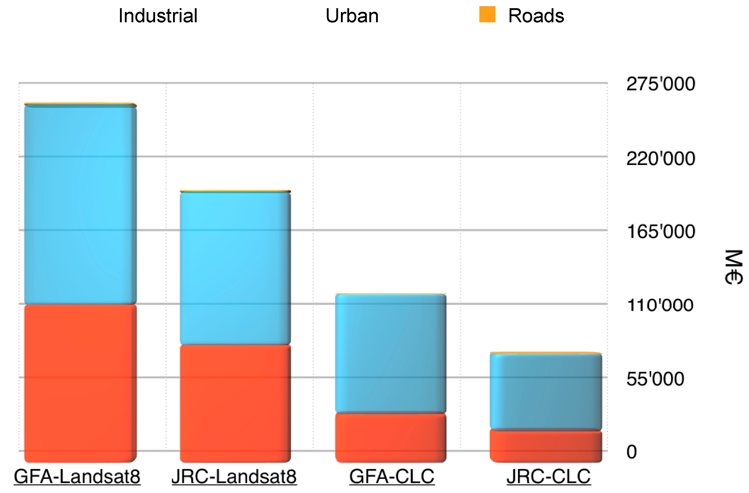
| Economic Flood Damage (M€) | |||||
|---|---|---|---|---|---|
| GFA_Landsat8 | JRC_Landsat8 | GFA_CLC | JRC_CLC | ||
| Land Use Class | Urban | 140,674.86 | 107,996.13 | 84,299.48 | 54,422.28 |
| Industrial | 111,012.6115 | 82,446.2972 | 34,116.04 | 22,025.98 | |
| Roads | 1143.17 | 1100.11 | 74.78 | 57.72 | |
| Agricultural | 444.30 | 399.11 | 536.24 | 507.55 | |
| Forests | 11.78 | 10.92 | 15.68 | 12.71 | |
| Total | 253,286.73 | 191,952.57 | 119,042.22 | 77,026.24 | |
© 2020 by the authors. Licensee MDPI, Basel, Switzerland. This article is an open access article distributed under the terms and conditions of the Creative Commons Attribution (CC BY) license (http://creativecommons.org/licenses/by/4.0/).
Share and Cite
Albano, R.; Samela, C.; Crăciun, I.; Manfreda, S.; Adamowski, J.; Sole, A.; Sivertun, Å.; Ozunu, A. Large Scale Flood Risk Mapping in Data Scarce Environments: An Application for Romania. Water 2020, 12, 1834. https://doi.org/10.3390/w12061834
Albano R, Samela C, Crăciun I, Manfreda S, Adamowski J, Sole A, Sivertun Å, Ozunu A. Large Scale Flood Risk Mapping in Data Scarce Environments: An Application for Romania. Water. 2020; 12(6):1834. https://doi.org/10.3390/w12061834
Chicago/Turabian StyleAlbano, Raffaele, Caterina Samela, Iulia Crăciun, Salvatore Manfreda, Jan Adamowski, Aurelia Sole, Åke Sivertun, and Alexandru Ozunu. 2020. "Large Scale Flood Risk Mapping in Data Scarce Environments: An Application for Romania" Water 12, no. 6: 1834. https://doi.org/10.3390/w12061834