Temperature Extremes: Estimation of Non-Stationary Return Levels and Associated Uncertainties

Abstract

Estimating temperature extremes (TEs) and associated uncertainties under the non-stationary (NS) assumption is a key research question in several domains, including the nuclear safety field. Methods for estimating TEs and associated confidence intervals (CIs) have often been used in the literature but in a stationary context, separately and without detailed comparison. The extreme value theory is often used to assess risks in a context of climate change. It provides an accurate indication of distributions describing the frequency of occurrence of TEs. However, in an NS context, the notion of the return period is not easily interpretable. For instance, to predict a high return level (RL) in a future year, time-varying distributions must be used and compared. This study examines the performance of a new concept to predict RLs in an NS context and compares three methods for constructing the associated CIs (delta, profile likelihood, and parametric bootstrap). The present work takes up the concept of integrated return periods that define the T-year RL as the level for which the expected number of events in a T-year period is one and proposes a new method based on conditional predictions that is useful for predicting high RLs of extreme events in the near future (the 100-year RL in the year 2030, for instance). The daily maximum temperature (DMT) observed at the Orange Station in France was used as a case study. Several trend models were compared and a new likelihood-based method to detect breaks in TEs is proposed. The analyses were conducted assuming the time-varying Generalized Extreme Value (GEV) distribution. The concepts have been implemented in a software package (Non-Stationary Generalized Extreme Value (NSGEV)). The application demonstrates that the RL estimates for NS situations can be quite different from those corresponding to stationary conditions. Overall, the results suggest that the NS analysis can be helpful in making a more appropriate assessment of the risk for periodic safety reviews during the life of a nuclear power plant (NPP).

1. Introduction

Nuclear energy is used to derive over 80% of the electricity in France. Nuclear power plants (NPPs) are not exempt from natural and climatic hazards (flooding, extreme temperatures and heat waves, earthquakes, etc.). The direct, indirect, and cumulative effects of floods, temperature extremes (TEs), and heatwaves impede the safe functioning of NPPs. Nuclear power is a low greenhouse gas emitter but, paradoxically, global warming is making the technology more vulnerable in terms of providing electricity. NPPs in France were constructed to withstand hot summers. In addition, operators are continually investigating prospective internal or external aggressions due to hot temperatures. Nevertheless, climate change and its impact on TEs remain an important issue for the Institute for Radiological Protection and Nuclear Safety (IRSN). During the last two decades, France and other European countries experienced three violent heatwaves (2003, 2006, and 2015) that gave rise to very high temperatures in summer. Urbanization and industrialization, the effect of natural climatic variability, and increased greenhouse gasses in the atmosphere have been suggested as the leading causes of the increase in duration, magnitude, and frequency of TEs and heatwaves in the context of the current climate evolution. Despite the fact that the nuclear facilities were designed to withstand these TEs with a low probability of failure, the current evolution of the climate (global warming) is considered in a too simplistic way by the existing frequency analysis models based on the extreme values theory.

In the current practice using probabilistic methods to estimate design variables, extreme events are generally assumed to be stationary (i.e., in an unchanging climate in a statistical sense) (e.g., [1,2]). The idea that some mechanisms in hydrological systems are time-invariant and the fact that hydrological predictions are based on assumptions that should include stationarity have been argued in the literature (e.g., [3,4,5]). We must keep in mind that these studies emphasize that any hydrological model, including deterministic and nonstationary approaches, is affected by uncertainty and, therefore, should include a random component that is stationary. From these specific studies, however, it is noted that the developments and applications of non-stationary (NS) models in hydrologic frequency analyses in a changing climate and environments can be frustrated when the additional uncertainty related to trend models, for example, is accounted for along with the sampling uncertainty [6].

Nevertheless, many studies in the last few decades have shown that climatic and meteorological records exhibit some type of non-stationarity such as trends and shifts [7,8,9]. Several approaches have been proposed in the literature to tackle non-stationarity in hydrometeorological and climatological extremes. The frequency analysis of TEs with time-varying distribution functions (or moments such as the mean and the variance) is one of the approaches that have been proposed in the literature to characterize TEs in an NS context (e.g., [10,11,12]).

To meet and satisfy safety requirements, estimate return levels with an appropriate confidence level becomes a major operational concern. Definitions of the return period in an NS context, its statistical significance, as well as its interpretation, have to be addressed properly and with extreme care when used for environmental, health, and safety concerns. However, a frequently occurring ‘gap’ is the widespread use of the time-varying frequency models to estimate high return levels (without a projection into the future) while assuming the classic return level concept used in stationary environments: the return level Z_T for T years is the level for which the probability of exceedance every year is equal to 1/T. Nevertheless, the hypothesis allowing the use of this classic definition of the return period T no longer makes sense in an NS case [10,13,14,15,16,17,18,19,20,21,22]. Some early studies on the topic have been described by Wigley [22,23] who presented, in a simple way, how non-stationarity may be considered in the classic concept of risk. Katz et al. [10] proposed the “effective return levels” concept to present non-stationarity in terms of time-varying quantiles while the occurrence probability of an extreme event remains constant. Alternatively, the Design Life Level concept was introduced by Rootzén and Katz [24] to estimate the probability of exceeding a fixed threshold during the design life of a project.

However, even before this, in a paper published in 1941 [25], Emil Gumbel, a pioneer in the field of statistics of extremes, had not only addressed the invalidity of this assumption but also thought about climate evolution that was identified half a century later. He cautioned that:

“In order to apply any theory, we have to suppose that the data are homogeneous, i.e., that no systematical change of climate and no important change in the basin have occurred within the observation period and that no such changes will take place in the period for which extrapolations are made.”

Thus, early on, the use of the extreme values theory was limited by the homogeneity of data and stationarity of both the studied phenomenon (i.e., TEs) and the environment (i.e., an important evolution of urbanization), an issue that will receive attention in the present paper.

Unsurprisingly, some creative ideas have been proposed by researchers for communicating risk and helping to address such an important issue. The most important contributions propose two different definitions of the return period under non-stationarity. The first defines the T-year return level (RL) as the level for which the expected waiting time until the exceedance is T years and proposes the concept of “the expected waiting time before failure” as an equivalent definition of the return period under stationary conditions [18]. More recently, the notion of return period was extended to the NS setting by Parey et al. [19,26]; it defines the T-year RL as the level for which the expected number of events in a T-year period is one. These two definitions suggested by Olsen et al. [18] and Parey et al. [19] for communicating risk were reviewed, compared, and illustrated by Cooley [15] with an application to annual peak flow measurements for the Red River of the North, USA. Obeysekera and Park [17] also used non-stationarity concepts assuming the Generalized Extreme Value (GEV) distribution for estimating sea-level extreme events. The time-varying design level (expressed in return period of extreme events) of coastal facility protection was used. Another concept (replacing the average return period by one) was proposed more recently by Read and Vogel [20]. The authors introduced the reliability (or “risk of failure”) as a new concept to communicate the risk of experiencing an exceedance event within a planning horizon. They defined the risk of failure over a planning period as the likelihood of experiencing at least one event exceeding the design event over a given project life of n years. This approach in a way originated from those proposed by Olsen et al. [18] and Parey et al. [19]. Read and Vogel [20] strongly believe that the probability of failure over an infrastructure’s lifetime (or its associated reliability) is the most important piece of information an engineer can communicate, and rightly so given the huge importance of this information for the public and planners.

A related issue concerns the detection and estimation of break dates in a time series. Indeed, it is commonly known that climate and human activity always has a direct influence on some hydrometeorological processes. Large-scale climatic and oceanic phenomena such as El Niño and the North Atlantic Oscillation (NAO), as well as all kinds of large-scale urbanization and industry projects, may have a direct or indirect impact on some climatic parameters such as ocean and air temperature. Indeed, in addition to the current climatic evolution due to the emission of greenhouse gases into the atmosphere, these particular phenomena are likely to suddenly modify TEs [27]. Therefore, in a context of non-stationarity, identifying abrupt changes in the time series (and locating the times of significant changes) becomes an important step in modeling temporal trends and taking them into account in statistical inference (frequency analysis and associated uncertainties). Various methods have been proposed in the literature for change-point analysis. Non-parametric techniques were introduced for this problem (e.g., [28,29]). Pettitt [28] obtained exact and approximate results for testing the null hypothesis of no change. The study of Servat et al. [29] was based on a set of methods both for interpolation and for cartographic representation, as well as on statistical methods for the detection of breaks in the precipitation time series in Africa. Yu et al. [30] then proposed a general fuzzy piecewise regression analysis with automatic change-point detection. More recently, Xiong and Guo [31] adopted the Bayesian approach to detect a single change in the mean level of both the annual minimum flow series and the annual mean discharge series of the Yangtze River (in China) at the Yichang Hydrological Station. The Bayesian method has the advantage of making inferences on the posterior distribution with respect to change-point location.

Some R-packages have been developed for the analyses of extremes in an NS context exist (e.g., extRemes, GEVcdn, NEVA). The extRemes package [32] is based on the concept of effective return levels and was introduced by Katz et al. [10]. The GEVcdn package [33] supplies a framework for a conditional density estimation network. The package for Non-Stationary Extreme Value Analysis (NEVA) was developed by Cheng et al. [13] to estimate climate extremes using Bayesian inference. The NEVA software provides three approaches for estimating RLs in the NS context: (1) RL (for each return period) with a constant “design exceedance probability” during the lifetime considered for the design; (2) time-varying exceedance probability with constant thresholds; and (3) effective return levels as introduced by Katz et al. [10]. However, these packages do not provide any generalization of the concepts of NS return periods as addressed by Olsen et al. [18] and Parey et al. [18,19].

In this study, a framework for TE analysis under NS conditions is introduced. Based on the concepts proposed by Olsen et al. [18] and Parey et al. [18,19,26], two notions of NS return period have been implemented in a software package called Non-Stationary Generalized Extreme Value (NSGEV). Under the NS assumption, NSGEV provides two different kinds of predictions for estimating return levels in a future year: (a) conditional prediction (CP) in which the RL is conditional to a fixed date (i.e., the future year 2030, for instance); and (b) integrated prediction (IP) in which the RL is integrated over a future period (i.e., the concept introduced by Parey et al. [19,26]). A unique feature of NSGEV is that it provides CIs that are calculated with the three most widely used methods: delta, profile likelihood, and bootstrap. Furthermore, unlike existing tools, calculation of the CIs by profile likelihood is automated in NSGEV. Further noteworthy features of the NSGEV package are that it provides and plots the density functions at any future date, provides the number of exceedances of any extreme temperature (the higher value in observations or the 100-year RL, for instance), and uses the likelihood-based method to detect breaks in climatic and hydrometeorological time series. These features make NSGEV a practical tool that is particularly useful for carrying out expert assessments to characterize climatological and hydrometeorological hazards and analyze extremes in both stationary and NS contexts.

Overall, our goal is to build on the definitions and developments proposed in the literature and revive the debate as to how engineers can effectively communicate the risks associated with climatological and hydrometeorological hazards especially over medium- and short-term planning horizons. This goal is in line with the recent literature that challenges the stationarity assumption and clearly demonstrates the importance of conducting extreme-value analyses in a non-stationary context. In order to achieve this goal, a simple framework to estimate RLs under stationary and NS assumptions is introduced with an application to make it accessible to a broad audience in the field of NS extreme-value analysis and make it easily interpretable by engineers.

The paper is organized as follows: The theoretical basis for these approaches will be addressed in Section 2. The methodology of estimating the trends and break dates detection and estimation shall form the subject of the third section of this paper. Section 4 presents the NSGEV R-package, takes up the concept of integrated return periods introduced by Parey et al. [19,26], and proposes a new one based on conditional predictions. In Section 5 and Section 6, the concepts are applied using the daily maximum temperatures (DMTs) observed at the Orange Station in France as a case study. Finally, we conclude in Section 7 with recommendations concerning suitable statements of the unconditional return periods in non-stationary settings.

2. Extreme Values in a Non-Stationary Environment—Theory

Extreme Value Theory (EVT) is an appropriate framework for analyzing the risks associated with climate extremes and their return levels [10,34]. It is assumed here that the reader is familiar with statistical extreme value analysis using this theory and those who are not are referred to Coles [34]. In this section, we give a very brief background primarily to identify the notation used here. In this section, we give, nevertheless, the theoretical elements necessary for generally understanding the EVT and the concepts and definitions that will be proposed in this paper.

One of the three limiting distributions—Gumbel, Fréchet, or Weibull—is often fitted to environmental time series of extreme values such as annual maxima [35]. These three distributions come from the same family, the generalized extreme value (GEV) distribution. The GEV distribution has been applied in a large number of studies to estimate and analyze extremes [11,35,36,37]. The frequency model using this family of distributions is often referred to as the block maxima approach (e.g., [34]). A similar theory holds for excesses over a high threshold. The peaks-over-threshold (POT) approach in which the excesses are analyzed with the Generalized Pareto (GP) distribution is another widely used frequency model based on the EVT (e.g., [34]). The GEV distribution depends on three parameters: location (µ), scale (σ), and shape (ξ) in a cumulative distribution function expressed as:

$$F\left(x,\mu ,\sigma ,\xi \right)=exp\left\{-{\left[1+\xi \left(\frac{x-\mu }{\sigma }\right)\right]}^{-\raisebox{1ex}{$1$}\!\left/ \!\raisebox{-1ex}{$\xi $}\right.}\right\}$$

(1)

The location parameter specifies the center of the distribution, the scale parameter gives an indication of the size of deviations around the location, and the shape parameter governs the tail behavior of the GEV distribution. For NS processes and environments, it is often necessary to allow the underlying distribution function to be time dependent [14,21,32,38] by allowing its parameters (µ, σ, ξ) to depend on time or other covariates. This is commonly referred to as the time-varying frequency model, which is used as an alternative approach.

3. The Time-Varying Distribution and Methodology for Non-Stationarity

We propose three methodological issues in the present section. First, we use the time-varying GEV distribution to estimate TEs under the non-stationarity assumption. In this first step, trend identification and estimation are also performed. Second, in a context of non-stationarity, it is essential to investigate whether there are sudden changes in the time series and to locate the times of significant changes (e.g., [29]), if any. It is then useful to model the time series with multiple linear trends and propose a method for break date analysis. Third, we estimate the uncertainty by examining CIs for the time-varying GEV parameters and other quantities of interest such as the desired NS-RLs that are usually required for nuclear safety (100-year RL, for instance).

3.1. Time-Varying Distribution

The location and scale parameters are often time-varying (expressed as a function of time t) in the NS-GEV distribution (e.g., [39,40]). Other covariates can also be used [34] (only time is used herein). As is usually done, the location and scale parameters are assumed to be polynomial functions of time to account for non-stationarity (Equation 4) while keeping the shape parameter constant. Indeed, even for the stationary case, reliable estimates of the shape parameter cannot be obtained easily and that is why it is advisable to assume it as a constant (e.g., [11,34]), unless there is a convincing reason to let it be time-varying. Another reason for keeping the shape parameter constant is to reliably model its temporal variability that requires long observation periods (often not available for practical applications). It should be noted that the method developed in the ensuing sections are not constrained by the assumption of the constant shape parameter. The cumulative NS-GEV distribution function is given by the following equation ([34]):

$$F\left(x\hspace{0.17em};\hspace{0.17em}\hspace{0.17em}\mu \left(t\right),\hspace{0.17em}\sigma \left(t\right),\hspace{0.17em}\xi \right)=exp\left\{-{\left[1\hspace{0.17em}+\hspace{0.17em}\xi \left(\frac{x-\mu \left(t\right)}{\sigma \left(t\right)}\right)\right]}^{-\raisebox{1ex}{$1$}\!\left/ \!\raisebox{-1ex}{$\xi $}\right.}\right\}$$

(2)

Many methods for estimating the distribution parameters are available. The most popular include the maximum likelihood (e.g., [34]), probability weighted moments (e.g., [41]), L-moments (e.g., [42]), and Bayesian methods (e.g., [43]). Without carrying out a comparative study of these methods, we merely describe briefly the maximum likelihood method used in the present work. It is commonly known that this approach may give unrealistic estimates for the shape parameter when relatively short samples are used (e.g., [44]). Nevertheless, it remains that for applications on extreme temperatures, enough data are typically available to expect that the maximum likelihood method would be stable. However, more interestingly, this method is applied herein because it allows one to easily incorporate time (or any other covariates) into the parameter estimates. The maximum likelihood method is more straightforward than most of the alternative methods for obtaining error bounds for parameter estimates.

3.2. Estimation of Non-Stationarity and Time-Varying Distribution Parameters

To use the best time-varying GEV distribution, criteria for selecting the best time-varying model among the GEV models that allow non-stationary scale and location parameters are compared. The Akaike information criterion (AIC) and the Bayesian information criterion (BIC) are always used to detect non-stationarity and to select an adequate distribution. In addition, the likelihood ratio test (or the deviance criterion) can be used to compare the fit of two nested models: the stationary case (with likelihood $L\left\{null\right\}$) is represented by the null model whereas the alternative is the NS case ($L\left\{alternative\right\}$). The log-likelihood ratio statistic can be expressed as follows [13,34]:

$$D=-2\ln \left[\frac{L\left\{null\right\}}{L\left\{alternative\right\}}\right].$$

(3)

To analyze low frequency NS TEs, it is useful to detect and estimate the temporal trends. Regression structures allowing quadratic dependence on time can be considered for µ and σ parameters:

$$\{\begin{array}{l}\mu \left(t\right)={\mu }_0+{\mu }_{1}t+{\mu }_2{t}^2\\ \sigma \left(t\right)=\exp \left({\sigma }_0+{\sigma }_{1}t+{\sigma }_2{t}^2\right)\end{array}.$$

(4)

In climate and hydrometeorology literature, linear or log-linear trends are usually preferred when selecting trends in the occurrence of extremes [45]. In this study, only non-stationarity with respect to location and scale parameters is discussed. The simplest case with a linear regression for the location parameter $\mu \left(t\right)={\mu }_0+{\mu }_{1}t$, while keeping the scale and shape parameters constant, has often been considered in the literature (e.g., [14]). Three general trend models are tested:

• $M_1$: only the trend after the break date is considered;
• $M_2$: both trends, before and after the break date, are considered;
• $M_3$: there is no break date: a single trend over the entire dataset.

A trend model is better than another if it is more significant (at 90% and 95% levels). For convenience, only linear models are used for the temporal evolution of DMTs. Trend models are compared using the Akaike and Bayesian information criteria (AIC and BIC). The likelihood ratio test is used as well. For each model $M_i\left(i=1,2,3\right)$, three cases are considered:

• $M_i\left(1,0\right)$: corresponds to an NS linear model for $\mu \left(t\right)$ and a stationary one for $\sigma \left(t\right)$;
• $M_i\left(1,1\right)$: corresponds to an NS linear model for both $\mu \left(t\right)$ and $\sigma \left(t\right)$;
• $M_i\left(0,0\right)$: corresponds to a stationary model for both $\mu \left(t\right)$ and $\sigma \left(t\right)$.

Following the same logic, a model $M\left(1,2\right)$ corresponds to an NS linear model for $\mu \left(t\right)$ and an NS quadratic model for $\log \sigma \left(t\right)$. On the other hand, it is commonly known today that the estimation of the shape parameter ξ may sometimes cause difficulty, as observed by Coles and Dixon [46] who proposed the use of a penalized likelihood function to avoid this problem. Similarly, Martins and Stedinger [47] proposed restricting the estimate of ξ to fall within a restricted range. However, we did not encounter any difficulty in the estimation of ξ in the present work.

3.3. Break Dates

Without claiming a breakpoint, if there were any, the use of a frequency model would be impaired by the use of a single trend representative of all data. Indeed, the use of a single trend, where a trend break exists, would introduce a significant bias in the results. On the other hand, considering the breakpoint and taking into account only the post-break data would significantly reduce the size of the sample and this would be an equally poor solution.

As mentioned in the introductory section, many approaches have been proposed and applied in the literature for change-point analysis [28,29,30,31]. In this study, a new likelihood-based approach was adopted to detect change-points in the temporal evolution of annual maximum temperatures. Unlike existing methods and tests for break-point detection (except for non-parametric tests such as the Pettitt one [28,29]), which generally assume that observations are normally distributed (such as the standard normal homogeneity test (SNHT) introduced by Alexandersson (1986) [48] and the Buishand range test [49]), the likelihood-based method has the advantage of making inferences on extreme value distributions (i.e., GEV, GP). In addition, it allows the use of multiple linear trends and exploits all available data considering the post-break slope, as well as the one prior to the occurrence of each proposed breakpoint. Still, even if this strategy uses the suitable breakpoint of a specific series, it has its limitations. Indeed, it is not uncommon for the slopes on either side of the breaking point to be of opposite signs, i.e., a negative trend before the break and a positive one after. A single and generalized trend model (one trend model for all the data) is adopted in this case (the one after the break, of course). A single trend, as will be shown later in this paper with the case study, should be used if no break date has been identified.

Two types of models can be used. In the first model with one trend, there is only one trend after the break date (and no trend before). In the second model, there can be two different trends, a trend before and a trend after the break date. As mentioned earlier, the break date is determined using the principle of maximum likelihood. Indeed, m models (with a different break for each) are tested where m is the number of years of data available. In the developed procedure, each year of the data period is assumed to be a potential candidate for a break year. Looking through all the years of the period of interest, a log-likelihood profile is computed and plotted. Finally, the maximum of the likelihood profile, corresponding to the most appropriate break date, is extracted. It is to be noted that the developed method that optimizes the breakpoint with the likelihood function by evaluating the most likely break dates is not yet implemented in the NSGEV package.

3.4. Uncertainty Associated with Non-Stationary Extreme Events

Generally, when examining TEs, we are interested in asking the question: How often do we expect a nuclear power plant to experience an extreme temperature? Additionally, if that happens, how high will the temperature be? To answer these questions, we need to calculate the return level for a given return period. The 1/p return level ${\widehat{z}}_p$ (computed from the GEV distribution) is the 1 − p quantile and it is given by:

$${\widehat{z}}_p=\{\begin{array}{l}\widehat{\mu }-\frac{\widehat{\sigma }}{\widehat{\xi }}\left[1-y_p{}^{-\widehat{\xi }}\right]\hspace{0.17em}\hspace{0.17em}\hspace{0.17em}\hspace{0.17em}\hspace{0.17em}\widehat{\xi }\ne 0\\ \widehat{\mu }-\widehat{\sigma }\hspace{0.17em}\log y_p\hspace{0.17em}\hspace{0.17em}\hspace{0.17em}\hspace{0.17em}\hspace{0.17em}\hspace{0.17em}\hspace{0.17em}\hspace{0.17em}\hspace{0.17em}\hspace{0.17em}\hspace{0.17em}\hspace{0.17em}\widehat{\xi }=0\end{array}$$

(5)

where $y_p=-\log \left(1-p\right)$. A degree of uncertainty in the estimates of a return level is then closely related to that of the model parameters. It is a common belief today that a good estimation of uncertainty in extreme levels can be as important as the estimate of the level itself (e.g., [34]). It is then noteworthy that a frequency model predicts well the future return values only if it produces RL estimates that fit inside a CI. Three methods for computing CIs—delta, profile likelihood, and bootstrap—are used here in stationary and NS contexts. Appendix A presents a description of these methods that are quite well documented in the literature. Standard errors (and their corresponding confidence intervals) of the GEV distribution parameters and of return levels of interest were estimated and examined for each method. Despite the fact that the variance and confidence intervals based on the maximum likelihood estimators and delta method are asymptotic, the scientific community no longer has any doubt that parametric confidence intervals based on a normal distribution approximation cannot be expected to be accurate for extremes; that is, their actual coverage probabilities will not be close to the nominal values [50]. Uncertainty in predictions also stems from model selection. The CIs are based on the assumption that the correct model has been selected and take no account of the alternatives that could be considered. Probabilistic approaches exist and are used in many contexts to overcome this objection but are not considered here. To make the best possible use of the expertise, we compare the three methods to best characterize the uncertainties. This comparison, which sometimes leads us to make conservative choices, gives us an indication of the conditions under which one method or another is more appropriate. However, in some cases, the estimation of extreme quantiles can inherently be so uncertain that the discrepancy between different types of confidence intervals is not of major relevance. Furthermore, in the nuclear safety field in France, the 70% confidence interval is considered “reasonable” for most reference situations (as the upper bound of the confidence interval is often involved in the estimation of the return level of interest). It is an expert choice used by French nuclear operators.

4. The NS Return Period—NSGEV Package Features

As explained in the introductory section of the present paper, the definition of the RL (i.e., the T-years RL is the level for which the probability of exceedance is 1/T each year) no longer holds in an NS case. Indeed, depending on the identified temporal trend, the level at which the expected number of its exceedances in the next $T$ years will be one must be defined. In the context of non-stationarity, the RL value varies over time and it is in this perspective that the NSGEV package has been developed. Existing packages (e.g., extRemes, GEVcdn or NEVA) estimating extreme values in an NS context consider time as any other explanatory variable. There is, therefore, no “time-varying” model and this is the object of the NSGEV package. It is developed to estimate and to extrapolate (beyond the observation period) to the desired return level of extreme events and to evaluate the risk associated with the NS phenomena. Time, then, becomes an important variable in the return level equation (model becomes conditioned by time). The initial date and the number of years considered to make the prediction are the two key parameters of the RL equation in an NS context. Therefore, the return level Z_T for T years starting from an initial date t₀ (i.e., 2017) will be defined.

Two notions of the NS return period have been implemented in the NSGEV (two kinds of predictions are allowed):

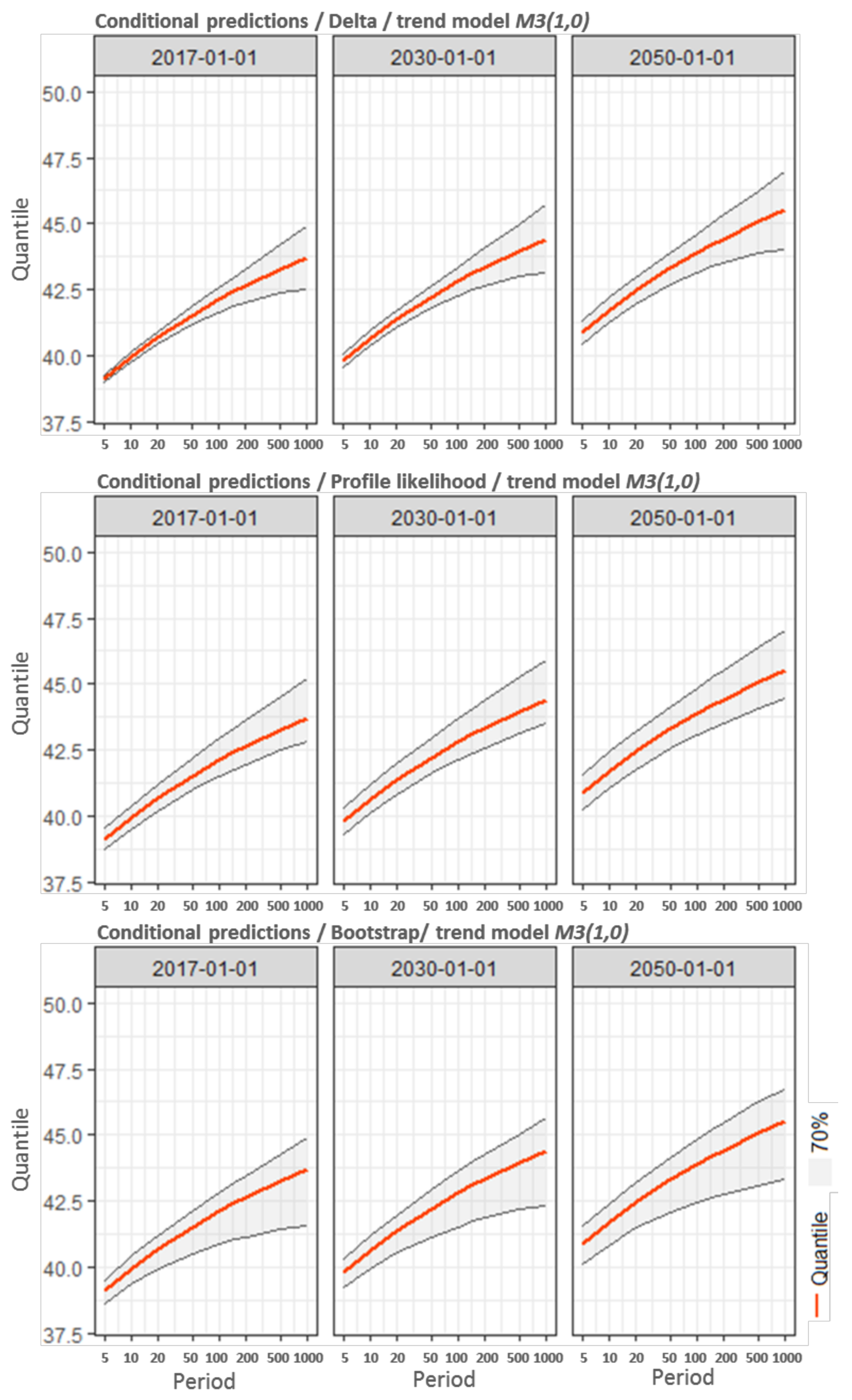
• Return period conditional to a fixed date: relative to a future block (i.e., 2030). It is conditional to the explanatory variable, which is the date of this block. In the introductory section, this is called the conditional prediction (CP).
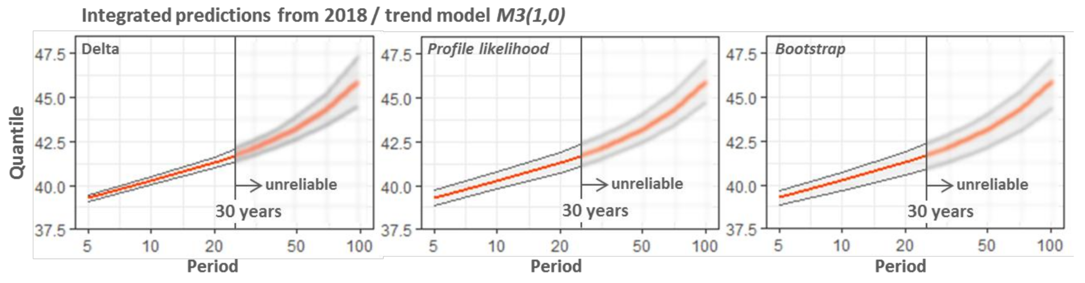
• Return period integrated over a future period: as proposed by Parey et al. [19], the calculated RL corresponds to an expected number of exceedances equal to one over this period. The user must select the first year of the projection and then calculate the predictions for different periods starting from this year. This is what we called the integrated predictions (IP).

One key advantage of the first concept is that, unlike the IP, we do not need to assume that the current trend will remain unchanged until far horizons. Indeed, this is an attractive feature in the analysis and prediction of TEs, especially for those who do not venture into planning and projecting far into the future (i.e., medium and long-term) when dealing with a temperature-related project. Furthermore, for the needs of expertise and periodic evaluations of the safety demonstration of NPPs that operators can put forward, we need to predict high RLs (the 100-year RL, for instance) in the near future (10–30 years, for instance) instead of RLs corresponding to the short-term horizons. That is why the unconditional definition of a return period, as introduced by Parey et al. [19,26], may not be fully relevant for describing the recurrence of extreme temperature events (100-year RLs, for instance) in the near future. Alternatively, the conditional definition, introduced herein, provides high RLs but for reasonable horizons and without making any assumption about the persistence of trends. The two definitions are implemented in NSGEV with the three methods of calculation of the CI: delta, profile likelihood, and bootstrap. Furthermore, unlike existing tools, the calculation of the CIs by the likelihood profile is automated in NSGEV.

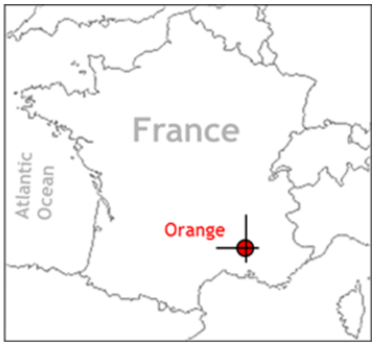
5. Case Study: The Orange Station in France

The TE frequency analysis was performed at the Orange Station, which is located in Southern France. The 1952–2016 DMTs were provided by the French National Meteorological Service (Météo-France). One of the most important features of the Orange Station is the fact that the region in which this station is located has experienced important TEs and heatwave events during the last two decades (e.g., European heatwave of the summer of 2003, the heatwave of the summer of 2006 in Western Europe, and the heatwave of the summer of 2015 in France). Figure 1 displays the geographic location of the Orange Station. The Orange DMT series is considered by Météo-France as homogeneous. It is considered to be one of the best and longest daily data available at Météo-France [19].

As part of a climate watch and a periodic nuclear safety review, all reference extreme temperatures (in all the meteorological stations representative of NPPs in France) are subject to revision. The developed methodology was applied to no fewer than 10 sites, which allowed us to assess the general validity of the methodology. The model was applied in all its stages except in two situations where opposite trends (negative before the breaking points and a positive trend after) were obtained. Only the trend after the breakpoint was considered for these two cases. Aside from the validity of the proposed methodology, the main recommendation of the exercise (in its regional context) was to conduct a more in-depth study to regionalize the trend models.

6. Results and Discussion

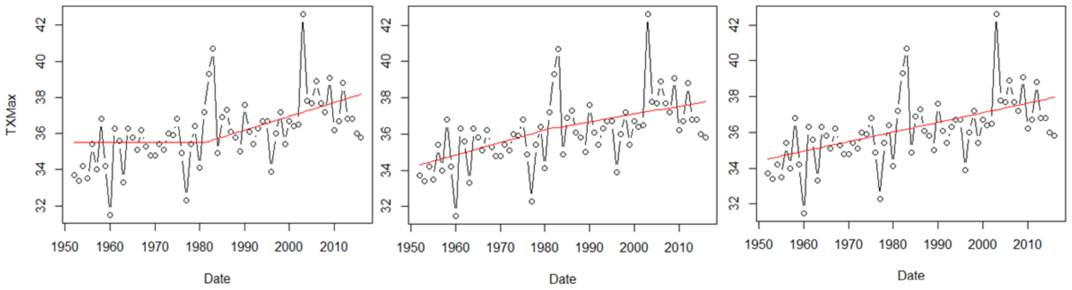
We report herein the results of the conditional and integrated prediction methods applied to the Orange Station. As with any sensitive facility, high return levels (RLs) (the 100-year hot temperature, for instance) in a future year are needed for the safety of NPPs. Furthermore, for the needs of expertise and periodic evaluation of the safety demonstration of NPPs, we need to predict these high RLs with the associated upper bounds of the CIs in a near future (10–30 years, for instance). Despite this, we have taken the liberty to present integrated predictions covering the period up to 2118 (a 100-year NS return period). These results are presented in the form of probability plots and tables summarizing the estimates of the desired RLs and associated CIs calculated using three methods: delta, profile likelihood, and bootstrap. In the probability plots, the time-varying GEV distribution function is represented by the solid red line in the figures while the hatched area represents the 70% CIs. The CPs will first be performed considering three arbitrary dates and then presented. The integrated predictions will be presented afterward. Other features of the NSGEV package, as well as additional results, will likewise be presented. However, even before that, we need to identify and estimate the optimal trend characterizing the TEs at the Orange Station.

6.1. Optimal Trend

For convenience, only linear models are used for the temporal evolution of DMTs. As mentioned above, trend models are compared using the AIC and BIC. The results of the trend estimations are summarized in

Table 1. Trend model comparison with the Akaike information criterion (AIC) and Bayesian information criterion (BIC). Numbers 1 and 0 are the polynomial degrees used in trend models (0 for a stationary model and 1 for a linear model).

	After the Break Date ${\mathit{M}}_{\mathbf{1}}$		Before and After the Break Date ${\mathit{M}}_{\mathbf{2}}$		With No Break Date ${\mathit{M}}_{\mathbf{3}}$
	1	0	1	0	1	0
1	(252.2; 263.1)	(251.0; 259.7)	(246.7; 261.9)	(244.6; 255.5)	(245.1; 256.0)	(243.1; 251.8)
0	*	(267.5; 256.0)	*	(267.5; 256.0)	*	(267.5; 256.0)

* Linear trend on the scale parameter is allowed only if the location parameter is non-stationary (NS).

. The rows in this table correspond to the location parameter $\mu$ and the columns to the scale parameter $\sigma$. The results of the (AIC; BIC) criteria for model $M_i\left(1,1\right)$ are presented in line 1 columns 1, 3, and 5; for model $M_i\left(1,0\right)$ in line 1 columns 2, 4, and 6; and for model $M_i\left(0,0\right)$ in line 2 columns 2, 4, and 6.

The analysis of the results shows that the AIC and BIC give an advantage to the $M_3$ model with an NS linear trend on the location parameter. Furthermore, the outputs of the likelihood ratio test show that the trend model $M_3$ with an NS linear evolution of the location parameter and with no break date (line 1 and column 6 of Table 1) is more significant (at 95% levels). The comparison based on the likelihood ratio statistic give an advantage to the $M_3$ trend model with a p-value equal to 49.33% when compared to the most competitive non-stationary model ($M_2$) with linear trends on location parameter before and after the break date.

The latter result is coherent with those of the NSGEV likelihood-based algorithm to identify breakpoints. Indeed, the plot (not presented herein) of the likelihood as a function of time (candidate break dates) does not present any global extremum likely to correspond to a maximum of likelihood (whose projection on the X-axis gives a potential break date). It should be noted that these results are also consistent with those obtained by Laurent and Parey [51] for the Orange Station. However, this is not entirely consistent with the date of the onset of climate change (the 1970s) commonly shared in the literature and from which trends in extreme temperatures become significant. Figure 2 shows the time evolution of the annual maximum temperatures over the period 1952–2016. The NS linear evolution of the expected value (without any break date) is represented by the straight red line in the figure. Since the density of the annual maximum temperatures is close to that of a GEV distribution of which the parameters were estimated by the maximum-likelihood method, the expectation is given by $\mu +\gamma \sigma$ where $\gamma =0.577$ is the Euler–Mascheroni constant.

6.2. Conditional and Integrated Predictions

A convenient tool for estimating either conditional or integrated predictions is the “predict” function in the package NSGEV. The CP was performed for three dates (2017, 2030, and 2050) and the results are summarized in

Table 2. Results of the conditional predictions (CPs) for the years 2017, 2030, and 2050.

	100-Year RLs (°C)	70% CIs (°C)
		Delta	Profile Likelihood	Bootstrap
2017	42.1	41.6–42.6	41.5–42.9	40.9–42.8
2030	42.8	42.3–43.4	42.1–43.7	41.5–43.6
2050	43.9	43.1–44.6	43.1–44.9	42.4–44.8

and shown in Figure 3. It can be seen that under the non-stationarity assumption, the 100-year return level reaches about 44.0 °C by the year 2050. The results of the CP for the year 2050 are shown in the right panel of Figure 3. In this figure, the CI was calculated with the three methods (delta, profile likelihood, and bootstrap) considering a trend for the period 1952–2016. Looking out to the year 2050, the highest upper bound of the CI around the 100-year return level was obtained by the profile likelihood method and it is equal to 44.9 °C (44.6 °C with the delta method and 44.8 °C with the bootstrap method). For comparison purposes, we also analyzed the same DMT series (for the same period) under the stationarity assumption for which we focused our attention on the 100-year RL and associated CIs. This yields an estimate of 41.1 °C for the 100-year return level and 41.9 °C for the upper bound of the CI calculated with the bootstrap method. The intent of this analysis is only to illustrate how the RL estimates for non-stationary situations can be quite different and significantly larger than those corresponding to stationary conditions. As it can also be noticed in Figure 3, the CIs (calculated with the three methods) are relatively narrow and the relative width $\left(\Delta CIs/RLs\right)$ of these intervals does not exceed 6%. They are likewise very similar and differences in the upper bounds are almost negligible (does not exceed 0.3 °C) for all of the dates.

When the predictions are integrated over a period with a start block date being chosen (say t₀ = 2018), the IPs corresponding to a return period of $T$ years was calculated using the $T$ years from $t_0$ to $t_0+\left(T-1\right)$.

Table 3. Results of the integrated predictions (IPs) from 2018.

	T (years)	Corresponding Future Years	T-Year RLs (°C)	70% CIs (°C)
				Delta	Profile Likelihood	Bootstrap
	5	2023	39.3	39.1–39.4	38.9–39.7	38.8–39.7
	10	2028	40.2	40.0–40.5	39.8–40.7	39.7–40.7
	20	2038	41.3	41.0–41.6	40.7–41.9	40.6–41.9
	30	2048	42.0	41.6–42.4	41.4–42.7	41.1–42.7
unreliable	40	2058	42.6	42.1–43.1	41.9–43.4	41.6–43.4
	50	2068	43.2	42.6–43.8	42.4–44.0	42.1–44.0
	70	2088	44.3	43.4–45.1	43.4–45.3	43.0–45.3
	100	2118	45.9	44.5–47.3	44.7–47.1	44.3–47.1

and Figure 4 show the results of the integrated predictions from 2018. For example, the temperature, exceeded on average once during the period 2018–2048 (30 years from 2018), is approximately 42.0 °C. The associated upper bound does not exceed 42.5 °C. As quadratic, or even linear, trends for the distribution parameters will eventually result in unrealistic predictions at a certain point from the time horizon of the sample, it is inappropriate to extrapolate the integrated predictions so far into the future and it is not reasonable to estimate the return levels on long time horizons (100 years, for instance). Estimates after a short time horizon of about 20 to 30 years are then considered as unreliable. As it is shown in Table 3 and Figure 4, estimates after a time horizon of 30 years are indicated as unreliable. Rather, our need and aim are to perform predictions of high RLs (with the associated upper bounds of the CIs) in 10–30 years, for instance. Despite this, we have taken the liberty of presenting integrated predictions covering a period to 2118 (a 100-year NS return period). The highest upper bound of the 70% CI around the 100-year return level was obtained by the delta method and it is equal to 47.3 °C.

As shown in Figure 4, CIs calculated with the bootstrap and profile likelihood methods are very similar for the entire distribution (left tail, body and right tail), especially for the upper bounds. They are slightly different from those obtained with the delta method, especially for the high return periods. The upper bounds given by these two methods are slightly lower than those provided by the delta method but the difference is only 0.2 °C. It is also interesting to note that whatever the method of their calculation, the relative widths of the CIs seem rather small.

The uncertainty is also shown in Table 3 presenting the 5-year to 100-year RLs and comparing the results of the methods of calculating CIs. These results underline the visual impression of Figure 4 and give the exact values of the return levels and the bounds of the CIs. The values indicate that the differences in CIs are small and almost negligible between the bootstrap and the profile likelihood methods. The worst-case uncertainty scenario suggests a relative width of the CI in the range of 5–6%. This holds for all the methods of calculating CIs and all the return periods of interest (30, 50, and 100 years). It is important to understand that the very small relative width of the CIs, with the fact that these CIs (calculated by different methods) are very similar, is solely a statistical effect caused by the robustness of the frequency model, which is based on the concept of the integrated predictions from a given year and over a period of time. That is to say, if the IPs are estimated with sufficiently high precision, then the time-varying frequency model introduced in this paper will produce narrow CIs regardless of the method of their calculation.

6.3. Further Results

The developed package is particularly useful for carrying out an expert evaluation. The number of exceedances of any extreme temperature (the 100-years RL, for instance) observed on many simulated samples (using the parameters estimated from the initial sample) can be calculated with NSGEV. One-thousand sample images of the initial sample were generated over the period 2018 to 2118 (arbitrary choice). The 90%, 95%, and 99% extreme quantiles were calculated for each sample and are plotted in Figure 5 as black, red, and green lines, respectively. The average quantiles for each sample are also plotted (the bottom thick line). The number of times the T° (45.9 °C, which is the integrated prediction during the period 2018–2118) is exceeded was then calculated. This level is exceeded in 60% of the simulated samples. The highest upper bound of the 70% CI around the 100-year return level (47.3 °C) is also exceeded but in only 15% of the simulations.

A further noteworthy feature of the NSGEV package is that it provides and plots the density functions at any future date. For illustration, the density functions for the dates 1 January 2017, 2040, 2070, and 2100 were calculated and plotted. These densities are shown in Figure 6. It can be seen, for example, that it was extremely difficult to observe the temperature of 42.6 °C in 2017, whereas from 2040 this temperature becomes very accessible (the green shaded area in Figure 6). It is noteworthy that the temperature of 42.6 °C was the highest temperatsure recorded (observed in the summer of 2003) at Orange Station.

7. Conclusions and Perspectives

In the present paper, we have provided detailed reasoning for the need to extend the use of the traditional definition of return level assuming stationarity (i.e., the return level Z_T for T years is the level for which the probability of exceedance every year is equal to 1/T) with a new return level concept over planning horizons in a NS context as a metric for the design of structures and for communicating the risks associated with climate hazards.

Several ideas and approaches have been proposed in the literature to tackle non-stationarity in hydrometeorological and climatological extremes. The present work supports these ideas, takes up the concept of integrated return periods that defines the T-year RL as the level for which the expected number of events in a T-year period is one (introduced by Parey et al. [19]), and proposes a new method based on conditional predictions that are useful for predicting high RLs of extreme events in the near future (the 100-year RL in the year 2030, for instance). In the present work, the concepts of conditional and integrated NS return periods have been implemented in a software package called Non-stationary Generalized Extreme Value (NSGEV).

Another consideration in this paper was applying and illustrating these approaches on the example of DMTs at Orange Station, Southern France, over the period 1952–2016. The time-varying GEV distribution was used and CIs for the time-dependent parameters and RLs using three methods (delta, profile likelihood, and parametric bootstrap) were examined. Overall, the results suggest that the non-stationary analysis can be helpful in making a more appropriate assessment of the risk during periodic safety reviews on the NPPs life. The application demonstrates that the RL estimates for NS situations can be quite different from those corresponding to stationary conditions.

If the RLs performed using the conditional and integrated predictions have a sufficiently high precision, then the concept introduced will produce relatively narrow and very similar CIs, whatever the method of their calculation. However, unlike the IP concept, the conditional prediction does not use the assumption of current-trend persistence until far horizons. It provides high RLs for short-term horizons. This attractive feature makes it more interesting from a practical point of view.

However, to accomplish this, trends of the GEV distribution parameters are identified and estimated. In NSGEV, regression structures allowing quadratic dependence on time are allowed and can be compared to select the best time-varying model. To account for non-stationarity in this paper, it was found that a linear trend of the location parameter without a break date is the most appropriate for annual maximum temperatures observed at the Orange Station (the absence of a break date is specific to the Orange Station). The whole series has led to a better impact absorption of the 2003, 2006, and 2015 high temperatures and the trend has become more realistic in terms of its use in future projections.

An in-depth study could help to thoroughly improve the NSGEV package and apply the developed concept at other sites of interest. The concept of conditional predictions and methodology developed here and the integrated return level definition should find additional applications for the assessment of risk associated with other hazards in other climate and geoscience fields (e.g., coastal hazards).

References

1. Mearns, L.O.; Katz, R.W.; Schneider, S.H. Extreme high-temperature events: Changes in their probabilities with changes in mean temperature. J. Clim. Appl. Meteorol. 1984, 23, 1601–1613. [Google Scholar] [CrossRef]
2. Tank, A.M.G.K.; Zwiers, F.W.; Zhang, X. Guidelines on Analysis of Extremes in a Changing Climate in Support of Informed Decisions for Adaptation; World Meteorological Organization: Geneva, Switzerland, 2009; p. 56. [Google Scholar]
3. Koutsoyiannis, D.; Montanari, A. Negligent killing of scientific concepts: The stationarity case. Hydrol. Sci. J. 2015, 60, 1174–1183. [Google Scholar] [CrossRef]
4. Montanari, A.; Koutsoyiannis, D. Modeling and mitigating natural hazards: Stationarity is immortal! Water Resour. Res. 2014, 50, 9748–9756. [Google Scholar] [CrossRef]
5. Serinaldi, F. Dismissing return periods! Stoch. Environ. Res. Risk Assess. 2015, 29, 1179–1189. [Google Scholar] [CrossRef]
6. Serinaldi, F.; Kilsby, C.G. Stationarity is undead: Uncertainty dominates the distribution of extremes. Adv. Water Resour. 2015, 77, 17–36. [Google Scholar] [CrossRef]
7. Tank, A.M.G.K.; Können, G.P. Trends in indices of daily temperature and precipitation extremes in Europe, 1946–1999. J. Clim. 2003, 16, 3665–3680. [Google Scholar] [CrossRef]
8. Douglas, E.M.; Vogel, R.M.; Kroll, C.N. Trends in floods and low flows in the United States: Impact of spatial correlation. J. Hydrol. 2000, 240, 90–105. [Google Scholar] [CrossRef]
9. Yan, Z.; Jones, P.D.; Davies, T.D.; Moberg, A.; Bergström, H.; Camuffo, D.; Cocheo, C.; Maugeri, M.; Demarée, G.R.; Verhoeve, T.; et al. Trends of Extreme Temperatures in Europe and China Based on Daily Observations. Clim. Chang. 2002, 53, 355–392. [Google Scholar] [CrossRef]
10. Katz, R.W.; Parlang, M.B.; Naveau, P. Statistics of extremes in hydrology. Adv. Water Resour. 2002, 25, 1287–1304. [Google Scholar] [CrossRef]
11. Katz, R.W. Statistical Methods for Nonstationary Extremes; Springer: Dordrecht, The Netherlands, 2013; Volume 65. [Google Scholar]
12. Strupczewski, W.G.; Singh, V.P.; Mitosek, H.T. Nonstationary approach to at-site flood frequency modeling. III. Flood frequency analysis of Polish rivers. J. Hydrol. 2001, 248, 152–167. [Google Scholar] [CrossRef]
13. Cheng, L.; AghaKouchak, A.; Gilleland, E.; Katz, R.W. Non-stationary Extreme Value Analysis in a Changing Climate. Clim. Chang. 2014, 127, 353–369. [Google Scholar] [CrossRef]
14. Cooley, D. Extreme value analysis and the study of climate change, a commentary on Wigley 1988. Clim. Chang. 2009, 97, 77–83. [Google Scholar] [CrossRef]
15. Cooley, D. Chapter 4, Extremes in a changing climate: Detection, analysis and uncertainty. In Return Periods and Return Levels under Climate Change; AghaKouchak, A., Easterling, D., Hsu, K., Eds.; Springer: New York, NY, USA, 2013; Volume 65. [Google Scholar]
16. Du, T.; Xiong, L.; Xu, C.Y.; Christopher, J.G.; Shenglian, G.; Pan, L. Return period and risk analysis of nonstationary low-flow series under climate change. J. Hydrol. 2015, 527, 234–250. [Google Scholar] [CrossRef]
17. Obeysekera, J.; Park, J. Scenario-Based Projection of Extreme Sea Levels. J. Coast. Res. 2013, 29, 1–7. [Google Scholar] [CrossRef]
18. Olsen, J.R.; Lambert, J.H.; Haimes, Y.Y. Risk of extreme events under nonstationary conditions. Risk Anal. 1998, 18, 497–510. [Google Scholar] [CrossRef]
19. Parey, S.; Malek, F.; Laurent, C. Trends and climate evolution: Statistical approach for very high temperatures in France. Clim. Chang. 2007, 81, 331–352. [Google Scholar] [CrossRef]
20. Read, L.K.; Vogel, R.M. Reliability, return periods, and risk under nonstationarity. Water Resour. Res. 2015, 51, 6381–6398. [Google Scholar] [CrossRef]
21. Salas, J.D.; Obeysekera, J. Revisiting the Concepts of Return Period and Risk for Nonstationary Hydrologic Extreme Events. J. Hydrol. Eng. 2014, 19, 554–568. [Google Scholar] [CrossRef]
22. Wigley, T.M.L. The effect of changing climate on the frequency of absolute extreme events. Clim. Chang. 2009, 97, 67–76. [Google Scholar] [CrossRef]
23. Wigley, T.M.L. The effect of changing climate on the frequency of absolute extreme events. Clim. Monit 1988, 17, 44–55, Reprinted in Clim. Chang. 2009, 97, 67–76. [Google Scholar] [CrossRef]
24. Rootzen, H.; Katz, R.W. Design life level: Quantifying risk in a changing climate. Water Resour. Res. 2013, 49, 5964–5972. [Google Scholar] [CrossRef]
25. Gumbel, E.J. The return period of flood flows. Ann. Math. Stat. 1941, 12, 163–190. [Google Scholar] [CrossRef]
26. Parey, S.; Hoang, T.T.H.; Dacunha-Castelle, D. Different ways to compute temperature return levels in the climate change context. Environmetrics 2010, 21, 698–718. [Google Scholar] [CrossRef]
27. Bisai, D.; Chatterjee, S.; Khan, A.; Barman, N.K. Statistical Analysis of Trend and Change Point in Surface Air Temperature Time Series for Midnapore Weather Observatory, West Bengal, India. Hydrol. Curr. Res. 2014, 5. [Google Scholar] [CrossRef]
28. Pettitt, A.N. A non-parametric approach to the change-point problem. Appl. Stat. 1979, 28, 126–135. [Google Scholar] [CrossRef]
29. Servat, E.; Paturel, J.E.; Lubès, H.; Kouamé, B.; Ouedraogoa, M.; Maason, J.M. Climatic variability in humid Africa along the Gulf of Guinea. Part I: Detailed analysis of the phenomenon in Côte d’Ivoire. J. Hydrol. 1997, 191, 1–15. [Google Scholar] [CrossRef]
30. Yu, J.R.; Tzeng, G.H.; Li, H.L. General fuzzy piecewise regression analysis with automatic change-point detection. Fuzzy Sets Syst. 2001, 119, 247–257. [Google Scholar] [CrossRef]
31. Xiong, L.; Guo, S. Trend test and change-point detection for the annual discharge series of the Yangtze River at the Yichang hydrological station. Hydrol. Sci. J. 2004, 49, 99–112. [Google Scholar] [CrossRef]
32. Gilleland, E.; Katz, R.W. New software to analyze how extremes change over time. EOS 2011, 92, 13–14. [Google Scholar] [CrossRef]
33. Cannon, A.J. GEVcdn: An R package for nonstationary extreme value analysis by generalized extreme value conditional density estimation network. Comput. Geosci. 2011, 37, 1532–1533. [Google Scholar] [CrossRef]
34. Coles, S. An Introduction to Statistical Modeling of Extreme Values; Springer: New York, NY, USA, 2001. [Google Scholar]
35. Gumbel, E.J. Statistics of Extremes; Dover Publications: Mineola, NY, USA, 1958. [Google Scholar]
36. Hamdi, Y.; Bardet, L.; Duluc, C.-M.; Rebour, V. Use of historical information in extreme-surge frequency estimation: The case of marine flooding on the La Rochelle site in France. Nat. Hazards Earth Syst. Sci. 2015, 15, 1515–1531. [Google Scholar] [CrossRef]
37. Zhang, X.; Harvey, K.D.; Hogg, W.D.; Yuzyk, T.R. Trends in Canadian streamflow. Water Resour. Res. 2001, 37, 987–998. [Google Scholar] [CrossRef]
38. Salas, J.D.; Obeysekera, J. Return Period and Risk for Nonstationary Hydrologic Extreme Events. In Proceedings of the World Environmental and Water Resources Congress, Cincinnati, OH, USA, 19–23 May 2013; pp. 1213–1223. [Google Scholar]
39. Adlouni, S.E.; Ouarda, T.B.M.J.; Zhang, X.; Roy, R.; Bobé, B. Generalized maximum likelihood estimators for the nonstationary generalized extreme value distribution. Water Resour. Res. 2007, 43. [Google Scholar] [CrossRef]
40. Panagoulia, D.; Economou, P.; Caroni, C. Stationary and nonstationary generalized extreme value modelling of extreme precipitation over a mountainous area under climate change. Environmetrics 2014, 25, 29–43. [Google Scholar] [CrossRef]
41. Hosking, J.R.M.; Wallis, J.R.; Wood, E.F. Estimation of the generalized extreme-value distribution by the method of probability-weighted moments. Technometrics 1985, 27, 251–261. [Google Scholar] [CrossRef]
42. Hosking, J.R.M. L-moments: Analysis and Estimation of Distributions Using Linear Combinations of Order Statistics. J. R. Stat. Soc. Ser. B 1990, 52, 105–124. [Google Scholar]
43. Stephenson, A.G.; Tawn, J.A. Bayesian inference for extremes: Accounting for the three extremal types. Extremes 2004, 7, 291–307. [Google Scholar] [CrossRef]
44. Hosking, J.R.M.; Wallis, J.R. Regional Frequency Analysis: An Approach Based on L-Moments; Cambridge University Press: Cambridge, UK, 1997. [Google Scholar]
45. Beguería, S.; Angulo-Martínez, M.; Vicente-Serrano, S.M.; Lopez-Morenob, J.I.; El-Kenawyb, A. Assessing trends in extreme precipitation events intensity and magnitude using non-stationary peaks-over-threshold analysis: A case study in northeast Spain from 1930 to 2006. Int. J. Climatol. 2011, 31, 2102–2114. [Google Scholar] [CrossRef] [Green Version]
46. Coles, S.G.; Dixon, M.J. Likelihood-based inference for extreme value models. Extremes 1999, 2, 5–23. [Google Scholar] [CrossRef]
47. Martins, E.S.; Stedinger, J.R. Generalized maximum-likelihood generalized extreme-value quantile estimators for hydrologic data. Water Resour. Res. 2000, 36, 737–744. [Google Scholar] [CrossRef]
48. Alexandersson, H. A homogeneity test applied to precipitation data. J. Clim. 1986, 6, 661–675. [Google Scholar] [CrossRef]
49. Buishand, T.A. Some methods for testing the homogeneity of rainfall records. J. Hydrol. 1982, 58, 11–27. [Google Scholar] [CrossRef]
50. Caroni, C.; Panagoulia, D. Non-stationary modelling of extreme temperatures in a mountainous area of Greece. REVSTAT 2016, 14, 217–228. [Google Scholar]
51. Laurent, C.; Parey, S. Estimation of 100-year-return-period temperatures in France in a non-stationary climate: Results from observations and IPCC scenarios. Glob. Planet. Chang. 2007, 57, 177–188. [Google Scholar] [CrossRef]
52. Kysely, J. A cautionary note on the use of nonparametric bootstrap for estimating uncertainties in extreme-value models. J. Appl. Meteorol. Climatol. 2008, 47, 3236–3251. [Google Scholar] [CrossRef]
Figure 1. Case study (Orange Station): location map.
Atmosphere 09 00129 g001
Figure 2. Orange Station: Annual maximum temperatures (over the period from 1952 to 2016) and the linear evolution of the expectation μ ( t ) + 0.577 σ (represented by the straight line). (Left) The model M 1 ( 1 , 0 ) with a linear trend after the break date; (Middle) the model M 2 ( 1 , 0 ) with a linear trend before and after the break date; (Right) the model M 3 ( 1 , 0 ) with a linear trend without a break date.
Atmosphere 09 00129 g002
Figure 3. Conditional predictions at the Orange Station for three dates: 2017, 2030, and 2050. (Top) Confidence intervals calculated with the delta method; (Middle) confidence intervals calculated with the profile likelihood method; (Bottom) confidence intervals calculated with the bootstrap method.
Atmosphere 09 00129 g003
Figure 4. Integrated predictions from 2018 at the Orange Station for three dates: 2017, 2030, and 2050. Confidence intervals (CIs) calculated with the (Left) delta, (Middle) profile likelihood, and (Right) bootstrap methods.
Atmosphere 09 00129 g004
Figure 5. (Left) Simulated samples (using the parameters estimated from the observations) with 90%, 95%, and 99% quantiles; (Right) distribution of the number of exceedances over the integrated prediction during the period 2018–2118.
Atmosphere 09 00129 g005
Figure 6. Density functions.
Atmosphere 09 00129 g006