Article

Performance Evaluation of CCAM-CTM Regional Airshed Modelling for the New South Wales Greater Metropolitan Region

New South Wales Office of Environment and Heritage, P.O. Box 29, Lidcombe, Sydney NSW 1825, Australia
*
Author to whom correspondence should be addressed.
Atmosphere 2018, 9(12), 486; https://doi.org/10.3390/atmos9120486
Submission received: 6 November 2018 / Revised: 1 December 2018 / Accepted: 5 December 2018 / Published: 8 December 2018
(This article belongs to the Special Issue Air Quality in New South Wales, Australia)

Abstract

:
A comprehensive evaluation of the performance of the coupled Conformal Cubic Atmospheric Model (CCAM) and Chemical Transport Model (CTM) (CCAM-CTM) for the New South Wales Greater Metropolitan Region (NSW GMR) was conducted based on modelling results for two periods coinciding with measurement campaigns undertaken during the Sydney Particle Study (SPS), namely the summer in 2011 (SPS1) and the autumn in 2012 (SPS2). The model performance was evaluated for fine particulate matter (PM2.5), ozone (O3) and nitrogen dioxide (NO2) against air quality data from the NSW Government’s air quality monitoring network, and PM2.5 components were compared with speciated PM measurements from the Sydney Particle Study’s Westmead sampling site. The model tends to overpredict PM2.5 with normalised mean bias (NMB) less than 20%, however, moderate underpredictions of the daily peak are found on high PM2.5 days. The PM2.5 predictions at all sites comply with performance criteria for mean fractional bias (MFB) of ±60%, but only PM2.5 predictions at Earlwood further comply with the performance goal for MFB of ±30% during both periods. The model generally captures the diurnal variations in ozone with a slight underestimation. The model also tends to underpredict daily maximum hourly ozone. Ozone predictions across regions in SPS1, as well as in Sydney East, Sydney Northwest and Illawarra regions in SPS2 comply with the benchmark of MFB of ±15%, however, none of the regions comply with the benchmark for mean fractional error (MFE) of 35%. The model reproduces the diurnal variations and magnitudes of NO2 well, with a slightly underestimating tendency across the regions. The MFE and normalised mean error (NME) for NO2 predictions fall well within the ranges inferred from other studies. Model results are within a factor of two of measured averages for sulphate, nitrate, sodium and organic matter, with elemental carbon, chloride, magnesium and ammonium being underpredicted. The overall performance of CCAM-CTM modelling system for the NSW GMR is comparable to similar model predictions by other regional airshed models documented in the literature. The performance of the modelling system is found to be variable according to benchmark criteria and depend on the location of the sites, as well as the time of the year. The benchmarking of CCAM-CTM modelling system supports the application of this model for air quality impact assessment and policy scenario modelling to inform air quality management in NSW.

1. Introduction

Air quality in Sydney is comparable with other cities in Australia and good by world standards. However, particle pollution and ozone concentrations occasionally exceed national air quality standards. The New South Wales Office of Environment and Heritage (NSW OEH) provides information to local communities on current air quality in a timely manner based on air quality monitoring network with 43 stations (https://www.environment.nsw.gov.au/topics/air/monitoring-air-quality). This monitoring network delivers robust, continuous air pollution concentration data for stations sited to characterise regional air quality, whereas regional airshed modelling can be used to project high-resolution spatial variations in air pollution concentrations and to forecast air quality.
Regional airshed modelling is a powerful and widely applied tool for air quality management (e.g., [1]). It plays a key role in the development and implementation of air quality regulations. For example, the Weather Research and Forecasting model coupled with Chemistry (WRF/Chem) has been implemented to evaluate the impact of current and possible future vehicle emissions from China on Asian air quality [2]. The WRF/Chem has also been used to assess air quality impacts due to decreases in NOx emissions from eastern U.S. power plants and their effects on regional ozone [3]. The Community Multi-scale Air Quality (CMAQ) model has been utilized to simulate regional PM2.5 concentrations in the UK for 2020, with such modelling able to answer air policy questions [4]. The CMAQ model has also been applied in China to study air quality improvements to be achieved by the introduction of more stringent emission standards for power plants [5]. Over the last decade, regional air quality models have matured, becoming an indispensable component of air quality forecasting (e.g., [6,7]). They are also being used for population air pollution exposure estimation and related health impact assessments (e.g., [8,9]).
Regional airshed modelling efforts in NSW have focused on simulating ozone photochemistry and particle formation and removal processes due these measured air pollutants exceeding national air quality standards from time to time. Photochemical models applied within NSW historically to inform regional air quality management first started with the California Institute of Technology (CIT) airshed model (1993–2000). After 2001, modelling work moved to a coupling system with a prognostic meteorological model embedded in The Air Pollution Model (TAPM) and a chemical transport model (CTM), the TAPM-CTM modelling system [10]. The TAPM-CTM was originally developed by the Commonwealth Scientific and Industrial Research Organisation (CSIRO) for use with the Australian Air Quality Forecasting System [7]. More recently, as a part of the NSW Government commissioned Sydney Particle Study (SPS), CSIRO demonstrated the applicability of the coupled Conformal Cubic Atmospheric Model (CCAM) and a CTM (hereafter, the CCAM-CTM). The CCAM-CTM allows for the modelling of continental scale emissions, thus improving projections of background air pollution concentrations, and it was being used to perform regional air quality modelling in the NSW Greater Metropolitan Region (GMR) for investigating the characteristics of particles in Sydney, Australia [11]. With the applicability of the CCAM-CTM partially demonstrated in the Sydney Particle Study, this coupled model has been selected for further performance evaluation by NSW OEH with the aim to support robust regional airshed modelling of ozone, primary and secondary particles and other air pollutants in NSW to inform air policies and programs and provide information to communities.
Performance evaluations and benchmarking of regional airshed models have received increasing attention due to the use of these models to support policy development and decision making. Many model evaluation guidance documents have been published by international policy-making jurisdictions, e.g., the United States Environmental Protection Agency (US EPA) published their Guidance on the Use of Models and Other Analyses for Demonstrating Attainment of Air Quality Goals for Ozone, PM2.5, and Regional Haze in 2007 [12]. The US EPA also introduced a framework for rigorously evaluating regional-scale numerical photochemical modelling systems for determining the suitability of a modelling system for a given application, as well as analysing the impacts of regulatory policy options [13]. In the UK, the Department of Environment, Food and Rural Affairs (DEFRA) provides basic advice and presents critical steps for air quality model evaluation [14]. The European Environment Agency (EEA) has outlined the procedures for model quality assurance, evaluation and validation in their technical reference guide [15]. Within the framework of Forum for Air Quality Modelling in Europe (FAIRMODE), the DELTA tool and benchmarking service for air quality models was developed and reported [16]. More model performance evaluation studies can be found within the international research community and cross-agency organization. For example, the Air Quality Model Evaluation International Initiative (AQMEII) was set-up to provide a forum for the advancement of model evaluation methods of regional-scale air quality models (e.g., [17,18]).
In this study, the CCAM-CTM modelling system was used to simulate air quality within the NSW GMR for two periods coinciding with intensive measurement campaigns undertaken during the Sydney Particle Study [11]. Meteorological simulations and model predictions for criteria pollutants fine particulate matter (PM2.5), ozone (O3) and nitrogen dioxide (NO2) were assessed based on meteorological and air quality measurements from the NSW OEH air quality monitoring network and the Australian Bureau of Meteorology’s (BOM) automatic weather station network. Model predictions for PM2.5 components were compared to speciated PM measurements from the Westmead sampling site (26 km to the west of the Sydney central business district) established for the Sydney Particle Study. The benchmarking of CCAM-CTM system for the NSW GMR, through reference to the performance of regional airshed modelling documented in the literature, was undertaken to support future applications of this advanced modelling system to provide robust evidence and assist in the design of NSW air policies and programs.

2. Modelling System

The modelling system implemented in this study consists of a meteorology module (CCAM), emission module, and a chemical transport module (CTM). The schematic diagram of the modelling system is illustrated in Figure 1. CCAM-CTM modelling was undertaken using four nested domains, comprising the outermost Australian domain (AUS) at 80-km × 80-km resolution (75 × 65 grid cells), the New South Wales domain (NSW) at 27-km × 27-km (60 × 60 grid cells), the Greater Metropolitan Region domain (GMR) at 9-km × 9-km resolution (60 × 60 grid cells) and the innermost Sydney domain (SYD) at 3-km × 3-km resolution (60 × 60 grid cells). Model domain configuration is shown in Figure 2. CCAM-CTM was run for two periods coinciding with the Sydney Particle Study measurement campaigns, which were Stage I (hereafter, SPS1) in the summer (from 5 February to 7 March 2011) and Stage II (hereafter, SPS2) in the autumn (from 16 April to 14 May 2012), plus three-day spin-up prior to each experiment.

2.1. Meteorological Module

CCAM is a semi-implicit, semi-Lagrangian atmospheric climate model based on the conformal cubic grid [19]. Further details on the design of CCAM can be obtained from [20]. In this study, the European Reanalysis Interim (ERA-Interim) reanalysis was the host global climate model (GCM) data and was fed into CCAM to downscale into four nested domains, as shown in Figure 2. A configuration of 35 vertical levels in the CCAM was also employed.

2.2. Emission Module

Emissions from natural sources, including wind-blown dust, marine aerosols and volatile organic compounds (VOC) from vegetation, are calculated in-line within the CTM, as documented by Cope et al. [10,11]. The anthropogenic emissions input into the modelling was taken from the NSW GMR Air Emissions Inventory for calendar year 2008 [21]. This inventory comprises detailed source and emissions data for over a hundred industrial, commercial, transport, agricultural and residential activities and over a thousand pollutants. The inventory is updated every five years, with the 2013 calendar year emissions inventory not released at the time the modelling study was undertaken.
The 2008 NSW GMR Air Emissions Inventory data were segregated into four categories comprising 16 major source groups, as shown in Table 1. The “On-road motor vehicles” category includes emissions from petrol exhaust, diesel exhaust, other exhaust, petrol evaporation and non-exhaust particulate matter; the “Non-road diesel and marine” category includes emissions from shipping and commercial boats, industrial and commercial vehicles and equipment, aircraft (flight and ground operations), locomotives and commercial non-road equipment; the “Industrial point sources” category comprises emissions from gas-fired and coal-fired power generation and all other industrial stack or vent emissions; and the “Other industrial, commercial and domestic-commercial sources” category includes residential wood heating, industrial area source emissions as separate major source group, and with all other sources in this category combined in a third group. Point sources were modelled at specific location with stack properties (stack height and radius, gas exit temperature and velocity) being input. Other emissions were provided as area sources with emission rates allocated over a 1-km × 1-km grid covering the NSW GMR.
Monthly weekdays and weekends time-resolving emission profiles for each source group in Table 1 were developed from the 2008 NSW GMR Air Emissions Inventory. Each emission profile consists of 17 species: nitric oxide (NO), nitrogen dioxide (NO2), carbon monoxide (CO), sulphur dioxide (SO2), particulates (PART, PM10), higher Aldehydes (ALD2), ethene (ETH), ethanol (ETOH), formaldehyde (FORM), isoprene (ISOP), methanol (MEOH), alkenes (Olefins, OLE), alkanes (Paraffins, PAR), toluene (TOL), unreactive (UNR), xylene (XYL), and ammonia (NH3). Emissions for other additional species (e.g., PM2.5, EC, OC, Dust, levoglucosan, SO3, and extended set of VOC species) required by CB05 mechanism running in CTM were estimated and modelled by applying source-dependent fractions of the species detailed in Appendix A.
Petrol exhaust, diesel exhaust, petrol evaporation and residential wood heater emissions were further scaled in-line within CCAM-CTM based on the modelled ambient temperature at each grid point. February 2008 was used as the reference month for petrol exhaust, diesel exhaust and petrol evaporation emissions, with temperature-adjusted emissions for other months based on this reference month [22]. Residential wood heater emissions were varied by the Heating Degree days (HDD, http://www.bom.gov.au/jsp/ncc/climate_averages/degree-days/index.jsp) calculated based on the modelled ambient temperature, with July 2008 taken as the reference month and temperature-adjusted emissions calculated for other months.
Spatial distribution in total PM2.5, PM10, NOx, VOCs, SO2 and NH3 emissions released from anthropogenic sources are illustrated in Figure 3. The spots appearing in the northwest quadrant of Figure 3a,b,e are associated with the emissions from coal-fired power stations Mount Piper and Wallerawang in the Central Tablelands region of New South Wales, Australia. A comprehensive validation of the emissions inventory based on ambient measurements has not been undertaken. Galbally et al [23] provided a comparison of observed and inventoried emission ratios for a range of VOC species, with an analysis on emission ratios also reported in [11].

2.3. Chemical Transport Modelling

The chemical transport modelling was implemented by the CSIRO Chemical Transport Model (CTM) [7]. The CTM is a three-dimensional Eulerian chemical transport model with the capability of modelling the emission, transport, chemical transformation, wet and dry deposition of a coupled gas and aerosol phase atmospheric system.
The photochemical mechanisms for use in the current CTM is an extended version of the Carbon Bond 5 [24] with updated toluene chemistry [25]. There are two options for aerosol schemes: (1) a two-bin aerosol module; or (2) an extended module to include gas phase precursors for secondary inorganic aerosols (SIA) and secondary organic aerosols (SOA), where SIA were assumed to exist in thermodynamic equilibrium with gas phase precursors and were modelled using the ISORROPIA-II model [26] and the SOA were modelled using the Volatility Basis Set approach [27] as documented in [11].
The CTM can be configured to run in either single or two moment configuration, while more detailed aerosol size distribution provided by GLObal Model of Aerosol Processes (GLOMAP) aerosol model [28] is required by the two moment model. Due to the NSW EPA emissions inventory data constraints the CTM was run in single moment model in our study with particle size and chemical speciation information provided for PM2.5 and PM10.
Concentrations of gas and particulate-phase species at the outermost model boundaries were adapted from a global run of the United Kingdom Chemistry and Aerosol scheme (UKCA) for the UK Met Office Unified Model. The chemical boundary conditions for the nested inner domains were then provided by the parent domain CTM runs.

3. Procedure for Model Evaluation and Benchmarking

3.1. General Guidance

There are a number of performance metrics that can be used to examine model performance of air quality models (e.g., [29,30]). However, there is no universal agreement among the modelling community on the best practice to evaluate model performance. Dennis et al. [13] provided a comprehensive review of methods and tools that are widely applied to regional-scale numerical photochemical modelling evaluation. The general guidance and procedure for regional meteorological and chemical transport models conducted in this study mainly follows the “operational evaluation” proposed in an evaluation framework of Dennis et al. [13].
Firstly, we undertook the traditional metrics-based evaluation, where CCAM-CTM model predictions were compared to observations and the deviations were quantified through statistics. The magnitudes of statistics were then compared with reference criteria to provide a way of characterising the CCAM-CTM modelling system performance. The selected metrics are summarized in Appendix B, which include the mean bias (MB), mean error (ME), normalised mean bias (NMB), normalised mean error (NME), mean fractional bias (MFB), mean fractional error (MFE), root mean square error (RMSE), correlation coefficient (R) and index of agreement (IOA). As discussed in [30], MB and ME are defined as the average difference between all predicted–observed pairs, and the error only includes absolute deviation between the two. The NMB and NME normalize MB and ME by the mean of observations, and they assume the observations are the absolute truth. The NMB ranges from −100% to +∞, while NME is from 0% to +∞, resulting in overpredictions artificially given more weight than underpredictions. The MFB is defined as the bias normalized by the mean of paired predictions and observations, and the MFE can be defined in a similar way. Among the six metrics introduced above, the MFB and MFE are the least biased ones. The IOA is a measure of the ratio of the error magnitudes to the sum of the difference between predicted and observed mean and the difference between observation and the observed mean. The IOA ranges from 0 to 1, where 1 would present a perfect agreement. When comparing seasonal average concentrations of modelled and measured speciated PM2.5 components, model performance is considered reasonable when they lie within a factor of two of the measured averages.
In addition to traditional measures of metrics, we also conducted a graphical evaluation, which includes comparisons of time series and spatial distribution. The graphical evaluation helps us to visualize and measure how well the model reproduces temporal and spatial variations for various pollutants. The model evaluation in this study focused on the predictions in the inner domain (SYD domain, 3-km × 3-km). The observational datasets used in the evaluation are introduced in the following section.

3.2. Observational Datasets Used for Evaluation

Various observational databases were used in this study to evaluate the model performance. The ambient air quality data were provided by the NSW OEH Air Quality Monitoring Network (AQMN) (http://www.environment.nsw.gov.au/topics/air/monitoring-air-quality/). The 18 air quality monitoring stations chosen for the model evaluation (yellow dots in Figure 4) are located in the Sydney East (Chullora, Earlwood, Lindfield, Randwick and Rozelle), Sydney Northwest (Prospect, Richmond, St Marys and Vineyard), Sydney Southwest (Bargo, Bringelly, Liverpool, Macarthur and Oakdale), Illawarra (Albion Park, Kembla Grange and Wollongong) and Newcastle (Newcastle) regions. Ozone (O3), nitrogen oxides (NOx, NO, and NO2), PM10, sulphur dioxide (SO2) and carbon monoxide (CO) are continuously monitored at all 18 sites, while PM2.5 measurements are only available at the following five sites: Chullora, Earlwood, Richmond, Liverpool and Wollongong. The speciated PM2.5 measurements were carried out at the Westmead sampling site during the Sydney Particle Study. This site is located 26 km west of the Sydney central business district. Reference is made to the measurements from the summer sampling campaign (5 February to 7 March 2011). Samples were collected during two periods each day, a morning sample between 05:00 and 10:00 and an afternoon sample between 11:00 and 19:00 [11].
The meteorological data used for model evaluation were compiled from two measurement networks: weather observations from BOM (http://www.bom.gov.au/nsw/observations/) at Albion Park airport, Badgerys Creek, Bankstown airport, Bellambi, Camden airport, Richmond Royal Australian Air Force (RAAF), Sydney airport and Williamtown RAAF (blue dots in Figure 4), and meteorology parameters such as wind speed, wind direction, air temperature and relative humidity continuously monitored by the NSW OEH air quality monitoring network.

4. Results and Discussions

To conduct the CCAM-CTM modelling system performance evaluation in a robust way, the meteorological modelling predictions from CCAM must be evaluated first. The performance statistics at each site for the predicted hourly surface temperature, surface winds, and precipitation against observations were investigated and a more detailed evaluation can be found in [31]. The main outcomes from the CCAM evaluations show: (1) CCAM generally overpredicts surface temperature (°C) in both SPS1 and SPS2 periods across OEH and BOM sites. The values of averaged MB and R are 1.14 and 0.92 for SPS1, and 0.93 and 0.82 for SPS2, which show CCAM has a tendency to overpredict temperature in summer (SPS1) rather than in autumn months (SPS2). (2) CCAM overpredicted surface wind speed (m/s) across OEH and BOM sites in both SPS1 and SPS2 periods. The averaged MB at OEH sites for surface wind predictions is 1.93 (SPS1) to 1.97 (SPS2), and 0.52 (SPS1) to 0.62 (SPS2) at BOM sites. The results show that CCAM tends to predict stronger surface winds at OEH sites compared to that at BOM sites in both summer and autumn months.
The way we conducted CCAM-CTM operational evaluation could generate many graphs and tables, thus we focus on evaluations of model predicted PM2.5, O3 and NO2 in the main text and leave the evaluations of NO, CO and SO2 to Appendix C.

4.1. PM2.5

The model predictions of hourly PM2.5 mass concentration, as a summation of various components, were evaluated against available PM2.5 observations at Chullora, Earlwood, Richmond, Liverpool and Wollongong. Table 2 presents the quantitative performance statistics at each site for predicted hourly PM2.5 concentration against observations, along with the mean and standard deviation of predictions and observations for the SPS1 and SPS2 periods. The PM2.5 is generally overpredicted across Sydney in SPS1, where values of MB, NMB and MFB are 0.58, 11% and 23% at Earlwood; 0.92, 19% and 47% at Richmond; 0.98, 20% and 35% at Liverpool; and 0.56, 10% and 24% at Wollongong, respectively. The only exception is at Chullora, where PM2.5 is underestimated and values of MB, NMB and MFB are −0.28, −4% and 58%, respectively. The values of ME, NME and MFE across these sites are in the range of 2.54–2.86, 65–79% and 46–69%, respectively. Relatively high correlation coefficients (0.50–0.51) and high IOA (0.66) can be found at both Earlwood and Liverpool, while the relatively low MFB and MFE are also found at Earlwood and Liverpool. The overprediction of PM2.5 concentrations across Sydney is also obvious in SPS2, with the only exception at Liverpool. A lower MFB (compared to that in SPS1) is found at Chullora, Richmond and Liverpool, while a slightly higher MFB is found at Earlwood and Wollongong. A generally higher MFE is found in SPS2 across all sites, except at Chullora. The better correlation and agreement between hourly PM2.5 predictions and observations in SPS2 is found at Chullora, with the values of R and IOA of 0.50 and 0.67. The worst correlation and agreement occur at Richmond, in terms of the lowest R (0.18) and lowest IOA (0.48).
The bugle plots for hourly PM2.5 for all predicted/observed pairs for the five air quality monitoring stations during SPS1 and SPS2 are shown in Figure 5. Model performance goal and criteria proposed by Boylan and Russell [30] were used to benchmark PM2.5 predictions in our study. In Figure 5a, the PM2.5 predictions for SPS1 (black star) at every site meet the performance criteria for MFB (±60%), and there are two sites (Earlwood and Wollongong) further complying with the performance goal for MFB (±30%). The hourly PM2.5 predictions at five sites in SPS2 (green triangle) also meet the performance criteria for MFB, and there are four sites (Chullora, Earlwood, Richmond and Liverpool) further complying with the performance goal for MFB. In Figure 5b, the PM2.5 predictions at every site in SPS1 and SPS2 meet the performance criteria for MFE (75%). However, there are only two sites (Earlwood and Liverpool) that meet the performance goal for MFE (50%) during SPS1 (black star in Figure 5b) and none of the sites in SPS2 comply with the performance goal for MFE.
Comparisons of predicted and observed PM2.5 were further examined using Taylor diagrams, which provide a concise way to summarize some statistical metrics used for model evaluation. The Taylor diagram combining the correlation (i.e., R in Table 2) along with the normalized standardized deviation and centred RMSE is presented in Figure 6 for all sites in SPS1 and SPS2. Most of the sites are characterized with low correlations, along with high normalized standard deviation and high centred RMSE. This reflects one of the difficulties to correctly predict PM2.5 concentrations without having well captured highly variable emission sources, such as anthropogenic sources including wood smoke, motor vehicles and coal-fired power stations and other industry point sources, as well natural sources sea salt, wind-blown dust and soil [32,33].
Figure 7 shows a time series of predicted and observed hourly PM2.5 across five sites during the periods of SPS1 and SPS2. CCAM-CTM generally predicted the variations of PM2.5 for most days at most sites. Overall, the model slightly overpredicted PM2.5, however, moderate underpredictions of hourly PM2.5 peak on the high PM2.5 days can be found across most sites. For example, the model is not able to capture PM2.5 peaks on 11 February (SPS1) at Chullora, Richmond and Liverpool; it also has difficulty predicting PM2.5 peaks on 22 April (SPS2) at Chullora, Earlwood, Richmond, Liverpool, and Wollongong.
In a review of various studies [34], a common trend is found where PM2.5 is overestimated during the winter and underestimated during the summer. The wintertime overestimate of PM2.5 total mass is contributed by overestimates of OC and nitrate, while sulphate and OC contribute most of the summertime PM2.5 underestimate reported in the literature. When some species are overpredicted and some are underpredicted, the evaluation of speciated PM2.5 may provide more insightful information of model performance in addition to an evaluation for total mass of predicted PM2.5.
The spatial distribution of predicted hourly average PM2.5 concentrations for SPS1 and SPS2 are shown in Figure 8a,b, and the hourly maximum PM2.5 concentrations for SPS1 and SPS2 are shown in Figure 8c,d. The areas of elevated PM2.5 concentrations are found to coincide with populated regions (Sydney, Wollongong and Newcastle) with an average concentration of 6 µg/m3 and a maximum hourly value of 20 µg/m3. Significantly elevated PM2.5 is also found in the Upper Hunter region, about 200-km northwest of Sydney, which has a northwest–southeast oriented valley. The emissions from open-cut coal mines, coal-fired power stations and agriculture industries are found to have major contributions to high PM2.5 in this region [21,35].

4.2. O3

The model predictions of hourly O3 concentrations were evaluated against observations. Statistics were calculated separately across the 18 NSW OEH air quality monitoring stations shown in Figure 4. However, to simplify the comparison, a regional average of statistical metrics (as suggested in [12] and done in [36]) was computed across sites in the Sydney East, Sydney Northwest (Sydney NW), Sydney Southwest (Sydney SW), Illawarra and Newcastle regions.
Table 3 presents statistical measures for the predicted hourly O3 concentrations averaged over each region as defined above, along with the mean and standard deviation of predicted values and observations for the SPS1 and SPS2 periods. The CCAM-CTM shows a tendency to underpredict hourly O3 concentrations in SPS1 (summer months of 2011) across all regions, with only one exception for the Illawarra region, where the O3 is overpredicted. The values of MB, NMB and MFB for these regions are in the ranges of −2.31–0.52 ppb, −11–4% and −9–11%, respectively. The values of ME, NME and MFE are in the ranges of 5.57–6.99 ppb, 56–73% and 36–48%, respectively. The maximum RMSE across regions is 7.64 ppb. The highest values of correlation coefficient (0.75) and IOA (0.87) are both found in the Sydney NW region, while the lowest value of correlation coefficient (0.51) and IOA (0.64) are in Illawarra. In SPS2 (autumn months of 2012), CCAM-CTM demonstrates greater tendency to underpredict O3 compared to the performance in SPS1. The hourly O3 concentrations are generally underpredicted in the Sydney East, Sydney NW, Sydney SW and Illawarra regions, while O3 is overpredicted in the Newcastle region. The values of MB, NMB and MFB for these regions are in the ranges of −3.07–3.55 ppb, −16–29% and −20–45%, respectively. The values of ME, NME and MFE are in the ranges of 6.04–6.98 ppb, 61–92% and 59–72%, respectively. The maximum RMSE across all regions is 6.23 ppb. The worst correlation between predictions and observations is found in the Illawarra region, with a correlation coefficient of 0.34 and IOA of 0.55.
Simon et al. [34] reported RMSEs in the range of 15–20 ppb for hourly O3 concentrations in most model validation studies, and the RMSEs in our studies are considerably lower. The US EPA recommended benchmarks of MFB and MFE are ±15% and 35% for ozone predictions [12]. Accordingly, the hourly O3 predictions in SPS1 across all regions comply with the benchmark of MFB of ±15%; however, none of the regions comply with the benchmark of MFE of 35%. In SPS2, only the O3 predictions in Sydney East, Sydney NW and Illawarra regions comply with the benchmark of MFB of ±15%; none of the regions comply the benchmark of MFE of 35%. The implementation of cut-off values for background O3 is suggested by US EPA [12], which suggests that data under the cut-off values are discarded in the evaluation. Follow this guideline, MFB_15 and MFE_15 with cut-off value of 15 ppb for background O3 in Sydney [37] were calculated (results shown in Table 3). The values of MFB_15 and MFE_15 across all regions in SPS1 (SPS2) are in the range from −17% to −26% (−9–−48%) and from 26% to 38% (27–53%). There is an increase in MFB_15 and a decrease in MFE_15 compared to the values of the original MFB and MFE. Based on the values of MFB_15, none of the regions would comply with the benchmark of MFB (±15%); however, based on the values of MFE_15, O3 predictions in the Sydney East (SPS1), Illawarra (SPS1 and SPS2) and Newcastle (SPS1 and SPS2) regions comply with the benchmark of MFE (35%) and predictions in the Sydney NW (SPS1) and Sydney SW (SPS1) regions are very close.
The predicted and observed O3 presented in the Taylor diagram (Figure 9) generally shows a more homogeneous pattern across the sites compared to the PM2.5 predictions shown in Figure 6. The correlations range 0.4–0.7, however, the model performance in O3 predictions for SPS1 (summer months) are slightly better than that in SPS2 (autumn months) due to higher correlations, lower normalized standard deviation and lower centred RMSE.
Figure 10 shows a time series of predicted and observed hourly O3 concentrations at selected OEH sites that represent different regions. Chullora and Randwick both represent the Sydney East region; Richmond, Bringelly, Wollongong and Newcastle represent the Sydney NW, Sydney SW, Illawarra and Newcastle regions, respectively. CCAM-CTM generally captures the diurnal variations of O3 for most days at most sites with a slight underestimation. Unlike what we found for predicted PM2.5, predicted O3 has a larger seasonal dependency. The higher O3 concentrations due to increased photochemical production are seen in both observations and predictions in the summer months (SPS1). The model is able to reproduce most of the high ozone events in SPS1 and also captures the overall concentration variation in the autumn months (SPS2). However, the model tends to underpredict the daily maximum hourly ozone concentrations that occur at 15:00 (AEST) during most cases. The inaccurate predictions of peak O3 concentrations are attributed to the combination of several factors, including the uncertainties in the NOx and VOCs emission estimations, which are the precursors of O3 [38], and the overpredicted surface wind speeds in the CCAM [31] that may also contribute to the underpredicted O3 concentrations.
The spatial distribution of predicted average hourly O3 and average daily maximum O3 concentrations for the SPS1 and SPS2 periods are shown in Figure 11. In the summer months during SPS1 (Figure 11a), areas of higher average ozone concentrations (18 ppb) are found over the Blue Mountains National Park (100 km west of Sydney) as well as the Wollemi National Park (200 km northwest of Sydney). In the autumn months during SPS2, generally lower than average ozone concentrations are found across Sydney (Figure 11b) compared to that in SPS1. It should be noted that an area of elevated ozone is found over the ocean east of Sydney in both SPS1 and SPS2. There are no surface ozone observations over the ocean to compare with at this stage, however, the possible high ozone may be due to lack of local sources of NOx over the ocean, which leads to less surface deposition. The spatial distribution of O3 daily maximum concentrations averaged for the period of SPS1 and SPS2 are illustrated in Figure 11c,d. It clearly demonstrates the higher peak hourly ozone tend to occur in the Sydney Northwest region and the Wollemi National Park region during summer months (Figure 11c). Peak hourly ozone significantly decreases during autumn months (Figure 11d), however, the reginal maximum still can be found in the Sydney NW region.

4.3. NO2

The model predictions of hourly NO2 concentrations were evaluated against observations. Table 4 presents the regional averaged quantitative performance statistics for predicted hourly NO2 concentrations against observations, along with the mean and standard deviation of predictions and observations for periods of SPS1 and SPS2 periods. Generally, the hourly NO2 concentrations are underpredicted across all regions in both SPS1 and SPS2. In SPS1, the bias, in terms of MB, NMB and MFB, are smallest in the Sydney East region, with values of −1.11, −13% and −10%, respectively; and are largest in the Newcastle region, with values of −2.26, −46% and −54%, respectively. The values of ME, NME and MFE are in the ranges of 2.76–4.03 ppb, 60–87% and 60–82%, respectively. The maximum RMSE across all regions is 3.87 ppb. A better correlation between NO2 predictions and observations is in the Sydney East, Sydney SW and Newcastle regions, in terms of higher correlation coefficients (0.49, 0.48 and 0.59, respectively) and higher IOA (0.71, 0.70, and 0.68, respectively). In SPS2, similar to what we found in SPS1, the smallest biases are seen in the Sydney East region with MB, NMB and MFB of −0.4, −1% and −6%, respectively; and the largest biases are found in the Newcastle region. The values of ME, NME and MFE are in the ranges of 4.22–6.63 ppb, 68–99% and 54–80%, respectively. The value of maximum RMSE across regions is 7.77 ppb. The best correlation between predictions and observations is seen in the Illawarra region, with correlation coefficient of 0.54 and an IOA of 0.72, while the worst correlation is found in the Sydney NW region, with correlation coefficient of 0.35 and an IOA of 0.62. The statistics for NO2 show a larger bias and error compared to the statistics calculated for O3 (Table 3) due to the higher sensitivity of NO2 predictions to uncertainties and errors in the emissions and meteorology, similar to [38]. While there are no benchmarks available for NO2 validation, the MFE and NME of NO2 from our study fall well within similar ranges inferred from [39].
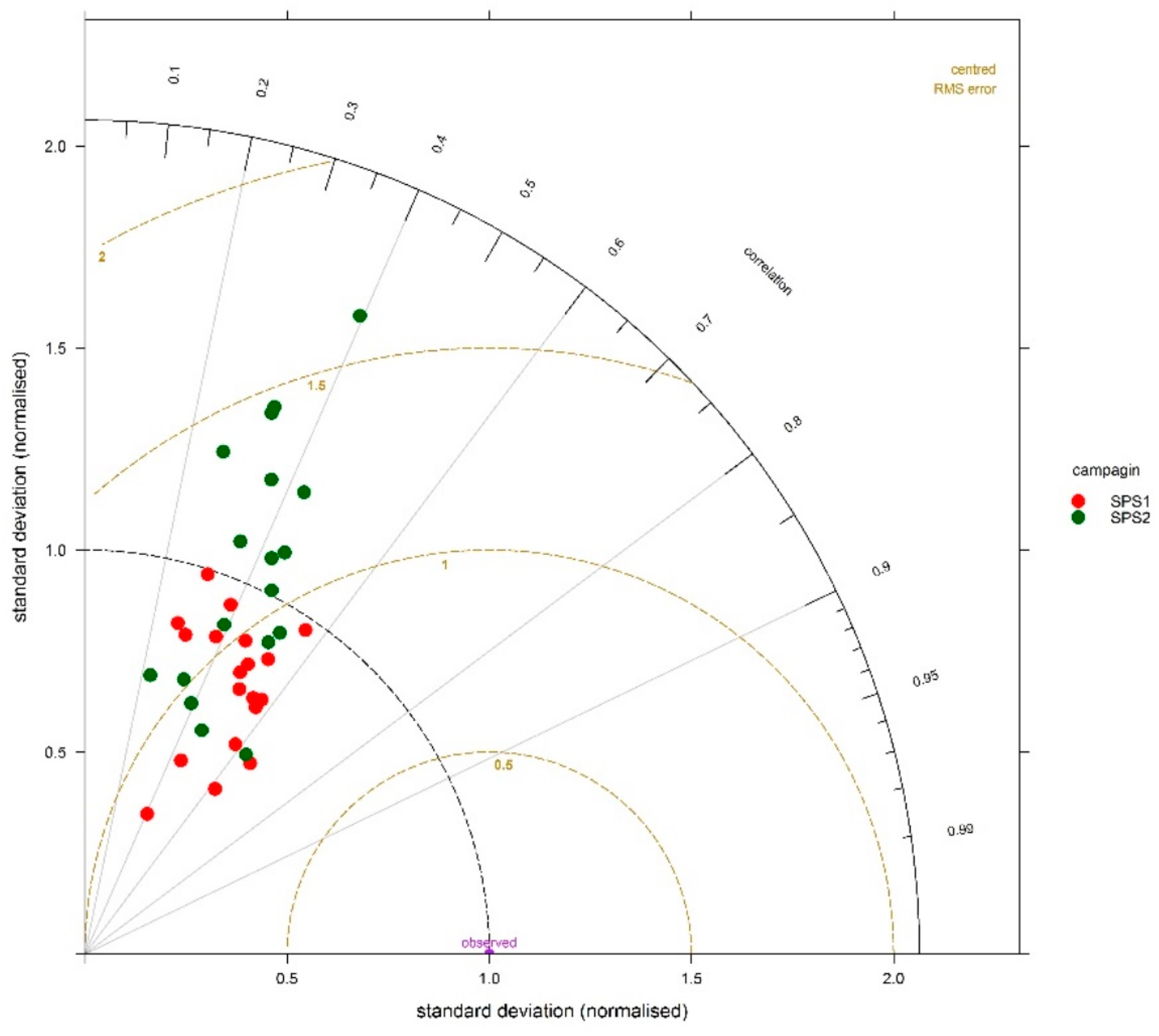
Comparisons of predicted and observed NO2 were further examined using Taylor diagram, as presented in Figure 12. For all sites in both periods, the correlations fall within a range of 0.2–0.6. The higher correlations along with lower normalized standard deviation and lower centred RMSE indicates that CCAM-CTM tends to predict NO2 in the summer months (SPS1) better than in the autumn months (SPS2).
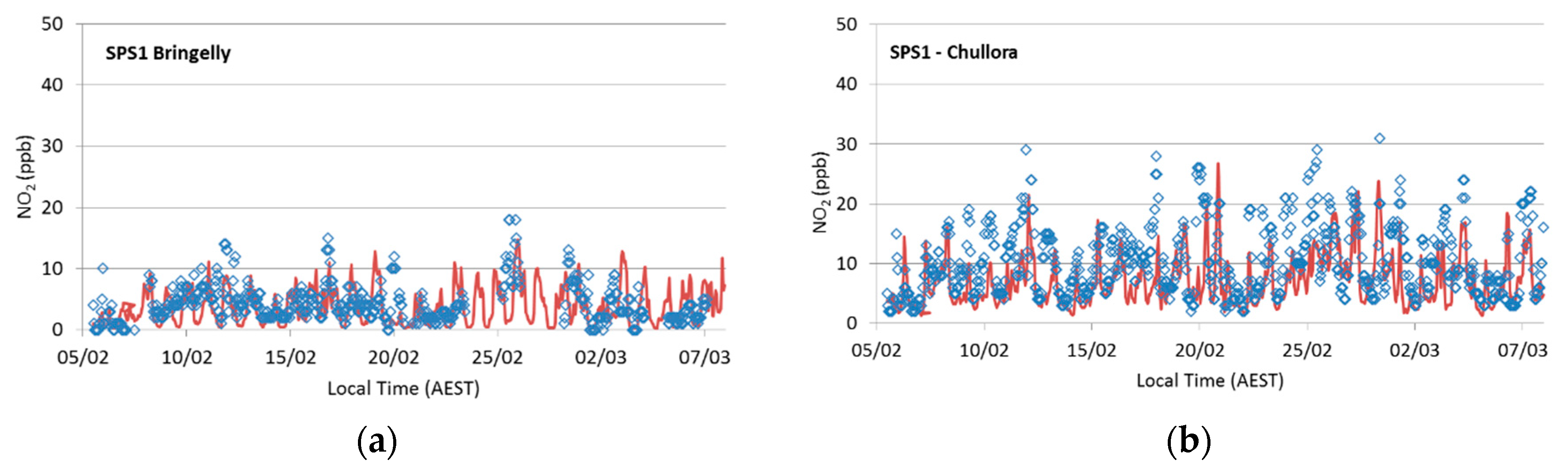
Figure 13 shows a time series of predicted and observed hourly NO2 at selected OEH sites, which represent different regions. The model generally captures the diurnal variations and magnitudes well at most sites most of time, with a tendency to underestimate NO2 across all regions. However, the model tends to overpredict NO2 peaks at Bringelly (Sydney SW region), Chullora and Randwick (Sydney East region) during SPS2 (Figure 13g–i) and underpredict NO2 peaks at Richmond (Sydney NW region), Wollongong (Illawarra region) and Newcastle (Newcastle region) (Figure 13j–l). The inaccuracies in the model NO2 predictions are assumed to be highly associated with the uncertainly in the NO2 emission estimations, the main contributions being from on-road motor vehicles and industrial sources in the NSW GMR [21].
The spatial distribution of predicted hourly average NO2 concentrations in SPS1 and SPS2 periods are shown in Figure 14. Significant elevated NO2 concentrations are found over the populated Sydney East region as well as in the Upper Hunter during both periods. The model results also show higher NO2 concentrations predicted in the autumn months in SPS2 (Figure 14b). These spatial distributions are consistent with those seen in the Ozone Monitoring Instrument (OMI) satellite observations of tropospheric NO2 columns during the periods of SPS1 and SPS2, as shown in Figure 15.

4.4. PM2.5 Components

During the Sydney Particle Study, 60 samples were collected for the measurement of aerosol chemical composition, 30 of these in the mornings and 30 samples in the afternoons [11]. This number of samples is too limited to support detailed performance statistics. Instead, model results for these periods were extracted and averaged over the full sampling season for comparison with the coinciding measurements, with a focus on the summer campaign (SPS1). Model performance is considered reasonable for modelled averages that are within a factor of two of the measured averages. The summer observation campaign identified sea salt (sodium, chloride and magnesium as marker species) and primary and secondary organic matter (organic carbon) as being the major components of PM2.5, with secondary inorganic aerosol (sulphate, ammonium, and nitrate), soil and elemental carbon also present in significant amounts.
The contribution of modelled and observed PM2.5 components are shown in Figure 16 and concentrations provided in Table 5. Only measured components of PM2.5 that correspond to modelled species are shown. The model does not explicitly predict concentrations of all measured species, accounting for several species as lumped species (e.g., dust). The components shown are sodium, chloride and magnesium (all components of sea salt), ammonium, sulphate, nitrate, elemental carbon and organic matter.
Organic matter, sodium and the secondary inorganic nitrate and sulphate components are reasonably predicted. Elemental carbon, magnesium, chloride and ammonium are underpredicted, with the predicted mass approximating only about a third of the observed mass in most cases and less than this in the case of ammonium. Results indicate that that the model underestimates the fractional sea salt contribution, and that sources of elemental carbon and ammonia are not fully accounted for in the model.

5. Conclusions

Performance evaluation and benchmarking of the coupled CCAM-CTM modelling system for the NSW GMR was conducted based on modelling results for two periods coinciding with measurement campaigns undertaken during the Sydney Particle Study. Model predictions of PM2.5, O3 and NO2 were evaluated against air quality data from the NSW OEH air quality monitoring network. The main findings of this evaluation study are summarized in the following.
  • The model generally slightly overpredicts PM2.5 with NMB less than 20%, however, moderate underpredictions of the daily peak are found on high PM2.5 days. The PM2.5 predictions at all sites comply with the performance criteria for MFB (±60%) for both periods; predictions at Earlwood and Wollongong in the summer months (SPS1), as well as Chullora, Earlwood, Richmond and Liverpool in the autumn months (SPS2) further comply with the performance goal for MFB (±30%).
  • In terms of O3, the model generally captures the diurnal variations with a slight underestimation. The model reproduces most of the high ozone events in SPS1 and captures the diurnal concentration variation in SPS2. However, the model tends to underpredict daily maximum hourly ozone. O3 predictions across all regions in SPS1, as well as in Sydney East, Sydney Northwest and Illawarra regions in SPS2, comply with the benchmark of MFB (±15%); however, none of the regions comply with the benchmark for MFE (35%).
  • For NO2, the model reproduces the diurnal variations well, with a tendency for underestimation across all regions. A better correlation between NO2 predictions and observations is found across Sydney East, Sydney Southwest, Newcastle and Illawarra regions, while poorer correlations are found for the Sydney Northwest region. Although no benchmarks were identified from the literature for NO2 validation, the MFE and NME for NO2 predictions fall within the ranges inferred from other studies.
  • For PM2.5 species, model results are within a factor of two of measured averages for sulphate, nitrate, sodium and organic matter, with underpredictions of elemental carbon, chloride, magnesium and ammonium. Results indicate the model underestimates the sea salt contribution, and that sources of elemental carbon and ammonia are not fully accounted.
The overall performance of the CCAM-CTM modelling system for the NSW GMR is comparable to similar model predictions by other regional airshed modelling documented in the literature, although the performance characteristics are found to be variable according to criteria chosen and to depend on the location of the sites, as well as the time of the year. Reasons for these discrepancies have not been clearly identified yet, due to the limitations in the operational model performance evaluation approach described in [13]. The detailed statistics reported in this study not only benchmark the overall model performance, but also identify several areas of potential improvements for CCAM-CTM modelling in the future including: (1) a better capture of highly variable emissions, in terms of magnitude and spatial distributions for sources such as motor vehicles, residential wood heaters and industrial sources; (2) a “diagnostic” evaluation to characterise the response of regional elevated ozone concentrations to changes in NOx and VOC emissions; and (3) a sensitivity analysis with various surface roughness scheme to understand the CCAM wind predictions. Based on this benchmarking exercise, the application of the CCAM-CTM modelling system for the NSW GMR to assist air policy development and air quality management in NSW is supported.

Author Contributions

Conceptualization, L.T.-C.C. and Y.S.; Data curation, T.T.; Formal analysis, L.T.-C.C.; Investigation, L.T.-C.C.; Methodology, H.N.D., K.M. and N.J.; Resources, Y.S.; Software, H.N.D., T.T. and K.M.; Writing—original draft, L.T.-C.C.; and Writing—review and editing, H.N.D., Y.S., K.M. and N.J.

Funding

This research received no external funding.

Acknowledgments

The authors gratefully acknowledge discussions with Martin Cope (CSIRO), Yang Zhang (North Carolina State University), and Elise-Andree Guérette, Jeremy Silver and Steven Utembe in the Clean Air and Urban Landscapes Hub (CAUL). We acknowledge that the visualizations of satellite data were produced with the Giovanni online data system, developed and maintained by the NASA GES DISC. We also acknowledge the helpful comments from the referees that improved this manuscript.

Conflicts of Interest

The authors declare no conflicts of interest.

Appendix A

Table A1. The source-dependent fractions for major source groups used in emission modelling.
Major Source GroupsPM2.5/PM10EC/PM10OC/PM10DU/PM10LEVO/PM10SO3/PM10SO3/SOxIOLE/OLEALDX/ALD2ETHA/PARPTOL/TOLPXYL/XYLPBNZ/TOL
Petrol exhaust0.9700.3290.4010.2700.00.02850.030.3740.1450.00.770.480.31
Diesel exhaust0.9530.2830.6350.0830.00.0440.030.1850.340.0850.770.480.31
Other exhaust0.9530.2830.6350.0830.0−1.00.030.4910.6500.1230.770.480.31
Petrol evaporation0.9530.2830.6350.0830.0−1.00.030.4910.6500.1230.770.480.31
Shipping and commercial boats0.9700.0080.1910.1560.00.6450.000.00.00.00.770.480.31
Industrial vehicles and equipment0.9700.6430.2370.1200.0−1.00.030.00.00.00.770.480.31
Aircraft0.8440.760.240.00.0−1.00.030.00.00.00.770.480.31
Locomotives0.9700.7710.1760.0530.0−1.00.030.00.00.00.770.480.31
Commercial non-road equipment0.9700.6430.2370.1200.0−1.00.030.00.00.00.770.480.31
Non-exhaust particulate matter0.5320.010.0940.8930.00.01350.000.00.00.00.00.00.0
Residential Woodheaters0.9630.1510.4190.4310.25−1.00.030.00.00.00.770.480.31
Industrial area fugitives0.1700.0050.10.90.00.0010.000.00.00.00.00.00.0
Other domestic-commercial area source (excluding non-road and wood heaters)0.3000.1000.1000.8000.0−1.00.030.00.00.00.770.480.31
EC, elemental carbon; OC, organic carbon; DU, dust; LEVO, levoglucosan; OLE, olefins; IOLE, internal olefin species; ALD2, acetaldehyde, ALDX, all other higher aldehydes; PAR, paraffins; ETHA, ethane; TOL, toluene; PTOL, primary-toluene; XYL, xylene; PXYL, primary-xylene; PBNZ, primary-benzene.

Appendix B

Table A2. Quantitative statistical model performance metrics.
MetricsMathematical ExpressionRange
Mean Bias (MB) MB = 1 n i = 1 n ( M i O i ) −∞ to +∞
Mean Error (ME) ME = 1 n i = 1 n | M i O i | 0 to +∞
Normalized Mean Bias (NMB) NMB = 1 n i = 1 n ( M i O i ) O i −100% to +∞
Normalized Mean Error (NME) NME = 1 n i = 1 n | M i O i | O i 0% to +∞
Mean Fractional Bias (MFB) MFB = 1 n i = 1 n ( M i O i ) ( M i + O i ) 2 −200% to 200%
Mean Fractional Error (MFE) MFE = 1 n i = 1 n | M i O i | ( M i + O i ) 2 0% to 200%
Root Mean Square Error (RMSE) RMSE = 1 n i = 1 n ( M i O i ) 2 0 to +∞
Correlation coefficient (R) R =   i = 1 n ( ( O i O ¯ ) ( M i M ¯ ) ) i = 1 n ( O i O ¯ ) 2 i = 1 n ( M i M ¯ ) 2 −1 to 1
Index of Agreement (IOA) IOA = 1   i = 1 n ( M i O i ) 2 i = 1 n ( | M i O ¯ | + | O i O ¯ | ) 2 0 to 1

Appendix C

Table A3. Quantitative performance statistics for predicted hourly (a) NO, (b) CO and (c) SO2 concentrations against observations in the Sydney East, Sydney NW, Sydney SW, Illawarra and Newcastle regions for the periods of SPS1 and SPS2. Table (a) illustrates the CCAM-CTM has a tendency to underpredict hourly NO concentrations with values of MB (ME) in a range of −1.79 to −6.31 ppb (4.15 to 7.07 ppb) in SPS1 and −3.03 to −17.15 ppb (9.9 to 18.34 ppb) in SPS2 across regions. The model generally performs better in predicting NO in the Sydney East and Sydney SW regions, in terms of higher values of correlation coefficient and IOA are found in both regions during SPS1 and SPS2, while the lowest values of correlation coefficient and IOA are found in the Illawarra region in both periods. The CCAM-CTM shows a larger tendency to underpredict hourly CO concentrations with values of MB (ME) vary from −40.37 to −233.74 ppb (48.67 to 251.71 ppb) during SPS1 and SPS2. Relatively higher values of correlation coefficient (0.42 to 0.45) and IOA (0.64 to 0.73) are found in the Sydney East region in both SPS1 and SPS2. Quantitative performance statistics for predicted hourly SO2 concentrations are summarised in Table (c). The model generally overpredict SO2 with values of MB (ME) in a range of 0.36 to 0.89 ppb (0.83 to 2.25 ppb) in both periods. Higher values of IOA are found in the Sydney NW and SW regions (0.81 to 0.9), while higher values of correlation coefficient (0.57) was found in Newcastle.
(a)
NOSPS1SPS2
Sydney EastSydney NWSydney SWIllawarraNewcastleSydney EastSydney NWSydney SWIllawarraNewcastle
Mean CTM (ppb)5.952.732.262.101.1516.248.456.032.381.87
Std (ppb)8.802.762.501.331.1424.0810.428.361.882.44
Mean Obs (ppb)7.745.388.564.775.0819.2612.1913.8910.7319.02
Std (ppb)12.538.2312.167.408.5226.0715.6518.5718.1827.46
MB (ppb)−1.79−2.65−6.31−3.45−3.93−3.03−3.75−7.86−8.35−17.15
NMB−19%−4%−157%−69%−82%−11%−43%−49%−77%−90%
MFB−16%−46%−96%−85%−88%−17%−64%−96%−59%−123%
ME (ppb)6.374.407.074.164.1518.3412.4012.009.9017.48
NME51%60%71%67%49%76%81%69%52%64%
MFE82%92%112%112%98%96%113%122%106%134%
RMSE (ppb)7.762.592.311.301.0723.2211.107.812.362.44
Corr. Coeff.0.470.160.210.180.350.240.110.33−0.050.06
IOA0.710.780.800.650.710.510.640.730.560.55
(b)
COSPS1SPS2
Sydney EastSydney NWSydney SWIllawarraNewcastleSydney EastSydney NWSydney SWIllawarraNewcastle
Mean CTM (ppb)120.67102.8799.46245.7485.05211.71203.03146.54N/A98.52
Std (ppb)76.6839.5363.65240.2523.63153.22147.54119.48 30.65
Mean Obs (ppb)325.70315.84323.50343.45125.42445.45395.13343.69 244.59
Std (ppb)134.78111.14107.57176.0064.47291.23236.36207.73 264.11
MB (ppb)−205.03−212.97−224.04−97.70−40.37−233.74−192.09−197.15 −146.07
NMB−63%−67%−69%−28%−33%−52%−49%−57% −79%
MFB−93%−102%−107%−61%−34%−70%−63%−81% −55%
ME (ppb)209.23213.65227.82276.0548.67251.71223.42209.58 154.20
NME156%192%217%157%76%86%95%108% 58%
MFE95%102%109%95%41%76%72%84% 62%
RMSE (ppb)77.3251.0064.76298.5523.11136.88141.37107.40 29.79
Corr. Coeff.0.420.370.160.060.210.450.290.43 0.24
IOA0.730.720.740.690.730.640.630.68 0.37
(c)
SO2SPS1SPS2
Sydney EastSydney NWSydney SWIllawarraNewcastleSydney EastSydney NWSydney SWIllawarraNewcastle
Mean CTM (ppb)2.392.091.703.963.192.852.141.541.143.62
Std (ppb)0.930.800.661.681.641.000.620.761.981.99
Mean Obs (ppb)1.811.571.343.152.791.961.391.191.762.99
Std (ppb)1.491.200.793.262.552.000.750.431.553.08
MB (ppb)0.580.520.360.810.400.890.750.36−0.620.63
NMB31%36%30%17%15%45%55%−21%−31%21%
MFB−48%−56%−47%−13%−20%−70%−87%−71%−3%−19%
ME (ppb)1.241.100.832.251.601.430.940.901.832.12
NME93%95%112%73%63%73%126%263%117%69%
MFE80%86%77%71%66%95%99%96%83%75%
RMSE (ppb)0.970.810.611.501.350.990.610.701.901.90
Corr. Coeff.0.130.140.210.140.570.180.210.170.280.30
IOA0.760.820.900.790.900.730.810.880.670.66

References

  1. Thunis, P.; Miranda, A.; Baldasano, J.M.; Blond, N.; Douros, J.; Graff, A.; Janssen, S.; Juda-Rezler, K.; Karvosenoja, N.; Maffeis, G.; et al. Overview of Current Regional and Local Scale Air Quality Modelling Practices: Assessment and Planning Tools in the EU. Environ. Sci. Policy 2016, 65, 13–21. [Google Scholar] [CrossRef]
  2. Saikawa, E.; Kurokawa, J.; Takigawa, M.; Borken-Kleefeld, J.; Mauzerall, D.L.; Horowitz, L.W.; Ohara, T. The Impact of China’s Vehicle Emissions on Regional Air Quality in 2000 and 2020: A Scenario Analysis. Atmos. Chem. Phys. 2011, 11, 9465–9484. [Google Scholar] [CrossRef]
  3. Frost, G.J.; McKeen, S.A.; Trainer, M.; Ryerson, T.B.; Neuman, J.A.; Roberts, J.M.; Swanson, A.; Holloway, J.S.; Sueper, D.T.; Fortin, T.; et al. Effects of Changing Power Plant Nox Emissions on Ozone in the Eastern United States: Proof of Concept. J. Geophys. Res. Atmos. 2006, 111. [Google Scholar] [CrossRef]
  4. Chemel, C.; Fisher, B.E.A.; Kong, X.; Francis, X.V.; Sokhi, R.S.; Good, N.; Collins, W.J.; Folberth, G.A. Application of Chemical Transport Model CMAQ to Policy Decisions Regarding PM2.5 in the UK. Atmos. Environ. 2014, 82, 410–417. [Google Scholar] [CrossRef]
  5. Wang, Z.; Pan, L.; Li, Y.; Zhang, D.; Ma, J.; Sun, F.; Xu, W.; Wang, X. Assessment of Air Quality Benefits from the National Pollution Control Policy of Thermal Power Plants in China: A Numerical Simulation. Atmos. Environ. 2015, 106, 288–304. [Google Scholar] [CrossRef]
  6. Kukkonen, J.; Olsson, T.; Schultz, D.M.; Baklanov, A.; Klein, T.; Miranda, A.I.; Monteiro, A.; Hirtl, M.; Tarvainen, V.; Boy, M.; et al. A Review of Operational, Regional-Scale, Chemical Weather Forecasting Models in Europe. Atmos. Chem. Phys. 2012, 12, 1–87. [Google Scholar] [CrossRef]
  7. Cope, M.E.; Hess, G.D.; Lee, S.; Tory, K.; Azzi, M.; Carras, J.; Lilley, W.; Manins, P.C.; Nelson, P.; Ng, L.; et al. The Australian Air Quality Forecasting System. Part I: Project Description and Early Outcomes. J. Appl. Meteorol. 2004, 43, 649–662. [Google Scholar] [CrossRef]
  8. Hu, J.; Zhang, H.; Ying, Q.; Chen, S.H.; Vandenberghe, F.; Kleeman, M.J. Long-Term Particulate Matter Modeling for Health Effect Studies in California—Part 1: Model Performance on Temporal and Spatial Variations. Atmos. Chem. Phys. 2015, 15, 3445–3461. [Google Scholar] [CrossRef]
  9. Buonocore, J.J.; Dong, X.; Spengler, J.D.; Fu, J.S.; Levy, J.I. Using the Community Multiscale Air Quality (Cmaq) Model to Estimate Public Health Impacts of PM2.5 from Individual Power Plants. Environ. Int. 2014, 68, 200–208. [Google Scholar] [CrossRef]
  10. Cope, M.; Lee, S.; Noonan, J.; Lilley, B.; Hess, D.; Azzi, M. Chemical Transport Model—Technical Description; CSIRO: Canberra, Australia, 2009; p. 114. [Google Scholar]
  11. Cope, M.; Keywood, M.; Emmerson, K.; Galbally, I.; Boast, K.; Chambers, S.; Cheng, M.; Crumeyrolle, S.; Dunne, E.; Fedele, R.; et al. Sydney Particle Study; CSIRO: Canberra, Australia, 2014; p. 151. [Google Scholar]
  12. US-EPA. Guidance on the Use of Models and Other Analyses for Demonstrating Attainment of Air Quality Goals for Ozone, PM2.5, and Regional Haze; US-EPA: Washington, DC, USA, 2007; p. 253.
  13. Dennis, R.; Fox, T.; Fuentes, M.; Gilliland, A.; Hanna, S.; Hogrefe, C.; Irwin, J.; Rao, S.T.; Scheffe, R.; Schere, K.; et al. A Framework for Evaluating Regional-Scale Numerical Photochemical Modeling Systems. Environ. Fluid Mech. 2010, 10, 471–489. [Google Scholar] [CrossRef]
  14. Derwent, D.; Fraser, A.; Abbott, J.; Jenkin, M.; Willis, P.; Murrells, T. Evaluating the Performance of Air Quality Models; UK Department for Environment, Food and Rural Affairs: London, UK, 2010; p. 73.
  15. EEA. The Application of Models under the European Union’s Air Quality Directive: A Technical Reference Guide; European Environment Agency: København, Denmark, 2011. [Google Scholar]
  16. Thunis, P.; Georgieva, E.; Pederzoli, A. A Tool to Evaluate Air Quality Model Performances in Regulatory Applications. Environ. Model. Softw. 2012, 38, 220–230. [Google Scholar] [CrossRef]
  17. Rao, S.T.; Galmarini, S.; Puckett, K. Air Quality Model Evaluation International Initiative (AQMEII): Advancing the State of the Science in Regional Photochemical Modeling and Its Applications. Bull. Am. Meteorol. Soc. 2010, 92, 23–30. [Google Scholar] [CrossRef]
  18. Appel, K.W.; Chemel, C.; Roselle, S.J.; Francis, X.V.; Hu, R.-M.; Sokhi, R.S.; Rao, S.T.; Galmarini, S. Examination of the Community Multiscale Air Quality (CMAQ) Model Performance over the North American and European Domains. Atmos. Environ. 2012, 53, 142–155. [Google Scholar] [CrossRef]
  19. McGregor, J.L.; Dix, M.R. An Updated Description of the Conformal-Cubic Atmospheric Model. In High Resolution Numerical Modelling of the Atmosphere and Ocean; Springer: New York, NY, USA, 2008; pp. 51–75. [Google Scholar]
  20. McGregor, J.L. C-Cam Geometric Aspects and Dynamical Formulation; CSIRO: Canberra, Australia, 2005; p. 43. [Google Scholar]
  21. NSW-EPA. 2008 Calendar Year Air Emissions Inventory for the Greater Metropolitan Region in Nsw; NSW-EPA: Sydney, Australia, 2012.
  22. Hurley, P. Tapm V4. Part 1: Technical Description; CSIRO: Canberra, Australia, 2008. [Google Scholar]
  23. Galbally, I.; Cope, M.; Lawson, S.; Bentley, S.; Cheng, M.; Gillett, R.; Selleck, P.; Petraitis, B.; Dunne, E.; Lee, S. Sources of Ozone Precursors and Atmospheric Chemistry in a Typical Australian City; Dept. of the Environment and Water Resources: Canberra, Australia, 2009. [Google Scholar]
  24. Sarwar, G.; Luecken, D.; Yarwood, G.; Whitten, G.Z.; Carter, W.P.L. Impact of an Updated Carbon Bond Mechanism on Predictions from the CMAQ Modeling System: Preliminary Assessment. J. Appl. Meteorol. Clim. 2008, 47, 3–14. [Google Scholar] [CrossRef]
  25. Sarwar, G.; Appel, K.W.; Carlton, A.G.; Mathur, R.; Schere, K.; Zhang, R.; Majeed, M.A. Impact of a New Condensed Toluene Mechanism on Air Quality Model Predictions in the Us. Geosci. Model Dev. 2011, 4, 183–193. [Google Scholar] [CrossRef]
  26. Fountoukis, C.; Nenes, A. Isorropia II: A Computationally Efficient Thermodynamic Equilibrium Model for K+–Ca2+–Mg2+–Nh4+–Na+–SO42−–NO3–Cl–H2O Aerosols. Atmos. Chem. Phys. 2007, 7, 4639–4659. [Google Scholar] [CrossRef]
  27. Donahue, N.M.; Robinson, A.L.; Stanier, C.O.; Pandis, S.N. Coupled Partitioning, Dilution, and Chemical Aging of Semivolatile Organics. Environ. Sci. Technol. 2006, 40, 2635–2643. [Google Scholar] [CrossRef]
  28. Mann, G.W.; Carslaw, K.S.; Spracklen, D.V.; Ridley, D.A.; Manktelow, P.T.; Chipperfield, M.P.; Pickering, S.J.; Johnson, C.E. Description and Evaluation of Glomap-Mode: A Modal Global Aerosol Microphysics Model for the Ukca Composition-Climate Model. Geosci. Model Dev. 2010, 3, 519–551. [Google Scholar] [CrossRef]
  29. Zhang, R.; Wang, Z.; Shen, Z.; Yabuki, S.; Kanai, Y.; Ohta, A. Physicochemical Characterization and Origin of the 20 March 2002 Heavy Dust Storm in Beijing. Aerosol Air Qual. Res. 2006, 6. [Google Scholar] [CrossRef]
  30. Boylan, J.W.; Russell, A.G. PM and Light Extinction Model Performance Metrics, Goals, and Criteria for Three-Dimensional Air Quality Models. Atmos. Environ. 2006, 40, 4946–4959. [Google Scholar] [CrossRef]
  31. Monk, K.; Guérette, E.-A.; Paton-Walsh, C.; Silver, J.D.; Emmerson, K.; Utembe, S.; Zhang, Y.; Griffiths, A.; Chang, L.T.-C.; Duc, H.; et al. Evaluation of Regional Air Quality Models over Sydney, Australia: Part 1 Meteorological Model Comparison. Atmosphere 2018, 9. under review. [Google Scholar]
  32. Chemel, C.; Sokhi, R.S.; Yu, Y.; Hayman, G.D.; Vincent, K.J.; Dore, A.J.; Tang, Y.S.; Prain, H.D.; Fisher, B.E.A. Evaluation of a CMAQ Simulation at High Resolution over the UK for the Calendar Year 2003. Atmos. Environ. 2010, 44, 2927–2939. [Google Scholar] [CrossRef]
  33. Cohen, D.D.; Atanacio, A.J.; Stelcer, E.; Garton, D. Sydney Particle Characterisation Study; Australian Nuclear Science and Technology Organisation: Lucas Heights, Australia, 2016; p. 156.
  34. Simon, H.; Baker, K.R.; Phillips, S. Compilation and Interpretation of Photochemical Model Performance Statistics Published between 2006 and 2012. Atmos. Environ. 2012, 61, 124–139. [Google Scholar] [CrossRef]
  35. Hibberd, M.; Selleck, P.; Keywood, M.; Cohen, D.; Stelcer, E.; Atanacio, A. Upper Hunter Valley Particle Characterization Study; CSIRO: Canberra, Australia, 2013; p. 72. [Google Scholar]
  36. Zhang, Y.; Liu, P.; Queen, A.; Misenis, C.; Pun, B.; Seigneur, C.; Wu, S.-Y. A Comprehensive Performance Evaluation of MM5-CMAQ for the Summer 1999 Southern Oxidants Study Episode—Part II: Gas and Aerosol Predictions. Atmos. Environ. 2006, 40, 4839–4855. [Google Scholar] [CrossRef]
  37. Duc, H.; Azzi, M.; Wahid, H.; Ha, Q.P. Background Ozone Level in the Sydney Basin: Assessment and Trend Analysis. Int. J. Clim. 2013, 33, 2298–2308. [Google Scholar] [CrossRef]
  38. Yu, Y.; Sokhi, R.S.; Kitwiroon, N.; Middleton, D.R.; Fisher, B. Performance Characteristics of MM5–Smoke–CMAQ for a Summer Photochemical Episode in Southeast England, United Kingdom. Atmos. Environ. 2008, 42, 4870–4883. [Google Scholar] [CrossRef]
  39. Gao, Y.; Fu, J.S.; Drake, J.B.; Lamarque, J.F.; Liu, Y. The Impact of Emission and Climate Change on Ozone in the United States under Representative Concentration Pathways (RCPs). Atmos. Chem. Phys. 2013, 13, 9607–9621. [Google Scholar] [CrossRef]
  40. Acker, J.G.; Leptoukh, G. Online Analysis Enhances Use of NASA Earth Science Data. EOS Trans. Am. Geophys. Union 2007, 88, 14–17. [Google Scholar] [CrossRef]
Figure 1. Schematic diagram of the CCAM-CTM modelling system.
Atmosphere 09 00486 g001
Figure 2. Domain configuration of the CCAM-CTM modelling system. The four nested domains are with a horizontal resolution of 80-km (AUS), 27-km (NSW), 9-km (GMR) and 3-km (SYD), respectively.
Atmosphere 09 00486 g002
Figure 3. Total emissions (tons/year) of: (a) PM10; (b) PM2.5; (c) NOx; (d) VOCs; (e) SO2; and (f) NH3 from the 2008 NSW GMR emission inventory.
Atmosphere 09 00486 g003
Figure 4. Location of 18 OEH air quality monitoring stations (yellow dots) and six BOM weather stations (blue dots) used for model performance evaluation. All stations are within the innermost Sydney domain (SYD) used for CCAM-CTM simulation with a horizontal resolution of 3 km with two exceptions of OEH Newcastle station and BOM Williamtown RAAF.
Atmosphere 09 00486 g004
Figure 5. Bugle plots of (a) mean fractional bias (MFB) and (b) mean fractional error (MFE) for PM2.5 for all predicted/observed pairs values at Chullora, Earlwood, Richmond, Liverpool and Wollongong stations for SPS1 (black star) and SPS2 (green triangle).
Atmosphere 09 00486 g005
Figure 6. Taylor diagram of hourly PM2.5 for all predicted/observed pairs of values at Chullora, Earlwood, Richmond, Liverpool and Wollongong stations for SPS1 (red dot) and SPS2 (green dot).
Atmosphere 09 00486 g006
Figure 7. The time series of predicted (red line) and observed (blue hollow dot) hourly PM2.5 concentrations (µg/m3) at Chullora, Earlwood, Richmond, Liverpool and Wollongong stations for: SPS1 (ae); and SPS2 (fj).
Atmosphere 09 00486 g007aAtmosphere 09 00486 g007b
Figure 8. Spatial distribution of PM2.5 concentrations (µg/m3) predicted by CCAM-CTM with GMR 9-km horizontal resolution domain. The hourly average PM2.5 concentrations for the period of (a) SPS1 and (b) SPS2; and the hourly maximum PM2.5 concentrations for the period of (c) SPS1 and (d) SPS2. Red cross signs indicate locations of OEH stations where PM2.5 measurements are available.
Atmosphere 09 00486 g008aAtmosphere 09 00486 g008b
Figure 9. Tayler diagram of hourly O3 for all predicted/observed pairs of values at 18 OEH stations for SPS1 (red dot) and SPS2 (green dot).
Atmosphere 09 00486 g009
Figure 10. The time series of predicted (red line) and observed (blue hollow dot) hourly O3 (ppb) at selected six OEH stations during: SPS1 (af); and SPS2 (gl).
Atmosphere 09 00486 g010aAtmosphere 09 00486 g010b
Figure 11. Spatial distribution of O3 concentrations (ppb) predicted by CCAM-CTM with GMR 9-km horizontal resolution domain. The hourly average O3 concentrations for the period of (a) SPS1 and (b) SPS2; and the average of O3 daily maximums for the period of (c) SPS1 and (d) SPS2. Red cross signs indicate locations of OEH stations.
Atmosphere 09 00486 g011aAtmosphere 09 00486 g011b
Figure 12. Tayler diagram of hourly NO2 for all predicted/observed pairs of values at 18 OEH stations for SPS1 (red dot) and SPS2 (green dot).
Atmosphere 09 00486 g012
Figure 13. The time series of predicted (red line) and observed (blue hollow dot) hourly NO2 (ppb) at selected 6 OEH stations during: SPS1 (af); and SPS2 (gl).
Atmosphere 09 00486 g013aAtmosphere 09 00486 g013b
Figure 14. Spatial distribution of NO2 concentrations (ppb) predicted by CCAM-CTM with GMR 9-km horizontal resolution domain. The hourly average NO2 concentrations for the period of: (a) SPS1; and (b) SPS2. Red cross signs indicate locations of OEH stations.
Atmosphere 09 00486 g014
Figure 15. Time averaged map of NO2 tropospheric column (30% cloud screened) daily 0.25° (OMI OMNO2d v003) 1/cm2 over the periods of: (a) SPS1; and (b) SPS2. Analysed by NASA Giovanni platform [40].
Atmosphere 09 00486 g015
Figure 16. Modelled and observed average concentrations of PM2.5 species at Westmead for SPS1.
Atmosphere 09 00486 g016
Table 1. The 16 major source groups segregated from the 2008 NSW GMR emission inventory.
CategoryMajor Source Group
On-road motor vehiclesPetrol exhaust
Diesel exhaust
Other exhaust
Petrol evaporation
Non-exhaust particulate matter
Non-road diesel and marineShipping and commercial boats
Industrial vehicles and equipment
Aircraft (flight and ground operations)
Locomotives
Commercial non-road equipment
Industrial point sourcesPower generation from coal
Power generation from gas
Other industrial point sources
Other industrial, commercial and domestic-commercial area sourcesResidential wood heating
Industrial area fugitive emissions
Other domestic-commercial area source emissions (non-road diesel and marine sources and wood heating are excluded)
Table 2. Quantitative performance statistics for predicted hourly PM2.5 concentration against observations at Chullora, Earlwood, Richmond, Liverpool and Wollongong for the periods of SPS1 and SPS2.
PM2.5SPS1SPS2
ChulloraEarlwoodRichmondLiverpoolWollongongChulloraEarlwoodRichmondLiverpoolWollongong
Mean CTM (µg m−3)6.256.035.835.976.107.546.844.336.594.97
Std (µg m−3)2.942.892.722.872.833.763.472.103.662.32
Mean Obs (µg m−3)6.545.454.914.995.536.406.204.087.394.17
Std (µg m−3)4.423.653.313.604.024.864.882.896.683.14
MB (µg m−3)−0.280.580.920.980.561.140.640.25−0.800.80
NMB−4%11%19%20%10%18%10%6%−11%19%
MFB58%23%47%35%24%30%28%18%13%32%
ME (µg m−3)2.862.542.622.642.813.383.492.524.652.62
NME65%70%79%73%70%70%71%87%70%83%
MFE69%50%60%46%53%54%60%62%64%63%
RMSE (µg m−3)2.682.482.482.482.603.263.112.073.552.20
Corr. Coeff.0.410.510.410.500.390.500.440.180.240.31
IOA0.610.660.610.660.610.670.640.480.490.54
Table 3. Quantitative performance statistics for predicted hourly O3 concentration against observations in the Sydney East, Sydney NW, Sydney SW, Illawarra and Newcastle regions for the periods of SPS1 and SPS2.
O3SPS1SPS2
Sydney EastSydney NWSydney SWIllawarraNewcastleSydney EastSydney NWSydney SWIllawarraNewcastle
Mean CTM (ppb)15.4016.3716.3817.3917.789.728.4212.7010.3115.76
Std (ppb)9.8311.5810.268.428.117.458.217.695.097.21
Mean Obs (ppb)16.1817.6918.7016.8718.8011.9012.3715.7816.2312.21
Std (ppb)9.4011.6511.319.629.389.249.878.118.589.33
MB (ppb)−0.79−1.32−2.310.52−1.02−2.18−1.14−3.07−0.763.55
NMB−4%−7%−11%4%−5%−17%−9%−16%−5%29%
MFB−4%−6%−9%11%2%−19%−5%−20%9%45%
MFB _15 *−23%−26%−26%−18%−17%−48%−37%−26%−30%−9%
ME (ppb)6.036.536.686.995.576.396.046.556.986.96
NME65%56%59%73%59%69%61%92%81%75%
MFE45%48%44%45%36%72%70%59%53%67%
MFE_15 *35%38%37%33%26%53%45%53%34%27%
RMSE (ppb)7.317.647.297.176.166.236.026.014.935.88
Corr. Coeff.0.660.750.690.510.650.540.680.600.340.58
IOA0.800.870.820.640.770.760.810.780.550.68
* MFB _15 and MFE_15 are statistics calculated with implementations of cut-off concentrations of 15 ppb for background ozone.
Table 4. Quantitative performance statistics for predicted hourly NO2 concentration against observations in the Sydney East, Sydney NW, Sydney SW, Illawarra and Newcastle regions for the periods of SPS1 and SPS2.
NO2SPS1SPS2
Sydney EastSydney NWSydney SWIllawarraNewcastleSydney EastSydney NWSydney SWIllawarraNewcastle
Mean CTM (ppb)7.014.604.013.742.6012.935.626.235.115.38
Std (ppb)4.443.163.112.462.408.715.655.454.824.23
Mean Obs (ppb)8.126.105.375.544.8513.338.267.257.8411.61
Std (ppb)5.323.814.074.544.587.085.525.016.116.72
MB (ppb)−1.11−1.50−1.36−1.80−2.26−0.40−0.76−1.02−2.73−6.23
NMB−13%−25%−28%−28%−46%−1%−12%−21%−33%−54%
MFB−10%−32%−38%−28%−54%−6%−17%−40%−36%−72%
ME (ppb)4.033.012.923.872.766.634.524.274.226.63
NME76%80%75%87%60%95%85%86%68%99%
MFE55%60%72%82%68%54%64%76%62%80%
RMSE (ppb)3.872.882.682.361.937.774.674.814.073.71
Corr. Coeff.0.490.390.480.200.590.450.350.440.540.48
IOA0.710.610.700.660.680.660.620.690.720.64
Table 5. Comparison of modelled and measured average concentrations of PM2.5 speciated components measured at Westmead during SPS1.
PM2.5 ComponentWestmead
Mean CTM (µg m−3)Mean Obs (µg m−3)Ratio CTM/Obs
Nitrate0.430.650.65
Ammonium0.060.340.17
Sulphate0.881.560.56
Sodium0.661.200.55
Magnesium0.050.150.31
Chloride0.411.390.30
Elemental Carbon0.300.930.33
Organic Matter2.813.150.89

