Closing the N-Budget: How Simulated Groundwater-Borne Nitrate Supply Affects Plant Growth and Greenhouse Gas Emissions on Temperate Grassland

 , , , ,
Abstract
:
1. Introduction
2. Materials and Methods
2.1. Field Site
2.2. Data Implementation
2.3. N Balance
2.4. LandscapeDNDC: Model Setup
2.5. Sensitivity Analysis and Calibration
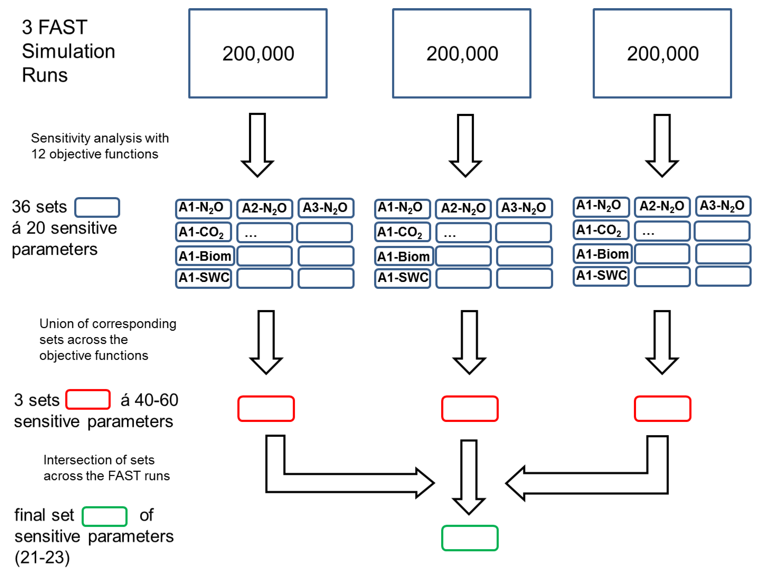
2.5.1. Sensitivity Analysis
2.5.2. Calibration
3. Results
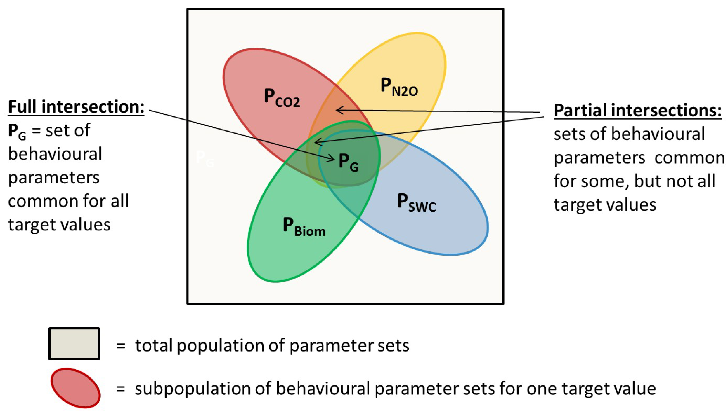
3.1. Sensitive Parameters and Intersection Sizes
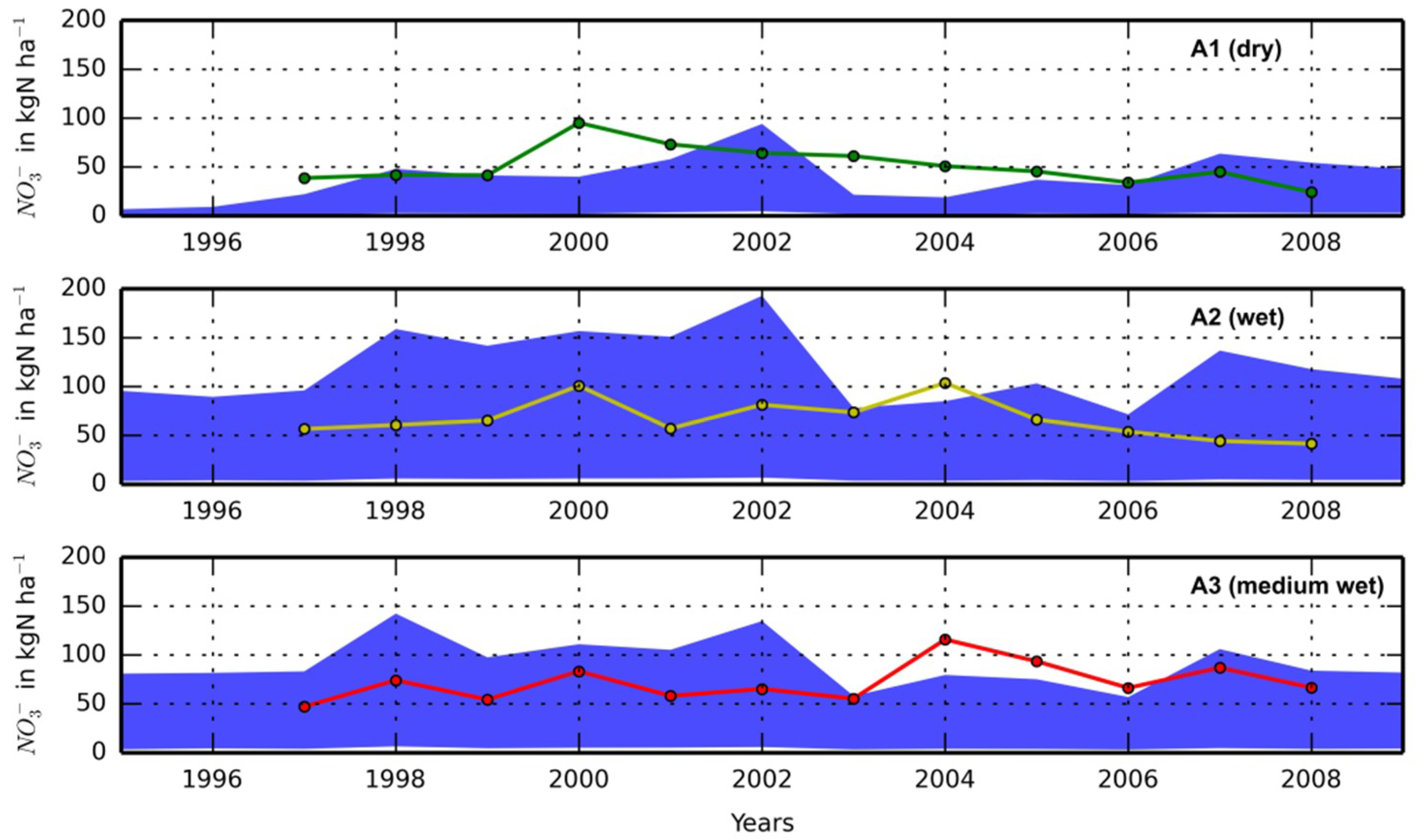
3.2. NO3− Uptake
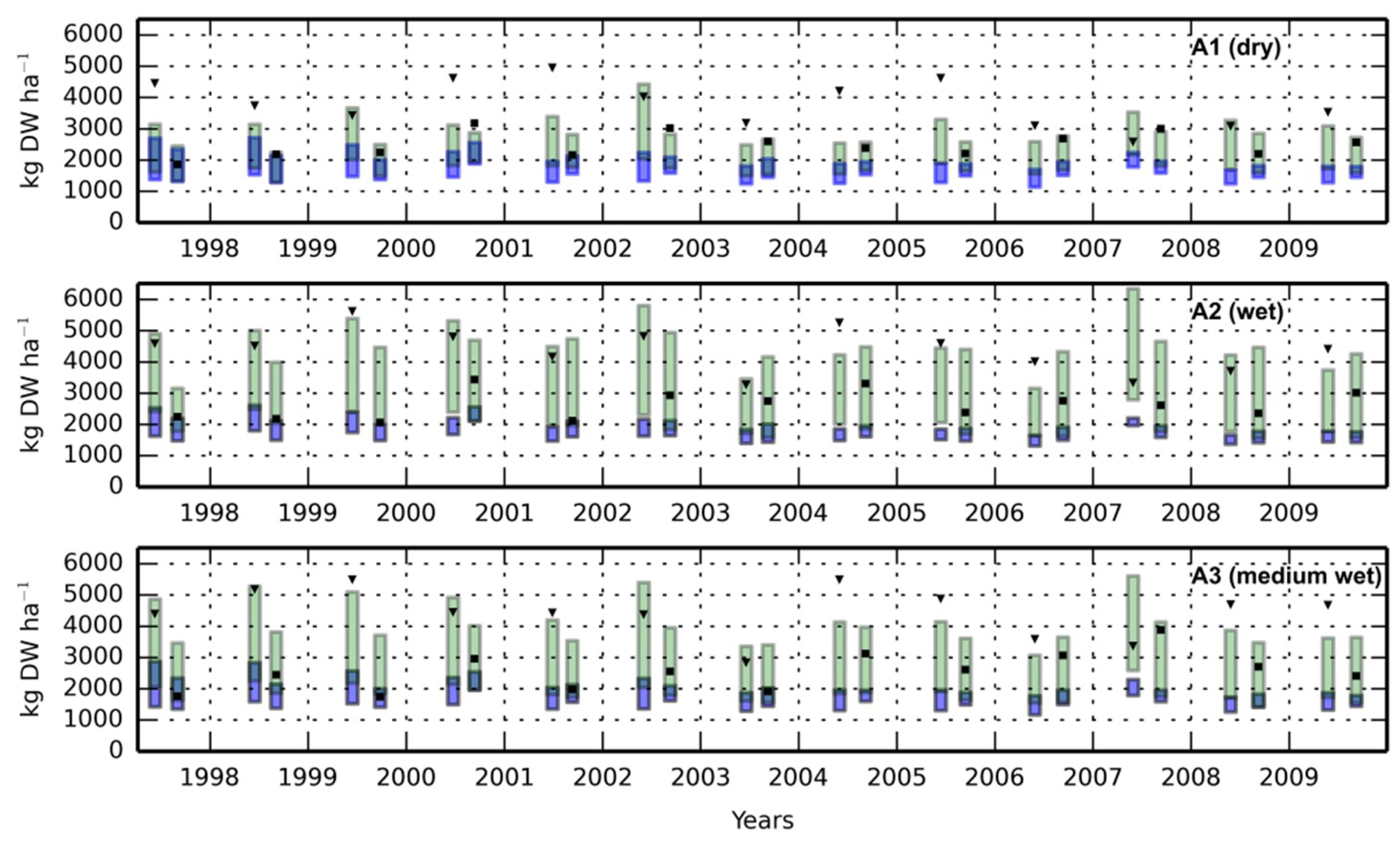
3.3. Biomass
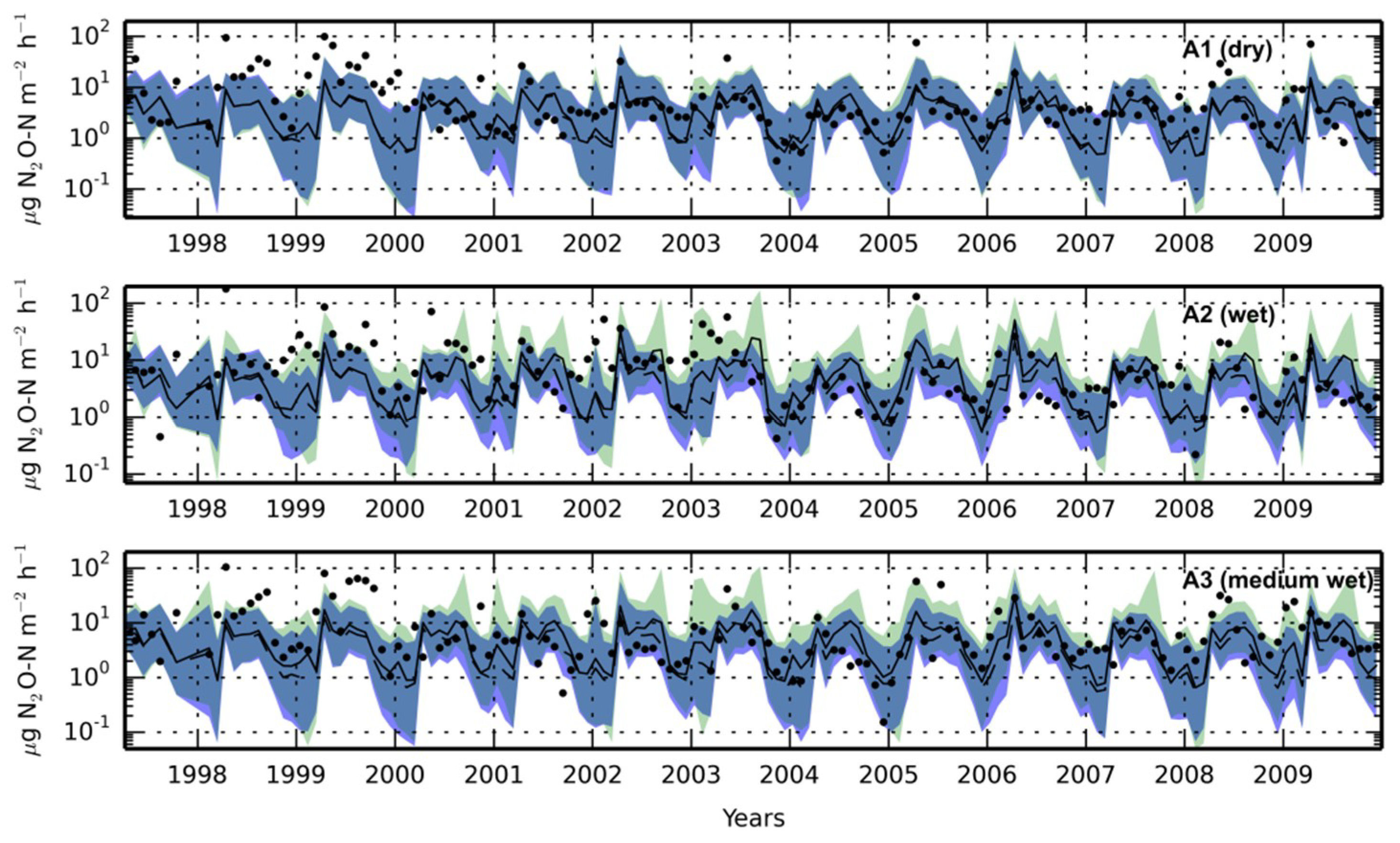
3.4. N2O Emissions
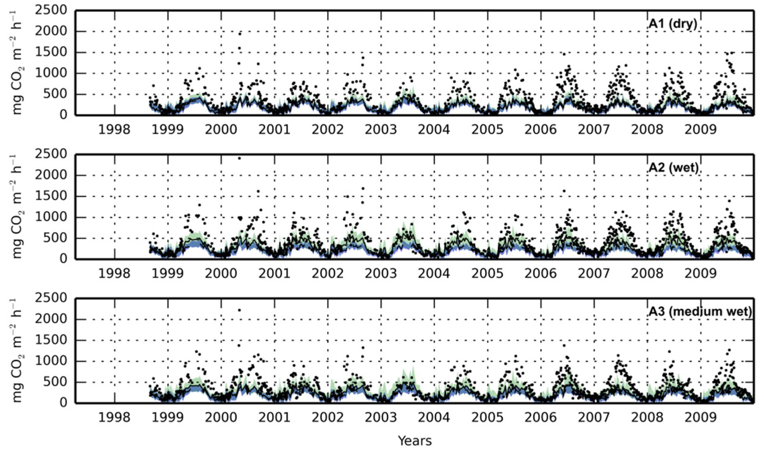
3.5. CO2 Emissions
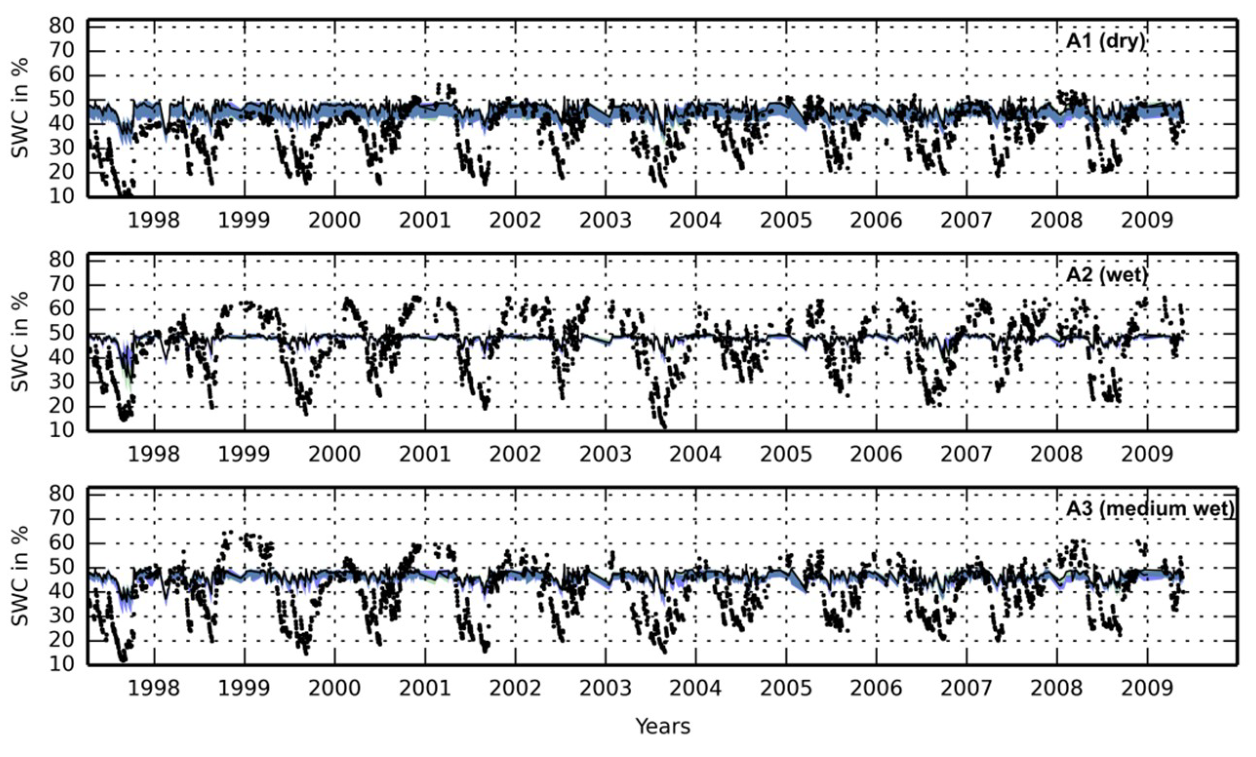
3.6. Soil Water Content
4. Discussion
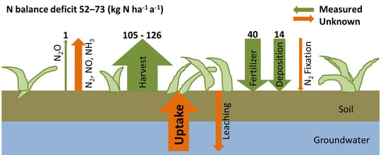
4.1. N Balance and Groundwater NO3−
4.2. Impact of Groundwater-Borne NO3− on Simulated Ecosystem Behaviour
4.3. Groundwater, SWC and N2O Emissions
4.4. CO2 Emissions and SWC
4.5. Intersection Sizes and Model Coherency
5. Conclusions
Author Contributions
Funding
Acknowledgments
Conflicts of Interest
Appendix A

| Name | Value/Unit | Start/End | Temporal Resolution | Usage | Source |
|---|---|---|---|---|---|
| Air Temperature (Mean, Min, Max) | °C | 1995/2009 | daily | Driver data | WD |
| Global Radiation | W m−2 | 1995/2009 | daily | Driver data | WD |
| Precipitation | mm day−1 | 1995/2009 | daily | Driver data | WD |
| Relative Humidity | % | 1995/2009 | daily | Driver data | WD |
| Groundwater level | m | 1995/2009 | daily *1 | Driver data | FSM |
| Cutting schedule | - | 1995/2009 | 2/year | Driver data | FSM |
| Fertilizer application (ammonium nitrate) | 40 kgN ha−1 year−1 | 1995/2009 | yearly | Driver data | [76] |
| N deposition | 14 kgN ha−1 year−1 | 1993/1995 | mean | Driver data | [77] |
| Field capacity | mm m−1 | - | - | Calibrated parameter | [32] |
| Wilting point | mm m−1 | - | - | Calibrated parameter | [32] |
| Fraction of soil org. N | 0.08–0.37% | 2001/2002 | - | Initialization | [31] |
| Fraction of soil org. C | 0.69–3.96% | 2001/2002 | - | Initialization | [31] |
| Plant C/N ratio | 25.7 | 1993/2009 | average | Fixed parameter | FSM |
| Soil pH | 5.4–6.0 | - | - | Fixed parameter | [31] |
| Cutting height | 4 cm | - | constant | Fixed parameter | FSM |
| Bulk density profile | 1.01–1.52 g cm−3 | - | - | Fixed parameter | [32] |
| Texture (clay, silt, sand) | - | - | constant | Fixed parameter | [32] |
| CO2 concentration | 392.5 ppm | 1998/2009 | mean | Fixed parameter | FSM |
| Groundwater NO3− concentration | 3.24 mg L−1 | 2015 | mean | Fixed parameter | FSM |
| CO2 emissions | mg CO2 m−2 h−1 | 1998/2009 | variable | Calibration data | FSM |
| N2O emissions | µgN m−2 h−1 | 1997/2009 | variable monthly mean | Calibration data | FSM |
| Soil water content | % | 1997/2009 | variable *2 | Calibration data | FSM |
| Biomass | kg ha−1 year−1 | 1997/2009 | 2 cuts/year | Calibration data | FSM |
| Parameter Name | Module | Sensitive in Model Setup | Min | Max | Description |
|---|---|---|---|---|---|
| AMAXX | scDNDC | noGW, withGW | 0.6545 | 1.9635 | Microbial death rate |
| D_N2O | scDNDC | withGW | 0.031 | 0.093 | Reduction constant for N2O diffusion |
| D_NO | scDNDC | withGW | 0.0365 | 0.1095 | Reduction constant for NO diffusion |
| DIFF_C | scDNDC | withGW | 0.125 | 0.375 | Diffusion constant for C compounds between aerobic and anaerobic microsites |
| DIFF_N | scDNDC | noGW, withGW | 0.25 | 0.75 | Diffusion constant for N compounds between aerobic and anaerobic microsites |
| DNDC_KMM_N_MIC | scDNDC | noGW | 0.00058875 | 0.00294375 | Michaelis-Menten constant for N dependency of microbial growth |
| EFF_NO2 | scDNDC | noGW | 0.214 | 0.642 | Microbial efficiency for NO2 denitrification |
| EFFAC | scDNDC | noGW, withGW | 0.35 | 0.95 | Fraction of decomposed C that goes to the dissolved organic C pool |
| FCO2_1 | scDNDC | noGW | 0.605 | 1.815 | Factor for CO2 production during humads decomposition process |
| FCO2_3 | scDNDC | noGW | 1.15 | 3.45 | Like FCO2_1 |
| FCO2_HU | scDNDC | noGW | 0.4 | 1.2 | Like FCO2_1 |
| FNO3_U | scDNDC | noGW | 0.375 | 0.9 | Factor steering NO3− availability for microbial assimilation |
| KCHEM | scDNDC | noGW, withGW | 4 | 12 | Reaction rate for chemo-denitrification |
| KCRB_L | scDNDC | withGW | 0.04625 | 0.13875 | Decomposition constant for labile inactive microbes |
| KN2O | scDNDC | noGW, withGW | 0.0025 | 0.0225 | Reaction rate for N2O reductase |
| KNIT | scDNDC | noGW, withGW | 0.5 | 10 | Reaction rate for nitrification |
| M_FACT_DEC1 | scDNDC | noGW, withGW | 0.2975 | 0.8925 | Factor determining dependency of decomposition on water filled pore space |
| M_FACT_P1 | scDNDC | noGW, withGW | 0.225 | 0.675 | Factor determining dependency of nitrification on water filled pore space |
| M_FACT_P6 | scDNDC | noGW | 5 | 15 | Factor determining dependency of microbial activity on water filled pore space |
| MNO | scDNDC | noGW | 0.0395 | 0.1185 | Microbial maintenance coefficient for denitrification of NO |
| PERTVL | scDNDC | withGW | 0.005 | 0.015 | Downward transport of very labile litter |
| PHCRIT_N2O | scDNDC | noGW, withGW | 2.5 | 7.5 | Factor for pH dependency of N2O denitrification |
| PHCRIT_NO2 | scDNDC | noGW, withGW | 3.05 | 9.15 | Factor for pH dependency of NO2 denitrification |
| TF_DEC1 | scDNDC | noGW, withGW | 1.77 | 5.31 | Temperature dependency of decomposition |
| TF_NUP_N2O2 | scDNDC | noGW, withGW | 4.705 | 14.115 | Temperature dependency of N2O production during nitrification |
| sks_upper | wcDNDC | noGW, withGW | 0.0007 | 0.7 | Hydraulic conductivity of uppermost layer |
| wcmax_upper | wcDNDC | noGW, withGW | 450 | 650 | Field capacity of uppermost layer |
| wcmin_upper | wcDNDC | noGW, withGW | 65 | 375 | Wilting point of uppermost layer |
| ROOT | grDNDC | withGW | 0.3 | 0.7 | Root fraction of plant biomass |
| Target Value | Plot | Simulations | Measurements | |||
|---|---|---|---|---|---|---|
| Mean | Median | Quantile 2.5% | Quantile 97.5% | |||
| N2O emissions [µgN m−2 h−1] | A1 | 0.72–25.31 | 0.46–21.19 | 0.03–6.15 | 2.80–68.32 | 0.36–99.04 |
| A2 | 0.80–24.35 | 0.56–21.30 | 0.13–9.12 | 2.21–54.15 | −2.91–178.86 | |
| A3 | 0.78–22.31 | 0.53–17.81 | 0.06–6.06 | 2.97–62.87 | −1.00–104.81 | |
| CO2 emissions [mg m−2 h−1] | A1 | 8.51–408.84 | 2.68–407.55 | 0.42–311.26 | 43.94–546.79 | 27.6–1941.0 |
| A2 | 14.38–384.50 | 10.97–384.83 | 1.35–311.37 | 45.39–477.38 | 32.4–2409.0 | |
| A3 | 12.38–389.74 | 5.51–388.12 | 0.55–295.32 | 49.07–547.58 | 18.4–2221.0 | |
| SWC [%] | A1 | 35.11–51.46 | 35.32–51.39 | 30.97–51.21 | 36.57–52.11 | 9.60–56.28 |
| A2 | 38.47–53.72 | 38.58–53.65 | 35.04–52.83 | 40.03–54.66 | 11.68–64.95 | |
| A3 | 35.42–51.49 | 35.63–51.44 | 30.87–51.21 | 36.85–52.12 | 11.85–64.70 | |
| Biomass [kg ha−1] | A1 | 1421–2281 | 1423–2308 | 1130–1874 | 1671–2714 | 1834–4833 |
| A2 | 1470–2341 | 1463–2348 | 1306–2100 | 1654–2614 | 2068–5630 | |
| A3 | 1461–2301 | 1458–2329 | 1164–1951 | 1733–2871 | 1744–5511 | |
| Target Value | Plot | Simulations | Measurements | |||
|---|---|---|---|---|---|---|
| Mean | Median | Quantile 2.5% | Quantile 97.5% | |||
| N2O emissions [µgN m−2 h−1] | A1 | 0.69–27.84 | 0.45–22.56 | 0.03–5.80 | 2.36–82.87 | 0.36–99.04 |
| A2 | 0.89–57.04 | 0.53–50.52 | 0.07–9.81 | 3.31–169.52 | −2.91–178.86 | |
| A3 | 1.01–37.40 | 0.65–30.44 | 0.05–8.14 | 3.62–107.79 | −1.00–104.81 | |
| CO2 emissions [mg m−2 h−1] | A1 | 9.4–474.7 | 3.4–460.0 | 0.5–319.7 | 51.3–708.7 | 27.6–1941.0 |
| A2 | 18.9–605.3 | 14.3–619.8 | 1.1 –325.7 | 56.7–952.6 | 32.4–2409.0 | |
| A3 | 19.4–523.8 | 7.5–504.3 | 0.6–308.8 | 89.6–914.6 | 18.4–2221.0 | |
| SWC [%] | A1 | 35.36–51.45 | 35.51–51.39 | 30.97–51.20 | 36.92–52.00 | 9.60–56.28 |
| A2 | 30.28–53.63 | 30.58–53.61 | 24.97–52.88 | 34.52–54.64 | 11.68–64.95 | |
| A3 | 37.02–51.49 | 37.13–51.47 | 33.60–51.20 | 38.39–52.24 | 11.85–64.70 | |
| Biomass [kg ha−1] | A1 | 1828–3272 | 1836–3328 | 1280–2162 | 2248–4426 | 1834–4833 |
| A2 | 2499–4931 | 2468–5080 | 1561–2783 | 3154–6342 | 2068–5630 | |
| A3 | 2323–4167 | 2356–4222 | 1418–2573 | 3070–5605 | 1744–5511 | |
| NO3− uptake [kgN ha−1] | A1 | 3.89–54.41 | 4.15–57.78 | 0.33–4.49 | 6.73–93.97 | (24.23–95.13) |
| A2 | 44.95–121.31 | 56.54–130.57 | 3.21–6.78 | 71.53–193.88 | (41.49–103.74) | |
| A3 | 32.26–81.44 | 33.32–84.14 | 3.11–6.40 | 56.98–142.36 | (47.19–115.86) | |
| Target Values | A1 | A2 | A3 |
|---|---|---|---|
| Biomass—CO2 emissions | 8157 | 8252 | 8180 |
| Biomass—N2O emissions | 52963 | 52948 | 53328 |
| Biomass—Soil Moisture Content | 34114 | 34324 | 34117 |
| CO2 emissions—N2O emissions | 23356 | 23146 | 23452 |
| CO2 emissions—Soil Moisture Content | 38774 | 38710 | 38700 |
| N2O emissions—Soil Moisture Content | 38582 | 38608 | 38561 |

References
- Ciais, P.; Sabine, C.; Bala, G.; Bopp, L.; Brovkin, V.; Canadell, J.; Chhabra, A.; DeFries, R.; Galloway, J.; Heimann, M.; et al. Carbon and Other Biogeochemical Cycles. In Climate Change 2013: The Physical Science Basis. Contribution of Working Group I to the Fifth Assessment Report of the Intergovernmental Panel on Climate Change; Cambridge University Press: Cambridge, UK; New York, NY, USA, 2013. [Google Scholar]
- Hartmann, D.L.; Klein Tank, A.M.G.; Rusticucci, M.; Alexander, L.V.; Brönnimann, S.; Charabi, Y.A.-R.; Dentener, F.J.; Dlugokencky, E.J.; Easterling, D.R.; Kaplan, A.; et al. Observations: Atmospheres and Surface. In Climate Change 2013: The Physical Science Basis. Contribution of Working Group I to the Fifth Assessment Report of the Intergovernmental Panel on Climate Change; Cambridge University Press: Cambridge, UK; New York, NY, USA, 2013. [Google Scholar]
- Ravishankara, A.R.; Daniel, J.S.; Portmann, R.W. Nitrous Oxide (N2O): The Dominant Ozone-Depleting Substance Emitted in the 21st Century. Science 2009, 326, 123–125. [Google Scholar] [CrossRef] [PubMed]
- Syakila, A.; Kroeze, C. The global nitrous oxide budget revisited. Greenh. Gas Meas. Manag. 2011, 1, 17–26. [Google Scholar] [CrossRef]
- Butterbach-Bahl, K.; Baggs, E.M.; Dannenmann, M.; Kiese, R.; Zechmeister-Boltenstern, S. Nitrous oxide emissions from soils: How well do we understand the processes and their controls? Philos. Trans. R. Soc. B 2013, 368, 20130122. [Google Scholar] [CrossRef] [PubMed]
- Erisman, J.W.; Galloway, J.N.; Seitzinger, S.; Bleeker, A.; Dise, N.B.; Petrescu, A.M.R.; Leach, A.M.; de Vries, W. Consequences of human modification of the global nitrogen cycle. Philos. Trans. R. Soc. B 2013, 368, 20130116. [Google Scholar] [CrossRef] [PubMed]
- Groffman, P.M.; Butterbach-Bahl, K.; Fulweiler, R.W.; Gold, A.J.; Morse, J.L.; Stander, E.K.; Tague, C.; Tonitto, C.; Vidon, P. Challenges to incorporating spatially and temporally explicit phenomena (hotspots and hot moments) in denitrification models. Biogeochemistry 2009, 93, 49–77. [Google Scholar] [CrossRef]
- Christensen, S. Nitrous oxide emission from a soil under permanent grass: Seasonal and diurnal fluctuations as influenced by manuring and fertilization. Soil Biol. Biochem. 1983, 15, 531–536. [Google Scholar] [CrossRef]
- Gleeson, D.B.; Müller, C.; Banerjee, S.; Ma, W.; Siciliano, S.D.; Murphy, D.V. Response of ammonia oxidizing archaea and bacteria to changing water filled pore space. Soil Biol. Biochem. 2010, 42, 1888–1891. [Google Scholar] [CrossRef]
- Goodroad, L.L.; Keeney, D.R. Nitrous oxide production in aerobic soils under varying pH, temperature and water content. Soil Biol. Biochem. 1984, 16, 39–43. [Google Scholar] [CrossRef]
- Shen, J.-P.; Xu, Z.; He, J.-Z. Frontiers in the microbial processes of ammonia oxidation in soils and sediments. J. Soils Sediments 2014, 14, 1023–1029. [Google Scholar] [CrossRef] [Green Version]
- Smart, D.R.; Bloom, A.J. Wheat leaves emit nitrous oxide during nitrate assimilation. Proc. Natl. Acad. Sci. USA 2001, 98, 7875–7878. [Google Scholar] [CrossRef] [PubMed] [Green Version]
- Smith, K.A.; Thomson, P.E.; Clayton, H.; Mctaggart, I.P.; Conen, F. Effects of temperature, water content and nitrogen fertilisation on emissions of nitrous oxide by soils. Atmos. Environ. 1998, 32, 3301–3309. [Google Scholar] [CrossRef]
- Wrage, N.; Velthof, G.L.; van Beusichem, M.L.; Oenema, O. Role of nitrifier denitrification in the production of nitrous oxide. Soil Biol. Biochem. 2001, 33, 1723–1732. [Google Scholar] [CrossRef]
- Müller, C.; Sherlock, R.R.; Williams, P.H. Mechanistic model for nitrous oxide emission via nitrification and denitrification. Biol. Fertil. Soils 1997, 24, 231–238. [Google Scholar] [CrossRef]
- Ryan, M.; Müller, C.; Di, H.J.; Cameron, K.C. The use of artificial neural networks (ANNs) to simulate N2O emissions from a temperate grassland ecosystem. Ecol. Model. 2004, 175, 189–194. [Google Scholar] [CrossRef]
- Levy, P.E.; Mobbs, D.C.; Jones, S.K.; Milne, R.; Campbell, C.; Sutton, M.A. Simulation of fluxes of greenhouse gases from European grasslands using the DNDC model. Agric. Ecosyst. Environ. 2007, 121, 186–192. [Google Scholar] [CrossRef]
- Xu, R.; Prentice, I.C.; Spahni, R.; Niu, H.S. Modelling terrestrial nitrous oxide emissions and implications for climate feedback. New Phytol. 2012, 196, 472–488. [Google Scholar] [CrossRef] [Green Version]
- Tague, C.L.; Band, L.E. RHESSys: Regional Hydro-Ecologic Simulation System—An Object-Oriented Approach to Spatially Distributed Modeling of Carbon, Water, and Nutrient Cycling. Earth Interact. 2004, 8, 1–42. [Google Scholar] [CrossRef] [Green Version]
- Cui, J.; Li, C.; Sun, G.; Trettin, C. Linkage of MIKE SHE to Wetland-DNDC for carbon budgeting and anaerobic biogeochemistry simulation. Biogeochemistry 2005, 72, 147–167. [Google Scholar] [CrossRef]
- Kraft, P.; Haas, E.; Klatt, S.; Kiese, R.; Butterbach-Bahl, K.; Frede, H.-G.; Breuer, L. Modelling nitrogen transport and turnover at the hillslope scale—A process oriented approach. In 6th International Congress on Environmental Modelling and Software 2012; International Environmental Modelling and Software Society (iEMSs): Leipzig, Germany, 2012; ISBN 978-88-9035-742-8. [Google Scholar]
- Wlotzka, M.; Haas, E.; Kraft, P.; Heuveline, V.; Klatt, S.; Kraus, D.; Butterbach-Bahl, K.; Breuer, L. Dynamic Simulation of Land Management Effects on Soil N2O Emissions using a coupled Hydrology-Ecosystem Model. Prepr. Ser. Eng. Math. Comput. Lab. 2013. [Google Scholar] [CrossRef]
- Klatt, S.; Kraus, D.; Kraft, P.; Breuer, L.; Wlotzka, M.; Heuveline, V.; Haas, E.; Kiese, R.; Butterbach-Bahl, K. Exploring impacts of vegetated buffer strips on nitrogen cycling using a spatially explicit hydro-biogeochemical modeling approach. Environ. Model. Softw. 2017, 90, 55–67. [Google Scholar] [CrossRef]
- Brown, K.S.; Sethna, J.P. Statistical mechanical approaches to models with many poorly known parameters. Phys. Rev. E 2003, 68, 021904. [Google Scholar] [CrossRef] [PubMed]
- Rahn, K.-H.; Werner, C.; Kiese, R.; Haas, E.; Butterbach-Bahl, K. Parameter-induced uncertainty quantification of soil N2O, NO and CO2 emission from Höglwald spruce forest (Germany) using the LandscapeDNDC model. Biogeosciences 2012, 9, 3983–3998. [Google Scholar] [CrossRef]
- Confalonieri, R. Monte Carlo based sensitivity analysis of two crop simulators and considerations on model balance. Eur. J. Agron. 2010, 33, 89–93. [Google Scholar] [CrossRef]
- Pappenberger, F.; Beven, K.J. Ignorance is bliss: Or seven reasons not to use uncertainty analysis. Water Resour. Res. 2006, 42, W05302. [Google Scholar] [CrossRef]
- Beven, K.; Freer, J. Equifinality, data assimilation, and uncertainty estimation in mechanistic modelling of complex environmental systems using the GLUE methodology. J. Hydrol. 2001, 249, 11–29. [Google Scholar] [CrossRef]
- Haas, E.; Klatt, S.; Fröhlich, A.; Kraft, P.; Werner, C.; Kiese, R.; Grote, R.; Breuer, L.; Butterbach-Bahl, K. LandscapeDNDC: A process model for simulation of biosphere–atmosphere–hydrosphere exchange processes at site and regional scale. Landsc. Ecol. 2013, 28, 615–636. [Google Scholar] [CrossRef]
- Grünhage, L.; Schmitt, J.; Hertstein, U.; Janze, S.; Peter, M.; Jäger, H.-J., III. Beschreibung der Versuchsfläche. In Auswirkungen dynamischer Veränderungen der Luftzusammensetzung und des Klimas auf terrestrische Ökosysteme in Hessen-II-Umweltbeobachtungs- und Klimafolgenforschungsstation Linden, Jahresbericht 1995; Umweltplanung, Arbeits- und Umweltschutz: Wiesbaden, Germany, 1996; ISBN 3-89026-236-8. [Google Scholar]
- Jäger, H.-J.; Schmidt, S.W.; Kammann, C.; Grünhage, L.; Müller, C.; Hanewald, K. The University of Giessen Free-Air Carbon dioxide Enrichment study: Description of the experimental site and of a new enrichment system. J. Appl. Bot. 2003, 77, 117–127. [Google Scholar]
- Kammann, C.; Grünhage, L.; Jäger, H.-J., II. N2O- und CH4-Flüsse in der bodennahen Atmosphäre eines extensiv genutzten Grünlandökosystems. In Auswirkungen dynamischer Veränderungen der Luftzusammensetzung und des Klimas auf terrestrische Ökosysteme in Hessen-III-Umweltbeobachtungs- und Klimafolgenforschungsstation Linden, Berichtszeitraum 1996–1999; Umweltplanung, Arbeits- und Umweltschutz: Wiesbaden, Germany, 2000; ISBN 3-89026-311-9. [Google Scholar]
- Näsholm, T.; Huss-Danell, K.; Högberg, P. Uptake of Organic Nitrogen in the Field by Four Agriculturally Important Plant Species. Ecology 2000, 81, 1155–1161. [Google Scholar] [CrossRef]
- Grote, R.; Kiese, R.; Grünwald, T.; Ourcival, J.-M.; Granier, A. Modelling forest carbon balances considering tree mortality and removal. Agric. For. Meteorol. 2011, 151, 179–190. [Google Scholar] [CrossRef]
- Stange, F.; Butterbach-Bahl, K.; Papen, H.; Zechmeister-Boltenstern, S.; Li, C.; Aber, J. A process-oriented model of N2O and NO emissions from forest soils: 2. Sensitivity analysis and validation. J. Geophys. Res. Atmos. 2000, 105, 4385–4398. [Google Scholar] [CrossRef]
- Werner, C.; Butterbach-Bahl, K.; Haas, E.; Hickler, T.; Kiese, R. A global inventory of N2O emissions from tropical rainforest soils using a detailed biogeochemical model. Glob. Biogeochem. Cycles 2007, 21, GB3010. [Google Scholar] [CrossRef]
- Saggar, S.; Giltrap, D.L.; Li, C.; Tate, K.R. Modelling nitrous oxide emissions from grazed grasslands in New Zealand. Agric. Ecosyst. Environ. 2007, 119, 205–216. [Google Scholar] [CrossRef]
- Abdalla, M.; Kumar, S.; Jones, M.; Burke, J.; Williams, M. Testing DNDC model for simulating soil respiration and assessing the effects of climate change on the CO2 gas flux from Irish agriculture. Glob. Planet. Chang. 2011, 78, 106–115. [Google Scholar] [CrossRef]
- Molina-Herrera, S.; Haas, E.; Klatt, S.; Kraus, D.; Augustin, J.; Magliulo, V.; Tallec, T.; Ceschia, E.; Ammann, C.; Loubet, B.; et al. A modeling study on mitigation of N2O emissions and NO3 leaching at different agricultural sites across Europe using LandscapeDNDC. Sci. Total Environ. 2016, 553, 128–140. [Google Scholar] [CrossRef] [PubMed]
- Li, C.; Frolking, S.; Frolking, T.A. A model of nitrous oxide evolution from soil driven by rainfall events: 1. Model structure and sensitivity. J. Geophys. Res. Atmos. 1992, 97, 9759–9776. [Google Scholar] [CrossRef]
- Kiese, R.; Heinzeller, C.; Werner, C.; Wochele, S.; Grote, R.; Butterbach-Bahl, K. Quantification of nitrate leaching from German forest ecosystems by use of a process oriented biogeochemical model. Environ. Pollut. 2011, 159, 3204–3214. [Google Scholar] [CrossRef] [PubMed]
- Grote, R.; Lavoir, A.-V.; Rambal, S.; Staudt, M.; Zimmer, I.; Schnitzler, J.-P. Modelling the drought impact on monoterpene fluxes from an evergreen Mediterranean forest canopy. Oecologia 2009, 160, 213–223. [Google Scholar] [CrossRef] [PubMed]
- Houska, T.; Kraft, P.; Chamorro-Chavez, A.; Breuer, L. SPOTting Model Parameters Using a Ready-Made Python Package. PLoS ONE 2015, 10, e0145180. [Google Scholar] [CrossRef] [PubMed]
- Cukier, R.I.; Fortuin, C.M.; Shuler, K.E.; Petschek, A.G.; Schaibly, J.H. Study of the sensitivity of coupled reaction systems to uncertainties in rate coefficients. I Theory. J. Chem. Phys. 1973, 59, 3873–3878. [Google Scholar] [CrossRef]
- Saltelli, A.; Tarantola, S.; Chan, K.P.-S. A Quantitative Model-Independent Method for Global Sensitivity Analysis of Model Output. Technometrics 1999, 41, 39–56. [Google Scholar] [CrossRef]
- McKay, M.D.; Beckman, R.J.; Conover, W.J. A Comparison of Three Methods for Selecting Values of Input Variables in the Analysis of Output from a Computer Code. Technometrics 1979, 21, 239–245. [Google Scholar] [CrossRef]
- He, J.; Jones, J.W.; Graham, W.D.; Dukes, M.D. Influence of likelihood function choice for estimating crop model parameters using the generalized likelihood uncertainty estimation method. Agric. Syst. 2010, 103, 256–264. [Google Scholar] [CrossRef]
- Pathak, T.B.; Jones, J.W.; Fraisse, C.W.; Wright, D.; Hoogenboom, G. Uncertainty Analysis and Parameter Estimation for the CSM-CROPGRO-Cotton Model. Agron. J. 2012, 104, 1363. [Google Scholar] [CrossRef] [Green Version]
- Giese, M.; Brueck, H.; Gao, Y.Z.; Lin, S.; Steffens, M.; Koegel-Knabner, I.; Glindemann, T.; Susenbeth, A.; Taube, F.; Butterbach-Bahl, K.; et al. N balance and cycling of Inner Mongolia typical steppe: A comprehensive case study of grazing effects. Ecol. Monogr. 2013, 83, 195–219. [Google Scholar] [CrossRef]
- Kreutzer, K.; Butterbach-Bahl, K.; Rennenberg, H.; Papen, H. The complete nitrogen cycle of an N-saturated spruce forest ecosystem. Plant Biol. 2009, 11, 643–649. [Google Scholar] [CrossRef] [PubMed] [Green Version]
- Zhou, M.; Zhu, B.; Brüggemann, N.; Dannenmann, M.; Wang, Y.; Butterbach-Bahl, K. Sustaining crop productivity while reducing environmental nitrogen losses in the subtropical wheat-maize cropping systems: A comprehensive case study of nitrogen cycling and balance. Agric. Ecosyst. Environ. 2016, 231, 1–14. [Google Scholar] [CrossRef]
- Paustian, K.; Andren, O.; Clarholm, M.; Hansson, A.-C.; Johansson, G.; Lagerlof, J.; Lindberg, T.; Pettersson, R.; Sohlenius, B. Carbon and Nitrogen Budgets of Four Agro-Ecosystems With Annual and Perennial Crops, With and Without N Fertilization. J. Appl. Ecol. 1990, 27, 60. [Google Scholar] [CrossRef]
- Watson, C.J.; Jordan, C.; Kilpatrick, D.; McCarney, B.; Stewart, R. Impact of grazed grassland management on total N accumulation in soil receiving different levels of N inputs. Soil Use Manag. 2007, 23, 121–128. [Google Scholar] [CrossRef]
- Müller, C.; Stevens, R.J.; Laughlin, R.J.; Jäger, H.-J. Microbial processes and the site of N2O production in a temperate grassland soil. Soil Biol. Biochem. 2004, 36, 453–461. [Google Scholar] [CrossRef]
- Regan, K.; Kammann, C.; Hartung, K.; Lenhart, K.; Müller, C.; Philippot, L.; Kandeler, E.; Marhan, S. Can differences in microbial abundances help explain enhanced N2O emissions in a permanent grassland under elevated atmospheric CO2? Glob. Chang. Biol. 2011, 17, 3176–3186. [Google Scholar] [CrossRef]
- Luo, Q.; Gong, J.; Zhai, Z.; Pan, Y.; Liu, M.; Xu, S.; Wang, Y.; Yang, L.; Baoyin, T. The responses of soil respiration to nitrogen addition in a temperate grassland in northern China. Sci. Total Environ. 2016, 569, 1466–1477. [Google Scholar] [CrossRef] [PubMed]
- Breuer, L.; Papen, H.; Butterbach-Bahl, K. N2O emission from tropical forest soils of Australia. J. Geophys. Res. Atmos. 2000, 105, 26353–26367. [Google Scholar] [CrossRef]
- Kröbel, R.; Sun, Q.; Ingwersen, J.; Chen, X.; Zhang, F.; Müller, T.; Römheld, V. Modelling water dynamics with DNDC and DAISY in a soil of the North China Plain: A comparative study. Environ. Model. Softw. 2010, 25, 583–601. [Google Scholar] [CrossRef]
- Duretz, S.; Drouet, J.L.; Durand, P.; Hutchings, N.J.; Theobald, M.R.; Salmon-Monviola, J.; Dragosits, U.; Maury, O.; Sutton, M.A.; Cellier, P. NitroScape: A model to integrate nitrogen transfers and transformations in rural landscapes. Environ. Pollut. 2011, 159, 3162–3170. [Google Scholar] [CrossRef] [PubMed]
- Xiang, S.-R.; Doyle, A.; Holden, P.A.; Schimel, J.P. Drying and rewetting effects on C and N mineralization and microbial activity in surface and subsurface California grassland soils. Soil Biol. Biochem. 2008, 40, 2281–2289. [Google Scholar] [CrossRef]
- Sándor, R.; Barcza, Z.; Hidy, D.; Lellei-Kovács, E.; Ma, S.; Bellocchi, G. Modelling of grassland fluxes in Europe: Evaluation of two biogeochemical models. Agric. Ecosyst. Environ. 2016, 215, 1–19. [Google Scholar] [CrossRef]
- Zhang, X.; Niu, G.-Y.; Elshall, A.S.; Ye, M.; Barron-Gafford, G.A.; Pavao-Zuckerman, M. Assessing five evolving microbial enzyme models against field measurements from a semiarid savannah—What are the mechanisms of soil respiration pulses? Geophys. Res. Lett. 2014, 41, 6428–6434. [Google Scholar] [CrossRef]
- Amthor, J.S. The McCree–de Wit–Penning de Vries–Thornley Respiration Paradigms: 30 Years Later. Ann. Bot. 2000, 86, 1–20. [Google Scholar] [CrossRef] [Green Version]
- Dong, Y.; Zhang, S.; Qi, Y.; Chen, Z.; Geng, Y. Fluxes of CO2, N2O and CH4 from a typical temperate grassland in Inner Mongolia and its daily variation. Chin. Sci. Bull. 2000, 45, 1590–1594. [Google Scholar] [CrossRef]
- Müller, C. Plants affect the in situ N2O emissions of a temperate grassland ecosystem. Pflanzen beeinflussen die in situ N2O-Freisetzungen eines Grünlandökosystems in temperierten Breiten. J. Plant Nutr. Soil Sci. 2003, 166, 771–773. [Google Scholar] [CrossRef]
- Šimek, M.; Hynšt, J.; Šimek, P. Emissions of CH4, CO2, and N2O from soil at a cattle overwintering area as affected by available C and N. Appl. Soil Ecol. 2014, 75, 52–62. [Google Scholar] [CrossRef]
- Klepper, O. Multivariate aspects of model uncertainty analysis: Tools for sensitivity analysis and calibration. Ecol. Model. 1997, 101, 1–13. [Google Scholar] [CrossRef]
- Wutzler, T.; Carvalhais, N. Balancing multiple constraints in model-data integration: Weights and the parameter block approach. J. Geophys. Res. Biogeosci. 2014, 119, 2112–2129. [Google Scholar] [CrossRef] [Green Version]
- Yapo, P.O.; Gupta, H.V.; Sorooshian, S. Multi-objective global optimization for hydrologic models. J. Hydrol. 1998, 204, 83–97. [Google Scholar] [CrossRef]
- Houska, T.; Multsch, S.; Kraft, P.; Frede, H.-G.; Breuer, L. Monte Carlo-based calibration and uncertainty analysis of a coupled plant growth and hydrological model. Biogeosciences 2014, 11, 2069–2082. [Google Scholar] [CrossRef] [Green Version]
- Sitch, S.; Smith, B.; Prentice, I.C.; Arneth, A.; Bondeau, A.; Cramer, W.; Kaplan, J.O.; Levis, S.; Lucht, W.; Sykes, M.T.; et al. Evaluation of ecosystem dynamics, plant geography and terrestrial carbon cycling in the LPJ dynamic global vegetation model. Glob. Chang. Biol. 2003, 9, 161–185. [Google Scholar] [CrossRef]
- Kraft, P.; Vaché, K.B.; Frede, H.-G.; Breuer, L. CMF: A Hydrological Programming Language Extension For Integrated Catchment Models. Environ. Model. Softw. 2011, 26, 828–830. [Google Scholar] [CrossRef]
- Kraus, D.; Weller, S.; Klatt, S.; Haas, E.; Wassmann, R.; Kiese, R.; Butterbach-Bahl, K. A new LandscapeDNDC biogeochemical module to predict CH4 and N2O emissions from lowland rice and upland cropping systems. Plant Soil 2014, 386, 125–149. [Google Scholar] [CrossRef]
- Farquhar, G.D.; von Caemmerer, S.; Berry, J.A. A biochemical model of photosynthetic CO2 assimilation in leaves of C3 species. Planta 1980, 149, 78–90. [Google Scholar] [CrossRef] [PubMed]
- Dämmgen, U.; Grünhage, L.; Schaaf, S. The precision and spatial variability of some meteorological parameters needed to determine vertical fluxes of air constituents. Landbauforsch. Volkenrode 2005, 55, 29–37. [Google Scholar]
- Kammann, C.; Müller, C.; Grünhage, L.; Jäger, H.-J. Elevated CO2 stimulates N2O emissions in permanent grassland. Soil Biol. Biochem. 2008, 40, 2194–2205. [Google Scholar] [CrossRef]
- Scholz-Seidel, C. Dämmgen, U.V.2 Messungen der Bulk-Depositionen sedimentierender anorganischer Spezies (September 1993 bis Dezember 1995). In Auswirkungen dynamischer Veränderungen der Luftzusammensetzung und des Klimas auf terrestrische Ökosysteme in Hessen-II-Umweltbeobachtungs- und Klimafolgenforschungsstation Linden, Jahresbericht 1995; Umweltplanung, Arbeits- und Umweltschutz: Wiesbaden, Germany, 1996; ISBN 3-89026-236-8. [Google Scholar]


| Name | Average N Fluxes in kgN ha−1 | ||
|---|---|---|---|
| A1 | A2 | A3 | |
| Atmospheric N deposition | 14 | 14 | 14 |
| N fertilizer application | 40 | 40 | 40 |
| N2O emission | −1 | −1 | −1 |
| N removal by harvest | −106 | −123 | −129 |
| N balance | −53 | −70 | −76 |
| Model Setups | A1 | A2 | A3 |
|---|---|---|---|
| noGW | 471 | 73 | 427 |
| withGW | 469 | 58 | 395 |
| reference value | 2344 | ||
| Target Value | Plot | Minimum RMSE | Mean RMSE | Maximum RMSE | Measurements (Mean) | |||
|---|---|---|---|---|---|---|---|---|
| noGW | withGW | noGW | withGW | noGW | withGW | |||
| Biomass [kg ha−1] | A1 | 1308 | 660 | 1572 | 1081 | 1952 | 1780 | 3040 |
| A2 | 1822 | 810 | 2002 | 1233 | 2226 | 1830 | 3585 | |
| A3 | 1815 | 796 | 2088 | 1294 | 2434 | 2069 | 3348 | |
| Target Value | Plot | Minimum RMSE | Mean RMSE | Maximum RMSE | Measurements (Mean) | |||
|---|---|---|---|---|---|---|---|---|
| noGW | withGW | noGW | withGW | noGW | withGW | |||
| N2O emissions [µgN m−2 h−1] | A1 | 13.47 | 13.55 | 15.76 | 15.78 | 18.21 | 18.20 | 9.33 |
| A2 | 19.86 | 19.43 | 21.33 | 22.90 | 22.60 | 38.35 | 11.16 | |
| A3 | 14.13 | 14.31 | 16.03 | 17.10 | 17.58 | 50.38 | 10.20 | |
| Target Value | Plot | Minimum RMSE | Mean RMSE | Maximum RMSE | Measurements (Mean) | |||
|---|---|---|---|---|---|---|---|---|
| noGW | withGW | noGW | withGW | noGW | withGW | |||
| CO2 emissions [mg m−2 h−1] | A1 | 264.6 | 214.5 | 318.0 | 296.5 | 353.5 | 356.5 | 382.2 |
| A2 | 291.7 | 201.8 | 327.5 | 265.4 | 362.1 | 380.5 | 398.2 | |
| A3 | 241.6 | 176.4 | 288.3 | 252.3 | 325.2 | 337.0 | 363.9 | |
| Target Value | Plot | Minimum RMSE | Mean RMSE | Maximum RMSE | Measurements (Means) | |||
|---|---|---|---|---|---|---|---|---|
| noGW | withGW | noGW | withGW | noGW | withGW | |||
| SWC [%] | A1 | 9.66 | 10.05 | 13.42 | 13.46 | 14.67 | 14.80 | 34.86 |
| A2 | 11.28 | 11.54 | 12.07 | 12.01 | 12.73 | 12.59 | 43.62 | |
| A3 | 10.75 | 11.39 | 12.82 | 13.18 | 13.75 | 14.00 | 37.55 | |
© 2018 by the authors. Licensee MDPI, Basel, Switzerland. This article is an open access article distributed under the terms and conditions of the Creative Commons Attribution (CC BY) license (http://creativecommons.org/licenses/by/4.0/).
Share and Cite
Liebermann, R.; Breuer, L.; Houska, T.; Klatt, S.; Kraus, D.; Haas, E.; Müller, C.; Kraft, P. Closing the N-Budget: How Simulated Groundwater-Borne Nitrate Supply Affects Plant Growth and Greenhouse Gas Emissions on Temperate Grassland. Atmosphere 2018, 9, 407. https://doi.org/10.3390/atmos9100407
Liebermann R, Breuer L, Houska T, Klatt S, Kraus D, Haas E, Müller C, Kraft P. Closing the N-Budget: How Simulated Groundwater-Borne Nitrate Supply Affects Plant Growth and Greenhouse Gas Emissions on Temperate Grassland. Atmosphere. 2018; 9(10):407. https://doi.org/10.3390/atmos9100407
Chicago/Turabian StyleLiebermann, Ralf, Lutz Breuer, Tobias Houska, Steffen Klatt, David Kraus, Edwin Haas, Christoph Müller, and Philipp Kraft. 2018. "Closing the N-Budget: How Simulated Groundwater-Borne Nitrate Supply Affects Plant Growth and Greenhouse Gas Emissions on Temperate Grassland" Atmosphere 9, no. 10: 407. https://doi.org/10.3390/atmos9100407