Incorporation of Numerical Plume Rise Algorithms in the Lagrangian Particle Model LAPMOD and Validation against the Indianapolis and Kincaid Datasets

Abstract

This paper describes the methodology used to incorporate two numerical plume rise algorithms, one by Janicke and Janicke and another by Webster and Thomson, into the Lagrangian particle model LAPMOD. LAPMOD is fully interfaced with the diagnostic meteorological model CALMET, which is part of the widely used CALPUFF modeling system. LAPMOD can also use the meteorological input files produced with the AERMET meteorological processor of the US-EPA recommended model AERMOD. This paper outlines the theory behind the two plume rise algorithms and the details of their implementation in LAPMOD. The paper also provides the results of the evaluation of LAPMOD and its included plume rise algorithms against the well-known Indianapolis and Kincaid SF₆ and SO₂ field studies and tracer experiments. The performance of LAPMOD is successfully evaluated with the Model Evaluation Kit and compared with that of other air quality models.

1. Introduction

In most countries, Gaussian models are the reference tool recommended for atmospheric regulatory modeling applications. The most widely used of such Gaussian models is AERMOD, developed and distributed by the US-EPA [1]. The success of Gaussian models is due to several important factors, such as the simplicity of the algorithm, the direct physical interpretation of the parameters involved, and the limited number of input parameters required. Moreover, practical applications for regulatory purposes typically require the calculation of statistical parameters based on multi-year hourly values of concentration of pollutants emitted by several sources. Gaussian models are particularly fit for such simulations because of their fast execution, even on desktop computers.

However, Gaussian models show various limitations. For example, the stationarity of the solution over one hour implies constant meteorology and does not allow the simulation of accumulation and recirculation effects. In addition, the horizontal homogeneity of the meteorological conditions for any fixed height above terrain does not allow the treatment of variable land-use and orographic effects and limits the extent of the modeling domain where meteorological conditions are representative. The Gaussian solution to the dispersion equation is valid only for non-zero wind speed. For this reason, calm or very low wind conditions cannot be accounted for. Turbulence is assumed to be Gaussian via the dispersion coefficients, and this poses a limit in modeling convective conditions that are known to be characterized by updrafts and downdrafts that make the distribution of vertical wind velocity fluctuations non-Gaussian and non-homogeneous. Another limitation is the assumption of an infinite extent of the plume, up to distances that can be inconsistent with the wind velocity (i.e., impacts several kilometers downwind in low-wind conditions).

Most of these limitations are overcome by Lagrangian models. A popular model is the Lagrangian puff model CALPUFF [2]. This model implements a hybrid approach, because the mass of emitted pollutant is divided into puffs that are transported by the average local wind and expand in size with a Gaussian distribution.

In addition to Lagrangian puff models, Lagrangian particle dispersion models (LPDMs) have become more and more appealing as a modeling tool to simulate atmospheric dispersion of pollutants. Their main feature is the ability to reproduce the stochastic nature of turbulence under all conditions (e.g., [3]).

Lagrangian particle models simulate the released pollutants by following several independent computational particles—each one representing a fraction of the released mass—in a sequence of finite time intervals. The motion of each particle is driven by a time-varying velocity field, which can be divided into an average component, the average wind, plus a fluctuation velocity describing the effects of atmospheric turbulence and those wind variations not included in the mean component. The fluctuation velocity can be described by a nonlinear form of the Langevin stochastic differential equation.

While particles in Lagrangian particle models are generally considered computational markers of the atmospheric fluid that allow the simulation of the concentration field of the pollutant, the description of released matter in terms of particles allows easy incorporation of some physical processes, such as radioactive decay and deposition. Since computational particles represent the pollutants as gas or particulate, deposition and gravitational settling can also be taken into account.

Lagrangian particle models often require: (1) a large number of particles to obtain satisfactory resolution and statistically-sound results; and (2) a short time interval to numerically integrate the equation of motion of the particles. The computational resources commonly available nowadays make these models suitable for implementations oriented both to real time applications (e.g., 24-h forecasting), and to simulate long periods (e.g., months or years of emission from a source).

One of the available, peer-reviewed Lagrangian particle models is LAPMOD [4]. LAPMOD is a freely-available open-source model that is interfaced to the CALMET meteorological preprocessor [5] of the CALPUFF modeling system [2]. LAPMOD is also capable of using the AERMOD meteorological input files via its LAPMET preprocessor. The theoretical formulation of the LAPMOD model and its validation in rural environment against the Kincaid SF₆ and SO₂ datasets [6,7] have been described in a previous paper [4].

A correct description of the plume rise is fundamental in atmospheric dispersion models. Once a plume is emitted by a stack into the atmosphere, three different phases may be individuated while it rises in the atmosphere (e.g., [8]). The initial phase is composed of three sub-phases. Initially, a vertical jet may form until effluents are deflected after release. The successive steps are the bent-over sub-phase, where the plume starts to bend due to the entrainment with the air, and the thermal sub-phase, where the plume grows due to its internal turbulence. During the transition phase, the plume has lost much of its internal turbulence, but it continues to grow, vertically and horizontally, due to the increasing role of atmospheric turbulence. Finally, in the diffusion phase, the plume has lost all its energy and the pollutant is advected and dispersed only due to the average wind speed and atmospheric turbulence. The first two phases are typically summarized with the term “plume rise”. They happen due to the thermal buoyancy of the effluent (i.e., its temperature is greater than the temperature of the surrounding air), and to the momentum of the effluent (i.e., its exit speed).

Different algorithms have been proposed in the past, and may be grouped into three classes: semi-empirical, analytical, and numerical. Independent of the type of algorithm, the most important variables to describe the plume rise are the stack diameter, the exit temperature, the exit speed, the ambient temperature, and the temperature vertical gradient in the atmosphere. For the particular cases of dense plumes, densities must be considered too. There are two parameters that may be defined to characterize the plume when it is released: the buoyancy flux and the momentum flux. The buoyancy flux is directly proportional to the difference between the effluent temperature and the atmospheric temperature, the exit speed, and the exit area of the stack. The momentum flux is directly proportional to the square of the exit speed and to the exit area of the stack.

Analytical algorithms [9,10] allow the determination of the final plume rise, or the plume rise at a given downwind distance from the stack, with different expressions based on the above-mentioned variables and depending on the atmospheric stability. The semi-empirical algorithms assume constant values of the variables (e.g., wind speed, temperature) and express the plume rise height at a given downwind distance from the source as proportional to the product by the heat emission rate, the wind speed, and the distance itself, each one elevated at a specific power (e.g., [11]). These algorithms, similar to the analytical ones, assume constant values of the input variables.

The plume rise numerical algorithms are models within the models that solve different equations describing the emissions, e.g., the conservation of mass, energy, and momentum. They do not require simplification assumptions but need more computational resources than the analytical and semi-empirical solutions. These algorithms do not require constant meteorological variables; both wind and temperature may vary.

This paper describes the incorporation of two numerical plume rise algorithms [12,13] in the Lagrangian particle model LAPMOD [4]. The plume rise algorithms are validated against the Indianapolis field experiment carried out in an urban environment [14]. Once a set of input variables giving satisfactory results for Indianapolis is determined, we use the same model configuration to evaluate LAPMOD against the Kincaid dataset [15], both for SF₆ and SO₂. The purpose of this second validation is to determine a default model configuration that may be used for future studies both in rural and in urban environments.

2. Material and Methods

2.1. The LAPMOD Model

The LAPMOD modeling system is an open source Fortran code available at https://www.enviroware.com/lapmod. This paragraph describes only the parts of the model related to plume rise, while for all the other details the reader should refer to [4].

2.1.1. Plume Rise Algorithms

Plume rise can be simulated in LAPMOD either with the algorithm proposed by Janicke and Janicke [12] (JJ) or with the one proposed by Webster and Thomson [13] (WT). Both algorithms are three-dimensional; therefore, they can be applied in situations with highly complex wind fields, and do not require unrealistic simplifications of wind velocity depending only on vertical elevation and constant direction or even constant wind speed for the whole plume height.

The equations of the two algorithms are written as a function of the distance along the plume axis. The relations between the Cartesian coordinates and the distance along the plume axis, s, are:

dx_i/ds = u_i/u,

(1)

where u is the plume velocity measured along its axis, and u_i represents each one of the Cartesian components of the plume velocity.

The coupled conservation equations solved by the algorithms in LAPMOD with a fourth-order Runge–Kutta method include the dry-air mass conservation, the conservation of momentum and the equation of balance of enthalpy. The main difference between the two algorithms is that JJ also includes the mass conservation of water (vapor phase plus liquid phase), allowing to consider both wet and dry (saturated and non-saturated) plumes. The JJ algorithm includes the ambient humidity, even for the cases when the release of a dry plume is considered.

Another difference between the two plume rise formulations is the entrainment formulation (i.e., the rate at which the plume is diluted by ambient air). For the JJ algorithm, LAPMOD allows a choice among three different formulations: Janicke and Janicke [12], Rezacova and Sokol [16], and Orville [17]. On the contrary, when the WT algorithm is selected, a single entrainment formulation is available, which depends on two velocities, the first one due to the relative motion between the plume and the environment, and the second one due to the ambient turbulence. The mathematical details of the JJ algorithm, as well as the entrainment equations, are described in [18], while those of the WT algorithm are described in [13]. A brief overview of the two plume rise schemes is provided hereafter.

In the following equations, the subscript “a” indicates a property of the atmosphere, while the plume related variables are without any subscript.

The Janicke and Janicke [12] plume rise scheme solves the equations for dry-air mass, momentum, water content and enthalpy.

The dry-air mass conservation equation is:

dM/ds = ε,

(2)

where ε (kg m⁻¹ s⁻¹) is the entrainment rate, and the mass flux M (kg s⁻¹) is given by:

M = A ρ u,

(3)

where A is the plume section (m²) and ρ (kg m⁻³) is the plume density.

The conservation of momentum is described by the equation:

d(M u_i)/ds = ε u_ai + δ_1,3 A g (ρ_a − ρ),

(4)

where “i” indicates one of the three Cartesian directions and δ is the Kronecker delta. The total water content in the plume is given by ζ = η + q, where η is the liquid water content and q is the specific humidity and the equation for mass conservation of water is:

d(M ζ)/ds = ε ζ_a.

(5)

The equation for the balance of enthalpy is:

$$\frac{\mathrm{d}}{\mathrm{ds}}\left[\mathrm{M}\left(\mathrm{T}-\frac{{\mathrm{h}}_{\mathsf{\upsilon }}}{{\mathrm{C}}_{\mathrm{p}}}\mathsf{\eta }\right)\right]=-\mathrm{M}\frac{\mathrm{g}{\mathrm{u}}_{\mathrm{z}}{\mathsf{\rho }}_{\mathrm{a}}}{{\mathrm{C}}_{\mathrm{p}}\mathrm{u}\mathsf{\rho }}+\mathsf{\epsilon }\left({\mathrm{T}}_{\mathrm{a}}-\frac{{\mathrm{h}}_{\mathsf{\upsilon }}}{{\mathrm{C}}_{\mathrm{p}}}{\mathsf{\eta }}_{\mathrm{a}}\right),$$

(6)

where h_υ is the latent heat of evaporation (kJ kg⁻¹) and c_p is the specific heat capacity at constant pressure (kJ kg⁻¹ K⁻¹). The equations presented are solved numerically after the specification of proper initial conditions.

The Webster and Thomson [13] plume rise scheme solves the following set of equations:

dF_m/ds = ε

(7)

dF_Mi/ds = −F_m du_ai/ds − D_i + δ_i,3 π b² g (ρ_a − ρ)

(8)

dF_h/ds = −F_m c_p dθ_a/ds

(9)

where D_i are the drag force components (kg s⁻²), u_ai are the components of the mean wind velocity of the ambient flow (m s⁻¹), θ is the potential temperature (K), and b = b(t) is the plume radius (m). The mass flux F_m, the components of the momentum flux F_Mi, and the heat flux F_h are given by:

F_m = π b² ρ u_s

(10)

F_Mi = (u_i − u_ai) F_m

(11)

F_h = c_p (θ − θ_a) F_m

(12)

where u_s is the modulus of the plume velocity (m s⁻¹) whose components are denoted with u_i (m s⁻¹).

2.1.2. Plume Rise Induced Turbulence

The turbulence inside the plume is high close to the release—where temperature and speed are elevated—and decreases moving away from the point of release due to the entrainment of air at ambient conditions.

As already indicated, a computational particle moves in the “free” atmosphere due to the effect of a mean wind and turbulent fluctuations. Similarly, in LAPMOD, a particle trapped inside a rising plume is moved using the mean velocity components of the plume, computed using the JJ or WT algorithms, plus turbulent fluctuations. These fluctuations are simulated by adding, to the mean plume velocity, a random displacement extracted from a Gaussian distribution with zero average and variance V, given by [13]:

V = (r²(t + Δt) − r²(t))/4,

(13)

where r is the plume radius, t indicates the current time and t + Δt is the time at the next step (future). The extent of the displacement is thus large close to the release, when the entrainment activity is at its maximum and the plume radius grows very quickly, while it reduces moving away from the source, until it is null at the end of the plume rise. Thus, the extent of the displacement reduces along with the reduction of the turbulence induced by the plume. At the end of the plume rise, the particles move due to the mean wind and the turbulent fluctuations caused by the atmospheric effects only.

2.1.3. Stack-Tip-Downwash

The stack tip downwash phenomenon may happen when the ratio between the stack exit speed and the wind speed at the stack height is small (i.e., when the wind speed is higher than the exit speed). In such a case, the plume is captured by the stack wake, resulting in an increase of the ground-level concentration values immediately downwind of the stack.

This phenomenon is simulated in LAPMOD through an algorithm by Briggs [8], which has the practical effect to reduce the physical height of the stack when the conditions generate the stack tip downwash. When the ratio between stack exit speed (v_out) and the wind speed at stack exit (w) is less than 1.5, the stack height is computed as:

H’_s = H_s + 2 D (v_out/w − 1.5),

(14)

where H_s is the real stack height (m) and D is its diameter (m). When the ratio of the two speeds is ≥1.5, the stack height remains unchanged.

2.1.4. Partial Plume Rise Penetration

There are generally four possible situations that a stack plume may face once emitted, depending on its force and the mixing height (H_mix), which is the height above the surface through which a pollutant can be dispersed:

• The plume is directly emitted above H_mix. This situation is typical of very high stacks under stable conditions when the mixing height is relatively low, for example, during nighttime. In these conditions, the stack top is above H_mix, and the plume is emitted into a layer with limited turbulence so it can stay compact for hours and move as such for relatively large distances.
• The plume is emitted below H_mix with enough buoyancy to “break” H_mix. This happens for mixing heights not particularly elevated and for stacks with large values of the buoyancy parameter, i.e., characterized by large emission diameters, elevated exit speed, and very high emission temperature with respect to the ambient temperature.
• The plume is entirely below H_mix. This happens when the buoyancy parameter is not very large, and there is a high wind speed at stack exit and/or a large difference between the mixing height and the stack height. This situation also depends on the strength of the thermal elevated inversion (i.e., the temperature difference across H_mix).
• Only a fraction of the plume remains below H_mix. This happens when the buoyancy parameter of the plume is balanced by the combined effect of the wind speed at stack exit, the difference between mixing height and stack height, and the strength of the thermal elevated inversion.

LAPMOD simulates the four conditions described. In particular, the trapping of the plume in presence of an elevated inversion is simulated with the Manins algorithm [19], as in the CALPUFF model [2]. LAPMOD also uses a penetration fraction, f, representing the fraction of the plume remaining below H_mix, defined as:

f = 0.08/P − P + 0.08

(15)

When the penetration parameter P is in the interval (0.08, 0.3). The penetration fraction is 1 when P < 0.08 (i.e., all the plume below H_mix), and 0 when P > 0.3 (i.e., all the plume above H_mix).

When f > 0, the final plume rise height below H_mix is limited by the value:

z_p = H_s + (1 − f/3) (H_mix − H_s).

(16)

The penetration parameter (P), the mass fraction below H_mix (f), and the maximum plume rise height (z_p) are calculated by LAPMOD using the stack characteristics and the meteorological variables provided by CALMET [5]. If the result of the calculations is a fraction f > 0, the limitations to buoyancy and plume rise of the particles are imposed within the routine that controls the particle movement in LAPMOD. When the plume is only partially trapped, 0 < f < 1, for each particle emitted by the stack a random number (R) within 0 and 1 is generated, and the particle is blocked below H_mix if R ≤ f, otherwise the particle is allowed to go above H_mix.

2.1.5. Model Setup

The plume rise algorithms of LAPMOD (version 20180601) have been validated against the Indianapolis field experiment data. Three different plume rise schemes have been used: Webster and Thomson (WT), Janicke and Janicke with Janicke and Janicke entrainment formulation (JJ + JJ) and with Rezacova and Sokol entrainment formulation (JJ + RS). The following parameters have been used for the WT algorithm [13]: α₁ = 0.110, α₂ = 0.500, α₃ = 0.655 and c_D = 0.210. Parameters α₁ and α₂ control the entrainment component due to the relative motion of the plume and ambient air, while α₃ controls the entrainment component due to ambient turbulence. Finally, c_D is the drag coefficient used in the equation for the drag force.

Once the results for the Indianapolis field experiment were obtained, the same model settings (e.g., number of particles released per unit of time, algorithm for calculating concentrations, etc.) were used to compare LAPMOD with the Kincaid SF₆ and SO₂ releases. LAPMOD has already been compared with the Kincaid releases in a previous study [4], but in this work the same model settings used for Indianapolis were applied to Kincaid. Our goal was to verify that the model setting used for the Indianapolis (urban release) data was also satisfactory for the Kincaid (rural release) data. If so, this setting could be proposed as a default model configuration for future studies and for practical applications.

We used the LAPMET preprocessor for creating the meteorological input of LAPMOD starting from the AERMOD meteorological input files distributed by the US-EPA in the model evaluation databases [20]. The resulting meteorology is horizontally homogeneous, but varies along the vertical direction, where nine vertical levels were set at the following heights above the ground (in meters): 20, 40, 60, 140, 200, 500, 1000, 2000 and 3000.

For all the evaluations, discrete receptors were placed exactly at the points where the ambient monitoring stations were located.

Among the methods available for calculating the concentrations [4], the Uliasz parabolic kernel [21] was chosen for all the evaluations. All the simulations were conducted activating the plume rise turbulence, the partial plume penetration, and the stack-tip-downwash.

2.2. Datasets

The datasets described in this section are publicly available [20].

2.2.1. Indianapolis SF₆

The Indianapolis (Indiana, USA) dataset [14] is very important because it provides a database to test the behavior of the models in an urban setting. The dataset represents an atmospheric dispersion experiment where a highly buoyant tall-stack—a 83.8 m chimney of the Perry K generating station with a diameter of 4.72 m—released an SF₆ tracer over almost flat terrain. Data are available for an approximately 4–5-week period with 177 SF₆ monitors in arcs from 250 m to 12 km downwind. This dataset is typically simulated using a surface roughness length of 1 m to parameterize the overall effect of the buildings on the boundary layer [22] because the buildings close to the release point did not influence the plume, which tended to rise a hundred meters or more above the stack top most of the time. To each observation of the Indianapolis SF₆ experiment was assigned a quality indicator ranging from 0 (worst quality) to 3 (best quality). Only the best quality observations were used for comparison with the model predictions, for a total of 479 data.

2.2.2. Kincaid SF₆

The Kincaid field experiment was performed as part of the EPRI Plume Model Validation and Development Project in 1980 and 1981 [15]. The Kincaid power plant is situated in Illinois, USA, and is surrounded by flat farmland and lakes. Therefore, this rural site is very different from the urban Indianapolis dataset. The elevation of the ground above sea level is about 180 m, and the roughness length is approximately 0.1 m [7]. The power plant has a 187 m stack with an exit diameter of 9 m. The SF₆ monitors were placed at ground level at distances ranging from 500 m to 50 km. The meteorological conditions during the releases were mostly convective (daytime), with some observed cases of neutral conditions. The Kincaid datasets are typically simulated with a roughness length of 0.1 m [7]. As for Indianapolis, only the best quality observations were used for comparison with the model predictions, for a total of 338 values.

2.2.3. Kincaid SO₂

The Kincaid SO₂ study [15] is a long-term continuous release with no building wake. It was conducted at the same location as the Kincaid SF₆ study (rural flat terrain), and SO₂ was released by the same stack. The study was carried out for a cumulative period of about six months between April 1980 and June 1981, for a total of 4614 h of samples. The one-hour average SO₂ concentrations were collected by 30 monitoring stations at different distances from the stack, from about 2 km to about 20 km. Two of the monitoring stations (identified as stations 4 and 8) were removed from this analysis due to suspicious data [20]. The positions of source and monitoring stations, together with the wind rose, are illustrated in Figure 4 of [4]. The comparison between SO₂ observations and predictions was performed with the values paired in time at each receptor. This comparison is more challenging than the one done for the previous datasets (Indianapolis SF₆ and Kincaid SF₆) that are based on the maximum concentrations observed or predicted over an arc, independently of time.

2.3. The Model Validation Kit

Part of the comparison was made with the Model Validation Kit (MVK) [7]. The MVK is a compilation of field datasets, software and documentation that provides a framework for evaluation of atmospheric dispersion models. For the meaning of the statistical indexes obtained applying the MVK, the reader should refer to [13].

When the MVK was applied in this study, model results and observations were normalized with respect to the emission rate. However, as described in the literature [13], this normalization is meaningful for stationary models because, far from the source, the maximum concentration can be predicted at a time characterized by an emission rate different from the one which caused the maximum. Indeed, LAPMOD is a three-dimensional non-stationary dispersion model, and the plume needs time to travel from the source to the downwind receptors. On the contrary, with a Gaussian plume stationary model, the plume is immediately present at all downwind receptors.

Predicted and observed concentrations are expressed in µg m⁻³ when the analysis is carried out without the MVK.

2.4. Methods

Some graphical tools and statistical indexes have been used to evaluate the ability of LAPMOD to reproduce the observations.

The scatter plots reported in the following paragraphs show predictions against observations and illustrate the FA2 and FA5 areas through lines with different slopes. The values of FA2 and FA5 are also written on the plots. In general, the FAα statistics indicate the percent of data which satisfies 1/α ≤ C_p/C_o ≤ α, where C_p is the prediction and C_o the observation.

The QQ (quantile-quantile) plots represent observations and predictions separately ranked, showing when their cumulative distribution functions (CDFs) are similar. When the distribution of observations and predictions, taken independently, are similar, all points lie close to the line y = x.

Another graphical tool used to evaluate the results is the residual box plot. These plots have been created grouping the ratios between predictions and observations (C_p/C_o) according to different variables. In this work the residuals are shown as a function of the time of day, the friction velocity (U*; indicator of wind speed), the mixing height (Zi), and the stability parameter (Zi/L; ratio between mixing height and Monin–Obukhov length). The residuals have been grouped according to classes of the above variables, and for each class they have been ranked and plotted. The lower and upper whiskers represent the 5th and the 95th percentiles respectively; the lower and the upper part of the gray boxes represent the 25th and the 75th percentiles, respectively; and the thick black horizontal segments represent the median (i.e., 50th percentile) of the distribution. The horizontal lines in the plot represent the FA2 area. The ratio between predictions and observations for a perfect model should always be 1.

The robust higher concentration, RHC_R [23], is a good statistical indicator for judging the ability of an atmospheric model to represent the extreme concentration values. It is calculated as

RHC_R = C_R + (C_M − C_R) ln(0.5(3R − 1)),

(17)

where C_R is the Rth highest concentration and C_M is the average of the R highest values. The values of R used in this study are 11 and 26 to compare our results with those of other authors who used those values.

3. Results and Discussion

The following paragraphs describe the effects of plume rise algorithms on ground level concentrations and evaluate the LAPMOD model against the results of field experiments.

3.1. Indianapolis SF₆

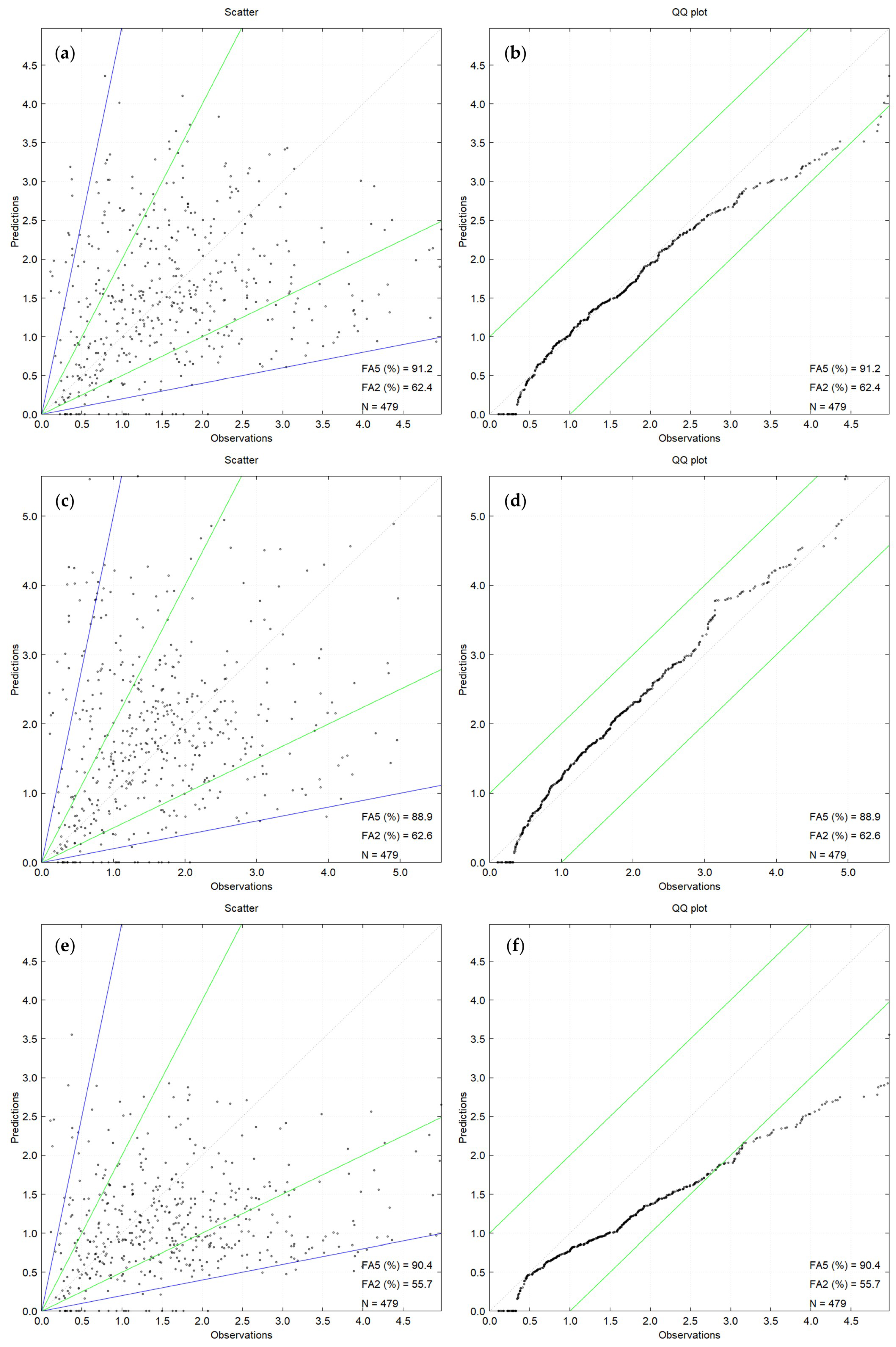
The scatter plots of predictions against observations are shown in Figure 1a for the three plume rise algorithms considered; they also report the FA2 and FA5 statistics. The predicted one-hour concentrations reported in the following figures have been obtained by calculating the concentrations three times during each hour (i.e., every 20 min) and then taking the arithmetic mean. The QQ plots are reported on the right panels of Figure 1.

It is observed that the regions of FA2 and FA5, delimited by the green and the blue lines of the scatter plots, respectively, are quite similar for the three plume rise algorithms: FA2 ranges from 55.7% (JJ + JJ) to 62.6% (JJ + RS), while FA5 ranges from 88.9% (JJ + RS) to 91.2% (WT). The QQ plots show three different behaviors depending on the plume rise algorithm. When the WT algorithm is used, LAPMOD has a tendency to underpredict for values of concentrations up to about 0.5 μg m⁻³, the distributions are in agreement for values in the range 0.5–2.3 μg m⁻³, then the model underpredicts for values greater than 2.3 μg m⁻³. When the JJ + RS algorithm is used, LAPMOD underpredicts for values smaller than 0.5 μg m⁻³ and overpredicts above such a value. Finally, when the JJ + JJ algorithm is used, the model always underpredicts the observed values. The QQ plot of the WT algorithm suggests proportionality between the distributions over the approximate range 1 to 3 μg m⁻³ (i.e., predictions and observations have similar mean and variance over this range). A similar proportionality over about the same range is observed for the JJ + RS algorithm, but shifted by about 0.2 μg m⁻³. It seems that, over this range, LAPMOD always overestimates the observations by about 0.2 μg m⁻³ when the JJ + RS algorithm is used.

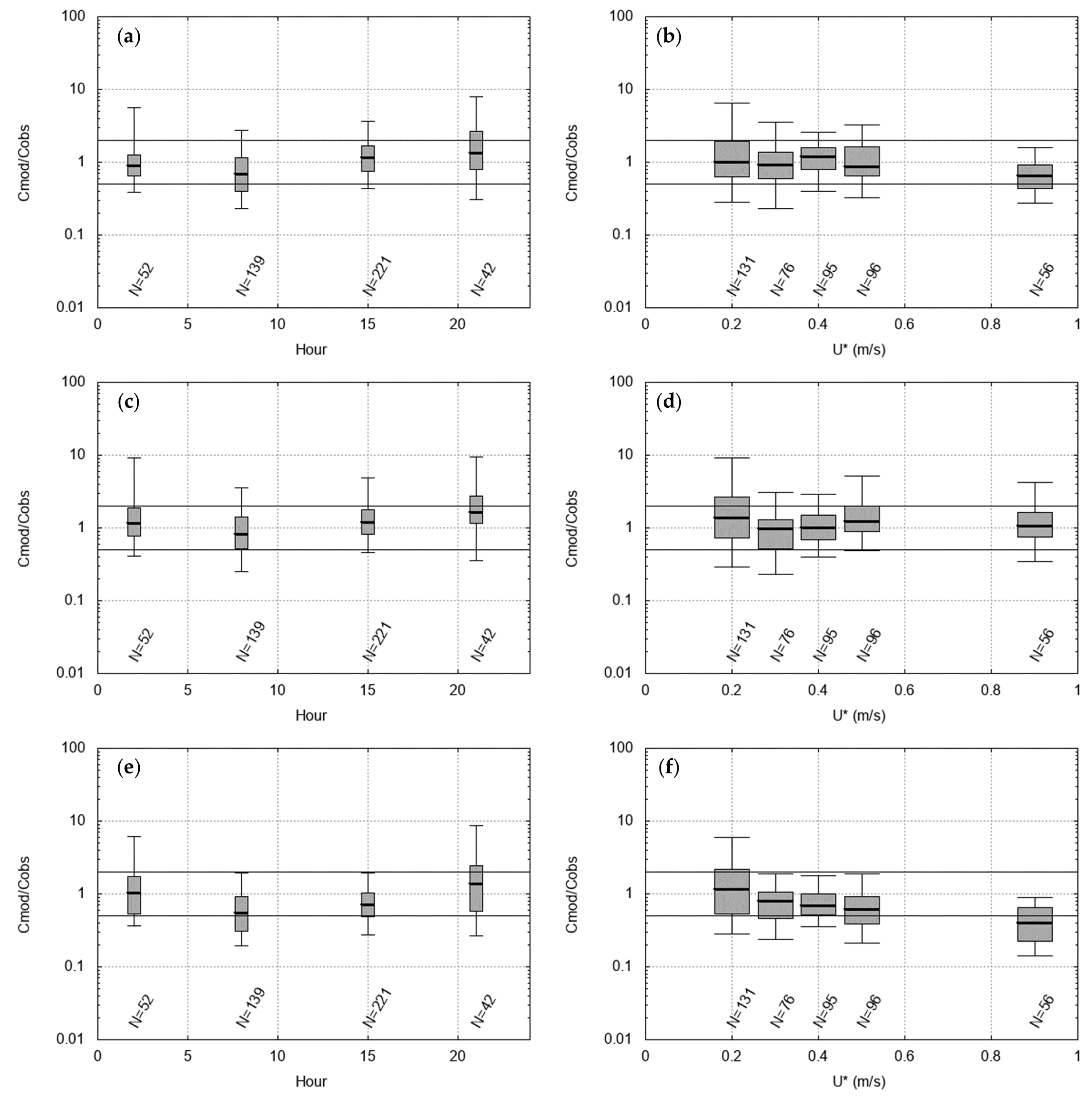
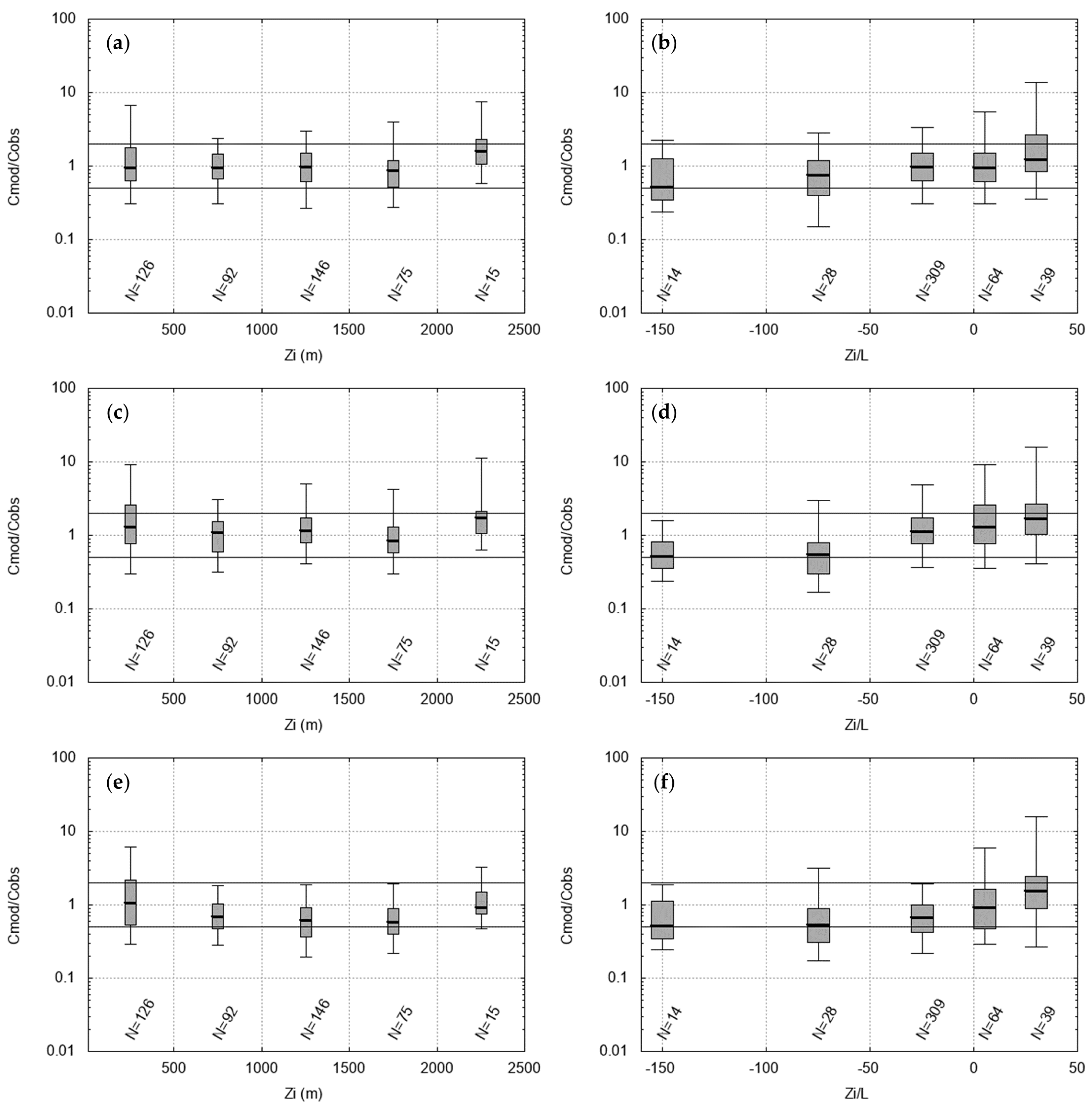
The residual box plots for Indianapolis best-quality data are reported in Figure 2 and Figure 3.

Remembering that the ratio between predictions and observations for a perfect model should always be 1, it is noticed that the LAPMOD results show that the medians of the ratios are almost always close to 1, and a significant proportion of the residuals falls within a factor of 2. The notable exception is the case with high friction velocity (>0.8 m s⁻¹) when the JJ + JJ plume rise algorithm is used. In these situations, all in the early afternoon, the observed wind speed is above 6 m s⁻¹, indicating slightly unstable to neutral stability conditions.

In Figure 2 and Figure 3, the data do not sum to 479 because there are situations where LAPMOD does not predict any concentration even though non-zero concentrations are measured. These situations are well visible on the X axis of the scatterplots (Figure 1a); specifically, for all three plume rise algorithms, there are always 25 combinations of hours and arcs in which this happens. This behavior is usually associated with strong stability conditions. For example, on 12 October 1985 (nocturnal release from 24:00 to 04:00), there are five situations where LAPMOD does not predict any concentration at ground level, while observations are in the range 0.72 μg m⁻³ to 1.77 μg m⁻³. 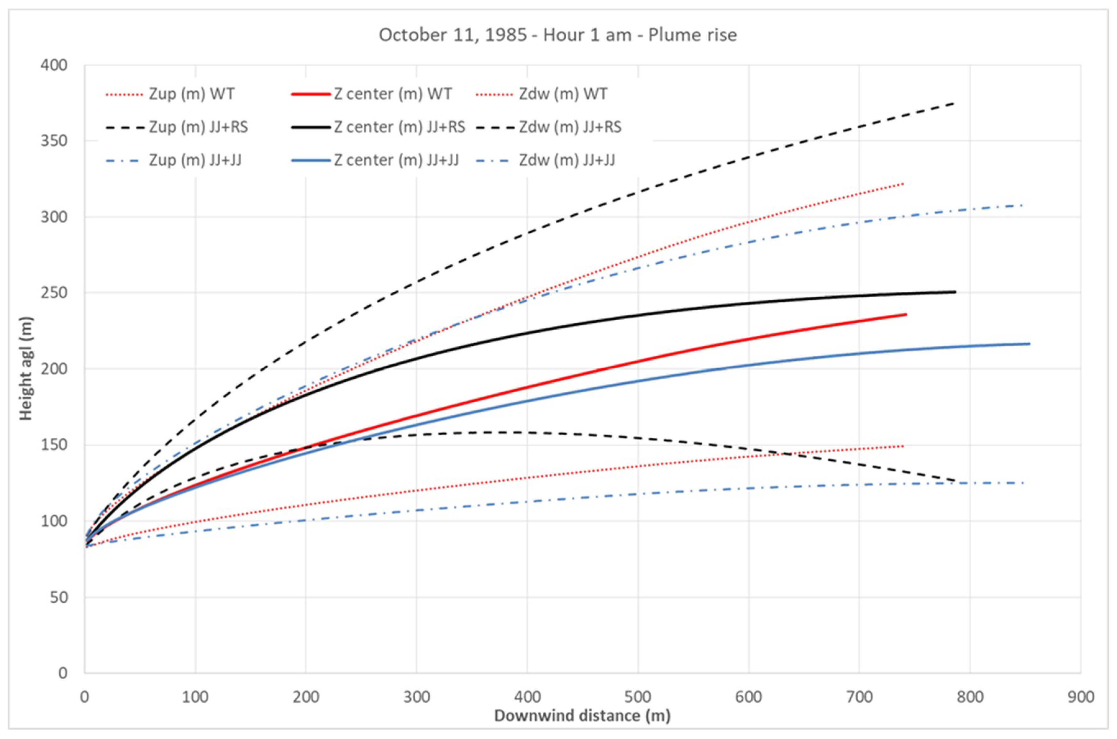In addition, on 11 October 1985, there are four situations where LAPMOD does not predict ground concentrations (all at 01:00), while observations range from 0.29 μg m⁻³ to 0.37 μg m⁻³. Similar situations are observed at 3 arcs at 01:00 on 1 October 1985, and three other times from 01:00 to 02:00 of 27 September 1985. The reason for this lack of modeling performance in cases of strong stability might be because the plume is too narrow aloft, and particles do not contribute to the ground level concentration. As an example, Figure 4 shows the plume shapes calculated by the three algorithms at 01:00 on 11 October 1985. At that hour the mixing height is 47 m and the concentrations observed at arcs from 1 km to 3 km are in the interval 0.29 μg m⁻³ to 0.37 μg m⁻³. Wind blows from the north with a speed of about 1.3 m s⁻¹, and the Monin–Obukhov length is 11.2 m, thus indicating stability. The thick solid lines in Figure 4 show the plume’s centerlines, while the thin lines represent the plume boundary calculated by adding and subtracting the plume radius to the plume centerline.

The three algorithms in this specific hour behave very similarly: the final rise distance is in the interval 740–850 m, and the plume centerline is in the range from 217 m (JJ + JJ) to 251 m (JJ + RS). This is the case of a plume directly emitted above the mixing layer (stack height 83.8 m, mixing height 47 m), with a plume induced turbulence that is strong close to the emission point and reduces to the weak turbulence level of a stable layer as the distance from the stack increases. Therefore, at least theoretically, the model behavior seems to be correct. However, the measurements indicate that the tracer concentrations were observed at ground level. For ground level tracer concentrations to be measured in this situation, it is likely that the stable plume aloft is affected by intermittent effects caused by mechanical turbulence. In other words, the wind speed fluctuates and, during occasional and very brief time periods, it can be much higher than the average wind speed. During these short time intervals, the higher wind speed creates mechanical turbulence and mixing that grabs some fraction of the plume and fumigates below. Similar behavior has also been observed by other authors. For example, Luhar and Hurley [24] reported that “in TAPM occasionally the plume does not mix down to the ground under nighttime stable conditions, while the observations show otherwise”. Additional investigation is needed in both the model algorithms and the meteorological data to reconcile these inconsistencies.

The LAPMOD results for Indianapolis have been compared against observations using the MVK [7] too.

Table 1. Performance statistics for the Indianapolis observations of best quality (Part 1).

Model	Mean	σ	Bias	NMSE	r	FB	FS	FA2
Observations	351.54	221.38	0.00	0.00	1.000	0.000	0.000	1.000
LAPMOD WT	327.60	189.87	23.94	0.56	0.256	0.071	0.077	0.624
LAPMOD JJ + RS	394.81	241.90	−43.28	0.61	0.230	−0.116	−0.044	0.626
LAPMOD JJ + JJ	238.88	137.20	112.65	0.82	0.189	0.382	0.235	0.557

and

Table 2. Performance statistics for the Indianapolis observations of best quality (Part 2).

Model	1st High	2nd High	FBfn	FBfp	MOEfn	MOEfp
Observations	1067.6	1064.1	-	-	-	-
LAPMOD WT	935.5	881.3	0.317	0.246	0.694	0.745
LAPMOD JJ + RS	1196.3	1187.7	0.232	0.347	0.754	0.672
LAPMOD JJ + JJ	762.9	627.9	0.525	0.144	0.559	0.822

show the performances of LAPMOD with different plume rise configurations against the measurements carried out at Indianapolis. Both observations and model predictions have been normalized by dividing the concentrations for the emission rate and multiplying by 1000.

The values of the robust higher concentration, RHC_R [23], are shown in

Table 3. Extreme statistics for the Indianapolis best-quality observations (μg m⁻³).

Extreme Statistics	Observations	LAPMOD WT	LAPMOD JJ + RS	LAPMOD JJ + JJ
Maximum concentration	5.0	4.4	5.6	3.6
Top Ten average	4.7	3.8	4.9	2.9
RHC11	5.5	4.4	5.7	3.2
RHC26	5.5	4.5	5.6	3.5

. For comparison purposes, another evaluation ([1], in their Table 2), reports for AERMOD 16216 with different input options values ranging from 4 to 5. Additionally, other authors [25] reported a ratio between modeled and observed RHC_R, with R = 26, equal to 1.18 for AERMOD and 1.30 for ISCST3. We observe in Table 3 that the same ratios for LAPMOD are within the interval from 0.63 (worst result when JJ + JJ is used) to 1.02 (best results when JJ + RS is used).

3.2. Kincaid SF₆

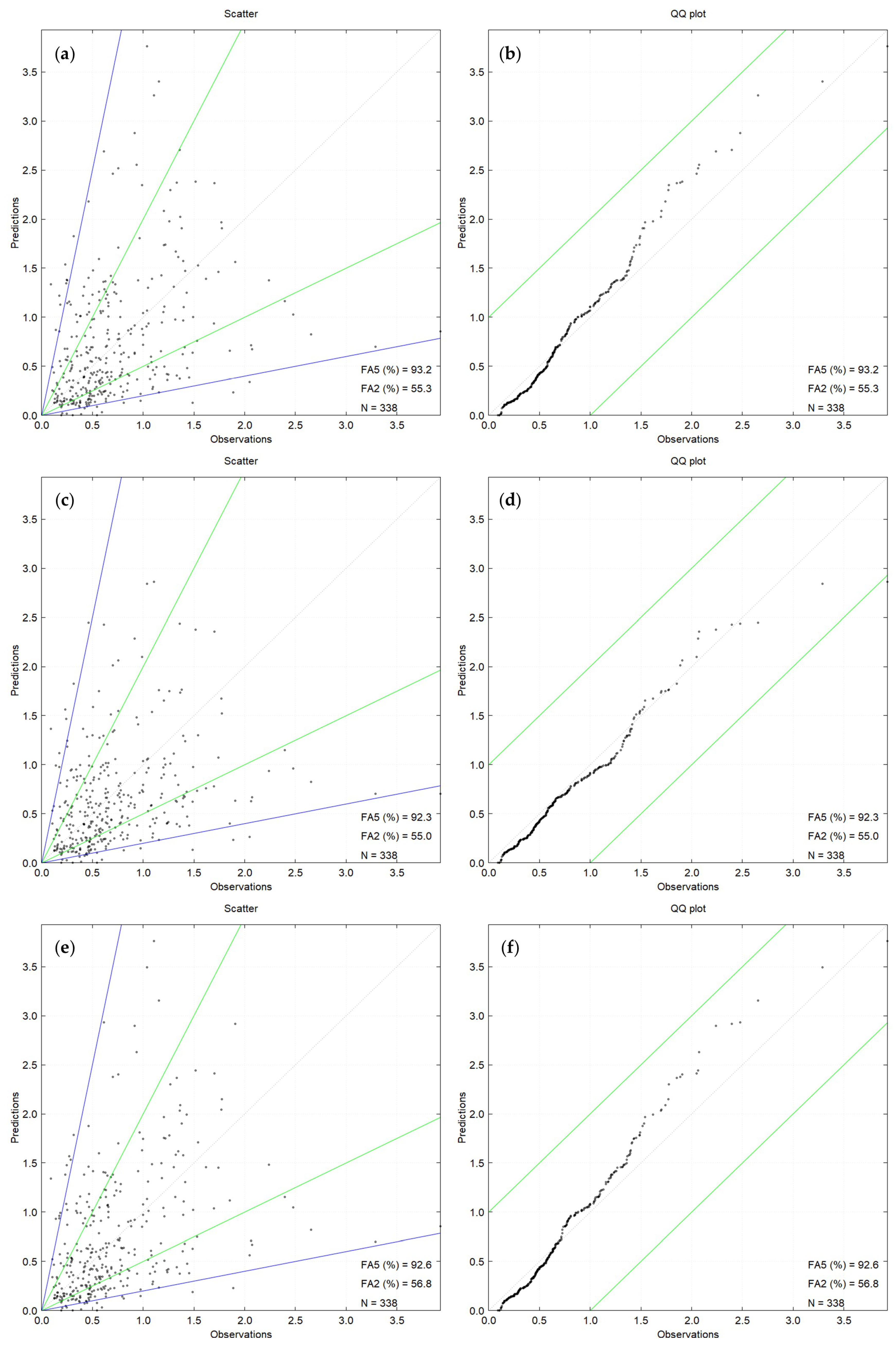
For the Kincaid SF₆ field experiment, LAPMOD was used with the same input variable configuration as the Indianapolis model run. A previous version of LAPMOD has already been validated against the Kincaid SF₆ data [4]; the validation is repeated here with a new version of the model and with the same input setting used for Indianapolis. As done for the Indianapolis dataset, only observations of best quality (338 values) were used for comparison with the model predictions. 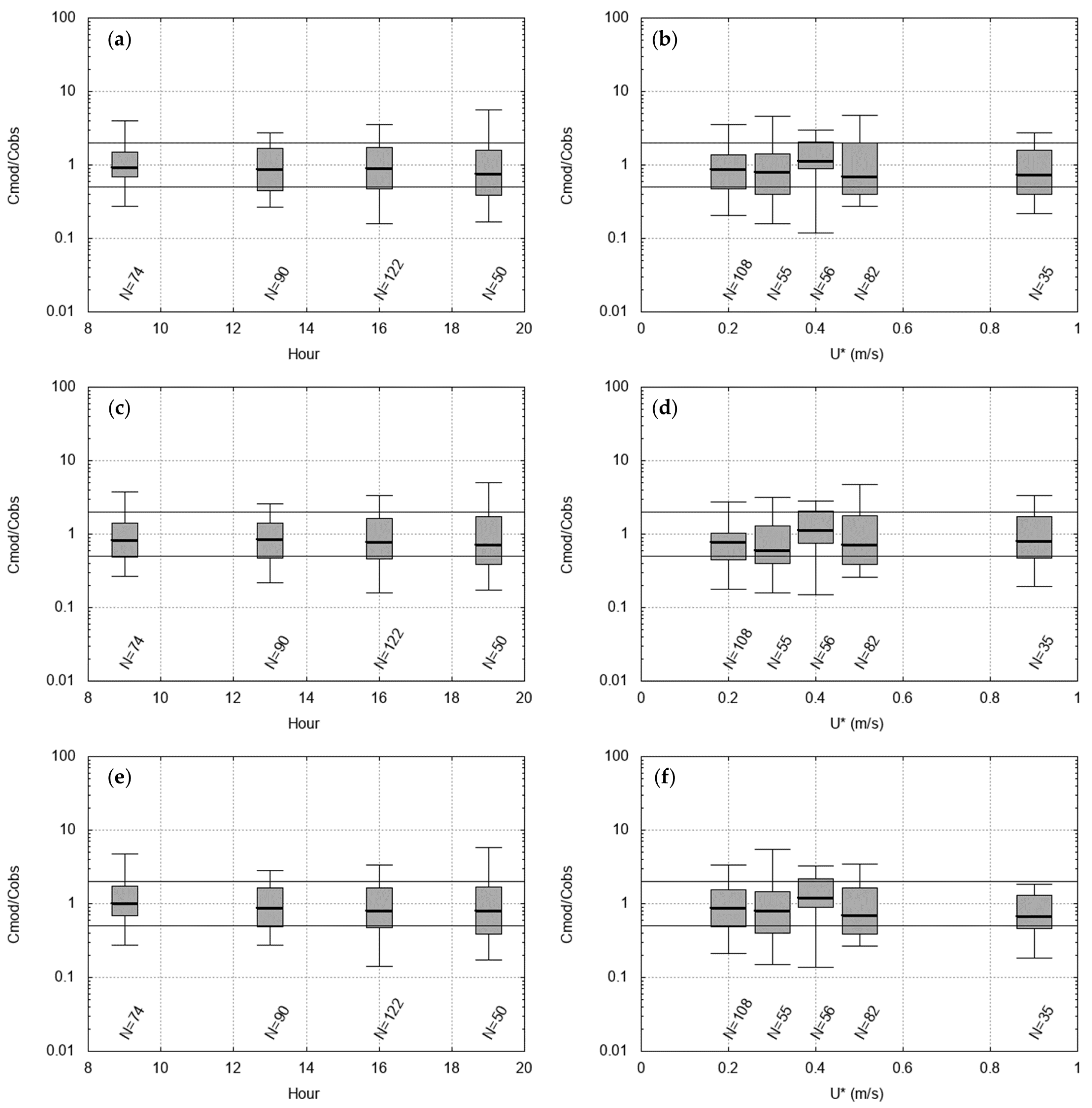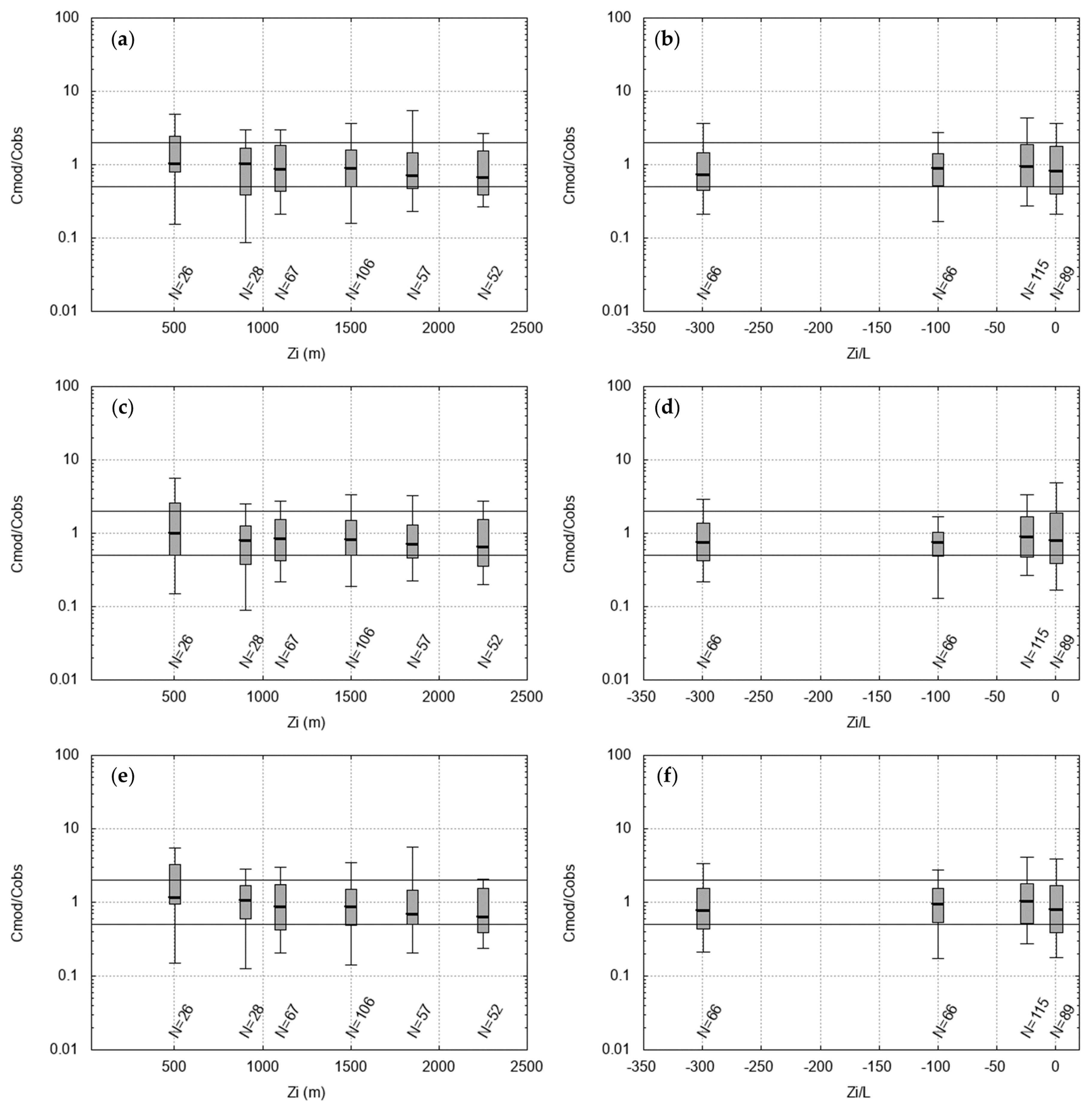The scatter plots of predictions against observations are shown in the left panel of Figure 5 for the three plume rise algorithm considered, while the QQ plots are shown in the right panel of the same figure. The residual box plots for Kincaid best-quality data are reported in Figure 6 and Figure 7; these plots have been created as described for the Indianapolis SF₆ data.

FA2 and FA5 are quite similar for the three plume rise algorithms: FA2 ranges from 55.0% (JJ + RS) to 56.8% (JJ + JJ), while FA5 ranges from 92.3% (JJ + RS) to 93.2% (WT). Concerning the QQ plot, it is observed that for the Kincaid SF₆ data the LAPMOD results are almost parallel to the x = y line up to about 1.5 μg m⁻³, 2 μg m⁻³ and 1.2 μg m⁻³, respectively, for algorithms WT, JJ + RS and JJ + JJ. A closer look to the curves shows that LAPMOD has a slight tendency to underpredict for values of concentrations up to about 0.7 μg m⁻³ when the WT and JJ + JJ algorithms are used, while above this value it overpredicts. When the JJ + RS plume rise algorithm is used, the overpredictions start at about 1.4 μg m⁻³. The residual box plots are always very similar, independently from the plume rise algorithm selected. The medians of the ratios are almost always close to 1, and a significant proportion of the residuals falls between a factor of 2.

The Kincaid observations of best quality and the LAPMOD predictions have been normalized by dividing them by the emission rate and multiplying by 1000. The MVK applied to the normalized data gives the results shown in

Table 4. Performance statistics of some dispersion models for the Kincaid SF₆ observations of best quality.

Model	Mean	σ	Bias	NMSE	r	FB	FS	FA2
Observations	54.34	40.25	0	0	1	0	0	1
LAPMOD WT	55.48	47.49	−1.14	0.8	0.381	−0.021	−0.083	0.553
LAPMOD JJ + RS	48.89	37.63	5.44	0.8	0.307	0.105	0.034	0.550
LAPMOD JJ + JJ	56.12	48.24	−1.78	0.76	0.417	−0.032	−0.090	0.568
HPDM *	44.84	38.55	9.5	0.75	0.441	0.192	0.043	0.565
OML *	47.45	45.48	6.89	1.24	0.146	0.135	−0.122	0.547
ADMS 3 *	51.7	34.7	2.7	0.6	0.45	0.05	0.15	0.67
AERMOD *	21.8	21.8	32.6	2.1	0.40	0.86	0.59	0.29
ISCST3 *	30	60	24.3	2.8	0.26	0.58	−0.39	0.28
NAME *	40.6	40.4	13.8	1.15	0.279	0.29	−0.005	0.615

* The performances of the other models appearing in table (HPDM, Earth Tech, USA; OML, NERI, Denmark; ADMS 3, CERC, UK; AERMOD, EPA, USA; ISCST3, EPA, USA; NAME, Met Office, UK) have been taken from [13].

. Additional LAPMOD statistics are reported in

Table 5. Performance statistics of LAPMOD for the Kincaid SF₆ observations of best quality.

Model.	1st High	2nd High	FBfn	FBfp	MOEfn	MOEfp
Observations	319.3	225.1	-	-	-	-
LAPMOD WT	276.6	259.3	0.304	0.324	0.693	0.679
LAPMOD JJ + RS	210.9	196.1	0.370	0.264	0.649	0.721
LAPMOD JJ + JJ	256.3	241.0	0.292	0.324	0.704	0.681

.

The statistics of extreme values for Kincaid SF₆, including the values of RHC_R with R = 11 and R = 26, are given in

Table 6. Extreme statistics for the Kincaid SF₆ best-quality observations (μg m⁻³).

Extreme Statistics	Observations	LAPMOD WT	LAPMOD JJ + RS	LAPMOD JJ + JJ	NAME *
Max concentration	3.93	3.76	2.86	3.76	3.93
Top Ten average	2.51	2.86	2.42	2.90	2.92
RHC11	3.61	3.73	3.14	3.84	4.33
RHC26	3.45	4.11	3.28	4.02	N/A

* The performances of the NAME model have been taken from [13].

. The statistics are reported for the observations, for LAPMOD with different plume rise algorithms, and, for comparison purposes, for the NAME model [13]. The maximum concentration is perfectly matched by NAME, while it overestimates RHC₁₁, as done by LAPMOD WT, which adopts the same plume rise algorithm. Other authors [25] reported a ratio between modeled and observed RHC_R equal to 0.77 for AERMOD and 0.68 for ISCST3 (with R = 26). We observe in Table 6 that the same ratios for LAPMOD are within the interval 0.95 (when JJ + RS is used) to 1.19 (when WT is used).

3.3. Kincaid SO₂

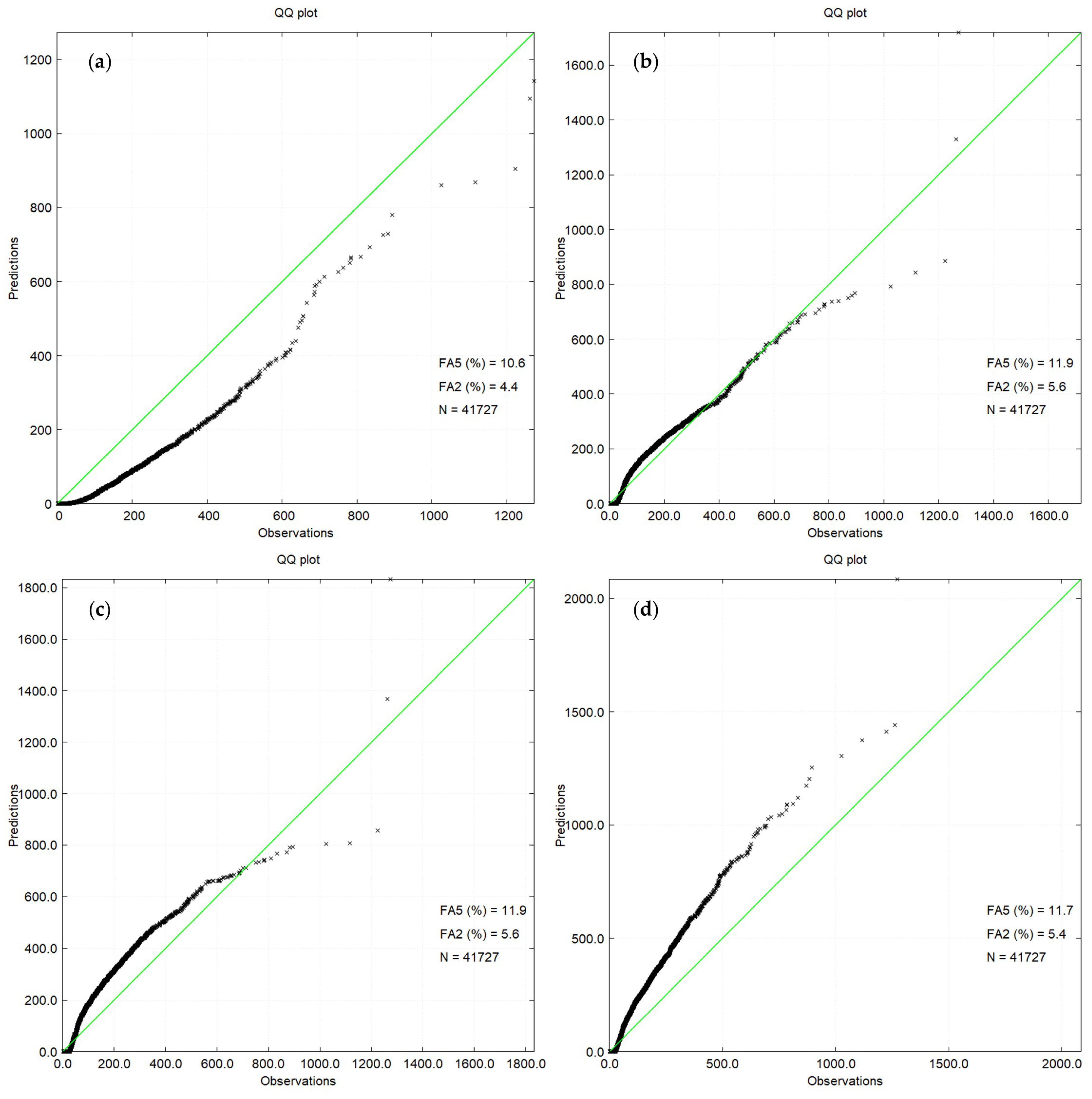
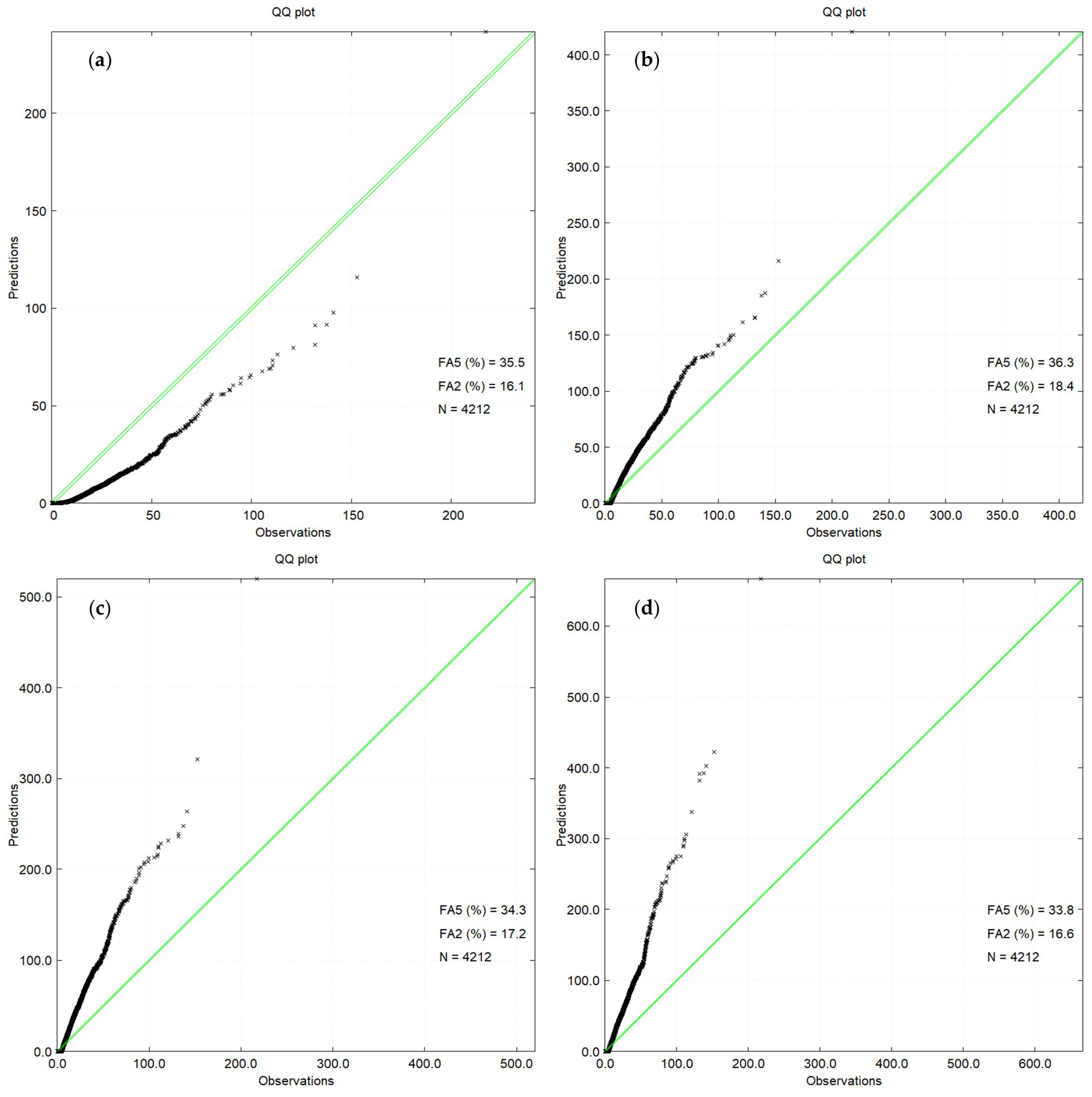
The QQ plot obtained for the one-hour average SO₂ concentration is shown in Figure 8 for AERMOD (upper left), LAPMOD WT (upper right), LAPMOD JJ + RS (bottom left) and LAPMOD JJ + JJ (bottom right). The AERMOD plots reported in this section have been created with the predictions distributed with the EPA’s model evaluation databases [20], which were obtained with a previous version of AERMOD (02222). AERMOD underestimates the one-hour concentrations while LAPMOD always overestimates them when the JJ + JJ plume rise algorithm is used. LAPMOD overestimates the observed concentration values up to about 700 μg m⁻³ and underestimates greater values when the JJ + RS algorithm is used, and it is in good agreement with the observations up to about 700 μg m⁻³ when the WT algorithm is used, while it underestimates for greater concentrations. The FA2 and FA5 values reported in Figure 8 are lower than those found for the SF₆ release because, as anticipated, the SO₂ release predictions and observations at each receptor have been paired in time. The values of these two statistics are similar for AERMOD and LAPMOD with different plume rise configurations.

The values of RHC and other statistics are reported in

Table 7. Statistics for the Kincaid SO₂ observations (μg m⁻³).

Statistics	Observations	AERMOD	LAPMOD WT	LAPMOD JJ + RS	LAPMOD JJ + JJ
Averages	9.1	2.9	11.9	16.2	18.2
Max values	1273.4	1489.9	1718.9	1832.5	2085.5
RHC26	1327.3	1329.0	1333.1	1439.8	1752.1

. The RHC₂₆ of AERMOD and LAPMOD WT are very close to the RHC₂₆ of the observations, confirming the ability to describe peak concentrations. On the contrary, LAPMOD JJ + RS and LAPMOD JJ + JJ tend to overestimate the observations.

The QQ plots obtained for the 24-h average SO₂ concentration are shown in Figure 9 for AERMOD (top left), LAPMOD WT (top right), LAPMOD JJ + RS (bottom left) and LAPMOD JJ + JJ (bottom right). AERMOD still underestimates the observations, while LAPMOD overestimates them with all the plume rise algorithms tested.

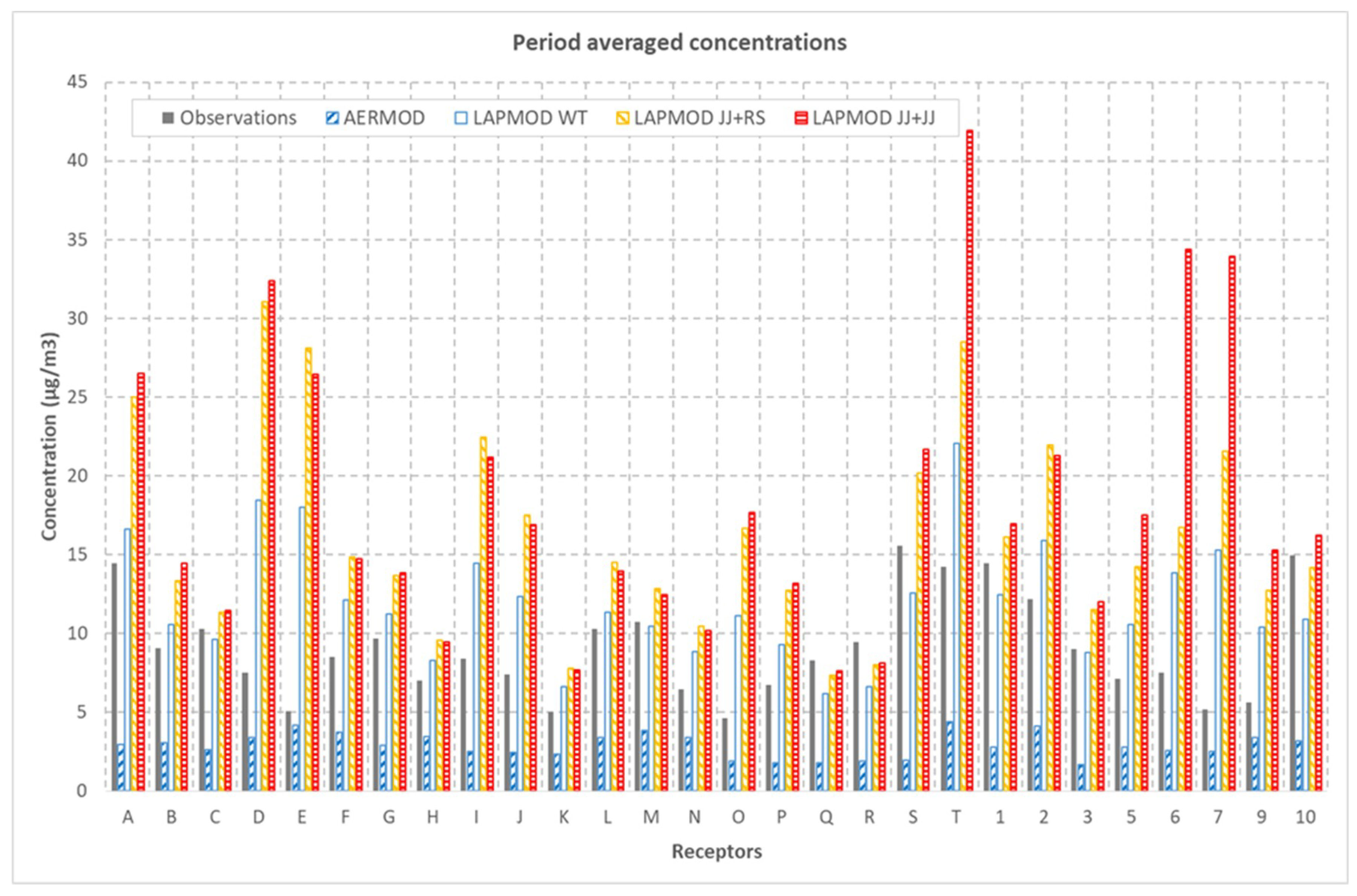
Figure 10 shows the period averaged concentrations at each receptor. After removing the values corresponding to zero SO₂ emission from the stack, the period-average at each receptor involve from 3023 to 4812 data. Generally, the LAPMOD average concentrations are in good agreement with the observations, with FA2 values ranging from 64.3% (JJ + JJ plume rise algorithm) to 85.7% (WT plume rise algorithm), and 10.7% for AERMOD. There are receptors at which LAPMOD greatly overestimates the observed concentrations, particularly at three receptors: T (the closest to the source at north), 6 (the closest to the source at south), and 7 (the closest to the source at south east). Considering also the behavior at other receptors, LAPMOD tends to overestimate average values close to the source.

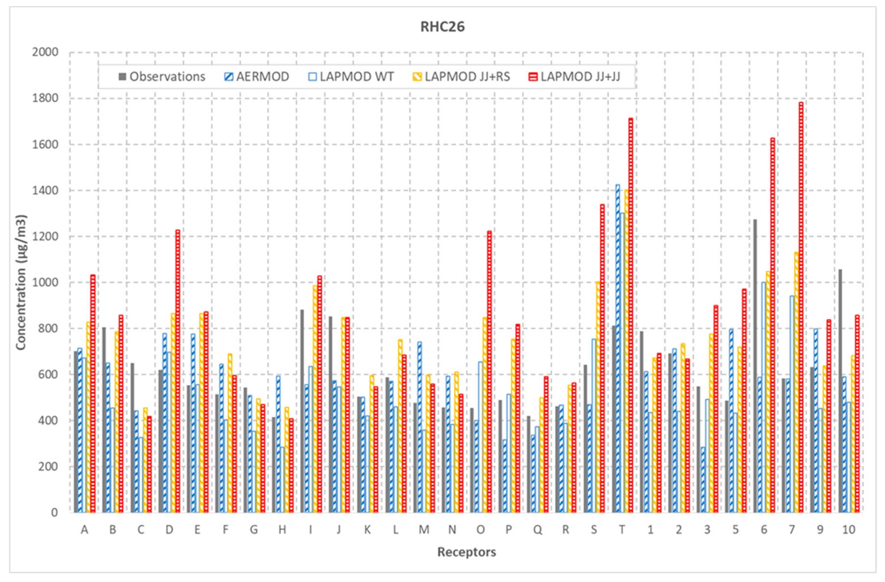
Figure 11 shows the RHC₂₆ values at each receptor. It is observed that considering the single receptors, instead of the whole one-hour concentration distribution independently from the position, the ability of LAPMOD to reproduce the peak concentrations improves. The maximum AERMOD RHC₂₆ (1424 μg m⁻³) is predicted at receptor T (the closest to the source at north), where observations give a value of 811 μg m⁻³ and LAPMOD WT a value of 1300 μg m⁻³. The maximum observed RHC₂₆ (1275 μg m⁻³) is at receptor 6 (the closest to the source at south), where AERMOD predicts 587 μg m⁻³, and LAPMOD WT 1000 μg m⁻³. For the other two plume rise algorithms, LAPMOD JJ + RS and JJ + JJ, the maximum observed RHC₂₆ values are 1046 μg m⁻³ and 1626 μg m⁻³, respectively. Receptors with a good agreement between observations and AERMOD are for example 7 and K.

4. Conclusions

This paper describes the numerical plume rise algorithms incorporated in the Lagrangian particle model LAPMOD [4] and their validation against experimental datasets. The LAPMOD model and its pre- and post-processors are freely distributed through the Enviroware’s website (https://www.enviroware.com/lapmod). The LAPMOD input files used to carry out the validations described in this paper are also available at: https://www.enviroware.com/lapmod/validations.html. The meteorological field input to LAPMOD can be prepared with the CALMET diagnostic meteorological model [5]. Thanks to its preprocessor LAPMET, the meteorological input can also be prepared starting from the AERMET output files. The LAPOST postprocessor allows the extraction of air quality statistics, concentration and deposition maps, and particle trajectories from the output binary files of LAPMOD.

Two plume rise algorithms have been incorporated in LAPMOD: Webster and Thomson [13] and Janicke and Janicke [12]. In this paper, we tested the WT algorithm and the JJ algorithm with two different entrainment mechanisms described in [12,16]. Therefore, we considered three different plume rise algorithms in total.

The WT and JJ plume rise formulations are comparable if the plume water content is not considered. The JJ algorithm has in its formulation the possibility to consider the effects of water, but in the datasets of Kincaid and Indianapolis, as in many others, the plume water content is unknown. Anyway, even for a dry plume, the JJ algorithm includes the effects of ambient humidity.

Apart from the plume rise algorithms, we defined the remaining LAPMOD input variables using the Indianapolis dataset, which was carried out in an urban environment. Then, we used the same input configuration for comparing the LAPMOD results against the Kincaid SF₆ and SO₂ datasets. Our goal was to verify that the model setting used for the Indianapolis data was also satisfactory for the Kincaid data to define a sort of default model configuration for future studies.

The results of LAPMOD with the different plume rise algorithms show that the Indianapolis data are best predicted when the JJ + RS plume rise algorithm is used. In such a case, FA2 is 62.6%, the QQ plot shows a good agreement between the observed and predicted data distributions, and good values for RHC_N are obtained, indicating a satisfactory capability to reproduce the highest concentration values as well. The results obtained with the WT algorithm are also good, while those relative to the JJ + JJ algorithm are characterized by a high value of FB (0.382). When the Kincaid SF₆ dataset is considered, the LAPMOD performances using the three plume rise algorithms are very similar. For example, the FA2 values are all within a narrow range (55.0–56.8%). Finally, the best LAPMOD results for Kincaid SO₂ have been obtained with the WT plume rise algorithm, both in terms of RHC₂₆ (1333 predicted versus 1327 observed) and in terms of period average concentration at each receptor.

Some performance evaluation criteria have been proposed [26,27] to define a “good” model. They require that at the same time the following three rules be observed:

• the fraction of predictions within a factor of two of observations is about 50% or greater (i.e., FA2 > 50%);
• the mean bias is within ±30% of the mean (i.e., roughly |FB| < 0.3 or 0.7 < geometric mean bias < 1.3); and
• the random scatter is about a factor of two to three of the mean (i.e., roughly NMSE < 1.5 or geometric variance < 4).

The above rules are not firm guidelines and it is necessary to consider all performance measures in making a decision concerning model acceptance. According to these criteria and to the results presented for Indianapolis and Kincaid SF₆, LAPMOD is a “good” model with all the three plume rise algorithms tested.

The above criteria do not hold for data paired in time and space, such as in the Kincaid SO₂ dataset where the performance statistics are lower.

Starting from the results obtained in this work, it seems that the model configuration used, with WT or JJ + RS plume rise algorithm, may be considered a good default for LAPMOD.

The LAPMOD computer running times are comparable with those of CALPUFF, and therefore LAPMOD is a cost-effective choice for air quality studies. Moreover, the structure of Lagrangian particle models is such that they can highly benefit from parallelization, for example distributing the particles’ movements to different processors.