The Street Air Warming Phenomenon in a High-Rise Compact City

Abstract

The street thermal environment is important for thermal comfort, urban climate and pollutant dispersion. A 24-h vehicle traverse study was conducted over the Kowloon Peninsula of Hong Kong in summer, with each measurement period consisting of 2–3 full days. The data covered a total of 158 loops in 198 h along the route on sunny days. The measured data were averaged by three methods (direct average, FFT filter and interpolated by the piecewise cubic Hermite interpolation). The average street air temperatures were found to be 1–3 °C higher than those recorded at nearby fixed weather stations. The street warming phenomenon observed in the study has substantial implications as usually urban heat island (UHI) intensity is estimated from measurement at fixed weather stations, and therefore the UHI intensity in the built areas of the city may have been underestimated. This significant difference is of interest for studies on outdoor air temperature, thermal comfort, urban environment and pollutant dispersion. The differences were simulated by an improved one-dimensional temperature model (ZERO-CAT) using different urban morphology parameters. The model can correct the underestimation of street air temperature. Further sensitivity studies show that the building arrangement in the daytime and nighttime plays different roles for air temperature in the street. City designers can choose different parameters based on their purpose.

1. Introduction

Streets are where life, traffic, and commercial activities mingle together in large cities. Streets represent the immediate thermal environment for buildings, and the heat, moisture, wind, and so on emitted from buildings also change the environment in the street. The street thermal environment determines the thermal comfort of citizens, especially important for outdoor workers [1,2,3] and, as climate is warming globally, cities such as Hong Kong will experience greater stress. Accurate information about the street thermal environment is also important for the analysis of urban climate and pollutant dispersion. Being high-rise and compact, Hong Kong has had an urban warming rate of 2 °C over the last 100 years, which is much higher than the global warming rate of 0.7 °C over the same period [4].

The outdoor air temperature is a main factor to determine physiological equivalent temperature, which is important for evaluation of thermal comfort [5]. However, obtaining accurate air temperature in the street is not easy. It is known that weather station data depend on the location of the station and its surroundings. For stations installed in the urban canopy layer, the radius of influence is usually below 500 m [6]. Since weather stations are usually surrounded by open and/or green areas, whether data from weather stations alone can accurately represent air temperature within high-rise city is still an unanswered question. Installing fixed station in the streets and using vehicle traverse methods are two other options, but the former may not be suitable everywhere due to logistical restrictions.

Vehicle traverse methods have been used to measure air temperatures in cities. The monitored air temperature data from traverse experiments have been used to determine air temperatures over a whole city [7,8,9,10], but most of these field studies were carried out in cities where the building arrangement is sparse such as Singapore and Utrecht [7,11], and few studies [12] have been carried out in high-rise cities, such as Tokyo and Hong Kong. Pioneering work on street canyons [13,14] has led to an improved understanding of heat and turbulent transport in street canyons [15,16,17,18,19,20,21]. Field studies of thermal and airflow characteristics in streets have been carried out [22,23]. Simple models have also been developed to understand changes in air temperature in street canyons [24]. However, most studies of street canyons and air temperature were focused on isolated canyons. Very few studies have focused on the average air temperatures in street canyons over a large part of a city, particularly in high-rise compact cities.

Thermal imagery and thermal remote sensing techniques are other methods to quantify land surface temperature and near surface air temperature to monitor and study the urban heat island effect [25,26,27]. Studies have found that both the urban morphology, which shows different arrangement of building clusters and the surface (impervious surface or vegetation cover) play important roles for surface and air temperature in an urban environment [5,28]. This method has also been also used in Hong Kong, where Fung et al. [29] and Nichol et al. [30] analyzed surface temperature distributions on a winter night. However, the disadvantage of remote sensing is that the air temperature must be derived from surface temperature. Since full diurnal cycles of air and surface temperature have pronounced hysteresis effects at local scale, the derivation of the air temperature from surfaces may not be accurate at local scale [31].

Some local studies in Hong Kong have focused on deep street canyons [32,33] using computational fluid dynamics (CFD) simulations, but consideration of the thermal environment is limited. Street air temperatures are measured at the neighborhood-scale [34,35,36], but most studies focus on the specific time of day, such as noon, afternoon, or nighttime. However, only a few studies have considered the variation of the full diurnal cycle of temperature, which is important to further understand the mechanisms of temperature variation.

Furthermore, numerical models for street temperature have usually focused on local scale, and the simple mesoscale model which includes the effect within streets is limited. Silva et al. [37] developed a zero-dimensional mesoscale model to evaluate energy balance including simplified complex urban geometry. However, in this model, the urban surface temperature and air temperature were set to uniform, while they are known as very different [38]. Yang et al. [39] improved the model by developing separated characteristic temperatures for urban air and urban surfaces. However, flow pattern in compact street areas are different from open areas or the ideal city. Therefore, the model should be improved if we want to improve our understanding of the impact of urban morphology on urban air temperature, especially street temperatures.

In streets of the compact high-rise city, the low ventilation rate [40] leads to high temperature, while the low sky view factor causes low incoming solar radiation [39,41]. The interaction of such factors is complicated and still not fully resolved. The purpose of this paper is to study the diurnal air temperature profile and its impact in street canyons of Hong Kong using both traverse data and an improved urban canopy layer temperature model based on the ZERO-CAT model [39], in the attempt to accurately reproduce street air temperature. This should allow sensitivity studies of different factors of urban morphology based on the model to be analyzed, thereby helping designers understand the influence of these factors on thermal comfort.

2. Experiments

2.1. Experimental Area

The experiment was conducted in the southern part of Kowloon Peninsula (Figure 1), one of the core urban areas in Hong Kong. Due to high population density [42], the study area comprises narrow streets and very tall buildings (Figure 1), making it a compact, high-rise area.

2.2. Designed Traverse Route

The traverse route was designed to measure the air temperature in the streets in the chosen experimental area, which is the Kowloon Peninsula area of the city (Figure 2 top). The experiment was conducted along roads forming a loop that represent the main character of the city center, including main roads and small alleys, the CBD area, and green areas (Figure 2 bottom). The speed of the vehicle was approximately 30 km/h, and both the starting and ending locations were at the Hong Kong Polytechnic University, indicated by a blue triangle in Figure 2 (top). The route consisted of an anticlockwise loop, and most loops were completed within an hour. The elevation gradient of the route is less than 50 m, which is small enough to ignore the temperature–altitude correction [43]. The designed route also passed by the area near the two fixed weather stations operated by Hong Kong Observatory: the Hong Kong Observatory (HKO) station and King’s Park (KP) station (Figure 2 top). Both stations are located in the urban area and the temperature obtained from HKO station is usually adopted to represent the city temperature in Hong Kong [4].

2.3. Instrumentation

The data were collected along the designated route by an instrumented vehicle. Instruments included three air temperature sensors and two global positioning system (GPS) sensors (eTrex, Garmin, Olathe, KS, USA). The GPSs, with recording frequency of 1 s, were attached to the vehicle. Three temperature sensors were located on the vehicle roof, the height of which is about 2 m (Figure 3). The top of vehicle roof is a common location for measuring temperature in traverse experiments [7,10,11,44]. The air temperature sensors are marked by the black circle in Figure 3. A two-layer well-insulated and mechanically-ventilated plastic tube with aluminum foil was used as a cover to shield solar radiation, an improvement from the tube used in several studies. The K type thermocouple probes (Model EW-08505-86, Cole-Parmer, Vernon Hills, IL, USA) was placed in the middle of the tube and recorded every 4 s by a thermometer data logger (Extech-HD 200, Extech Instruments, Nashua, NH, USA) [11,12]. The record frequency was higher than that of Wong et al. [11]. The temperature record and the GPS record were matched to local time, which was calibrated in each instrument and experiment.

The probes were first calibrated by plotting the thermocouple’s voltage–temperature curve. The tube was aspirated at a rate of 3.5 m/s by a fan at one end of the tube. All tubes were installed in a single direction to ensure air flow from the front of the vehicle. The data were averaged among three temperature sensors located on the vehicle roof to minimize the effect of the possible exhaust gas plumes from other vehicles in front and on either side of the experiment vehicle. The three tubes on the vehicle roof were at equal distance (around 500 mm) to one another. The tube was also tested for 24 h at a location 15 m from the KP station. The average difference between the measured air temperatures of the two sensors was less than 0.1 °C for non-rainy days, as shown in Figure A1, Appendix A. Before each experiment, all sensors were calibrated and the GPSs were compared with one another.

2.4. Data Analysis and Validation

The field measurements were conducted from August to September 2012. A total of 158 vehicle traverse loops was conducted in a total of nine days, with each period consisting of 2–3 full days. Sunny days with low background wind speed were selected, to represent the typical UHI situation.

Table 1. List of the experiment periods and locations.

Reference Period (P)	Start Time 1 of Measurement	End Time 1 of Measurement	Hours (days)	Loops
Period1 (P1)	12:00, 20 August	16:00, 22 August	52 (2+)	39
Period2 (P2)	12:00, 9 September	16:00, 12 September	76 (3+)	62
Period3 (P3)	18:00, 15 September	16:00, 18 September	70 (3−)	57

¹ Local time.

presents details of each measurement. General weather information is provided in

Table A1. Weather conditions during the measurement periods at three HKO weather stations.

HKO Stations (see Figure 1)		HKO (Representing an Urban Area)					TYW (Representing a Rural Area)		WGL (Representing the Rural Wind)
Period	Date	Max Temp (°C)	Ave Temp (°C)	Min Temp (°C)	Ave RH (%)	Ave Cloud (%)	Ave Temp (°C)	Ave RH (%)	Prevailing Wind Direction (degrees)	MeanWind Speed (km/h)
P1 (summer)	20 August 2012	32.9	29.5	27.5	76	51	27.5	87	210	11.7
	21 August 2012	31.6	29.1	27.8	79	63	26.7	92	230	11.5
	22 August 2012	28.9	28.0	26.6	80	80	26.4	91	280	10.6
P2 (summer)	9 September 2012	32.7	29.5	27.7	78	44	27.2	87	120	7.7
	10 September 2012	31.8	29.3	27.7	77	59	27.4	86	180	8.8
	11 September 2012	33.6	29.9	27.8	75	54	27.4	85	120	14.5
	12 September 2012	33.2	29.8	27.9	77	53	27	88	120	13.0
P3 (summer)	15 September 2012	28.9	26.5	24.2	65	85	25.4	66	20	23.8
	16 September 2012	29.5	27.0	24.3	63	23	25.1	70	20	13.3
	17 September 2012	30.8	27.0	23.6	54	4	24.6	63	10	15.7
	18 September 2012	30.4	27.4	25.3	59	68	23.7	78	30	10.1

, Appendix B. Due to a small bias of the GPS coordinate during the experiment, we used the “cell” (as defined above) to represent the location. The study area was sub-divided into 100 × 100 m² cells, as shown in Figure 4, with the choice of the length scale 100 m determined from the temperature recording frequency, vehicle speed and the responding time of temperature sensors. Data when the car speed was zero were deleted to avoid the influence of traffic jams. The remaining temperatures in each cell were averaged. For further data analysis, only the data of a whole day (0:00–23:59) were used for Fast Fourier transformation (FFT). Therefore, three experiments were conducted to collect adequate data samples.

3. Numerical Simulation

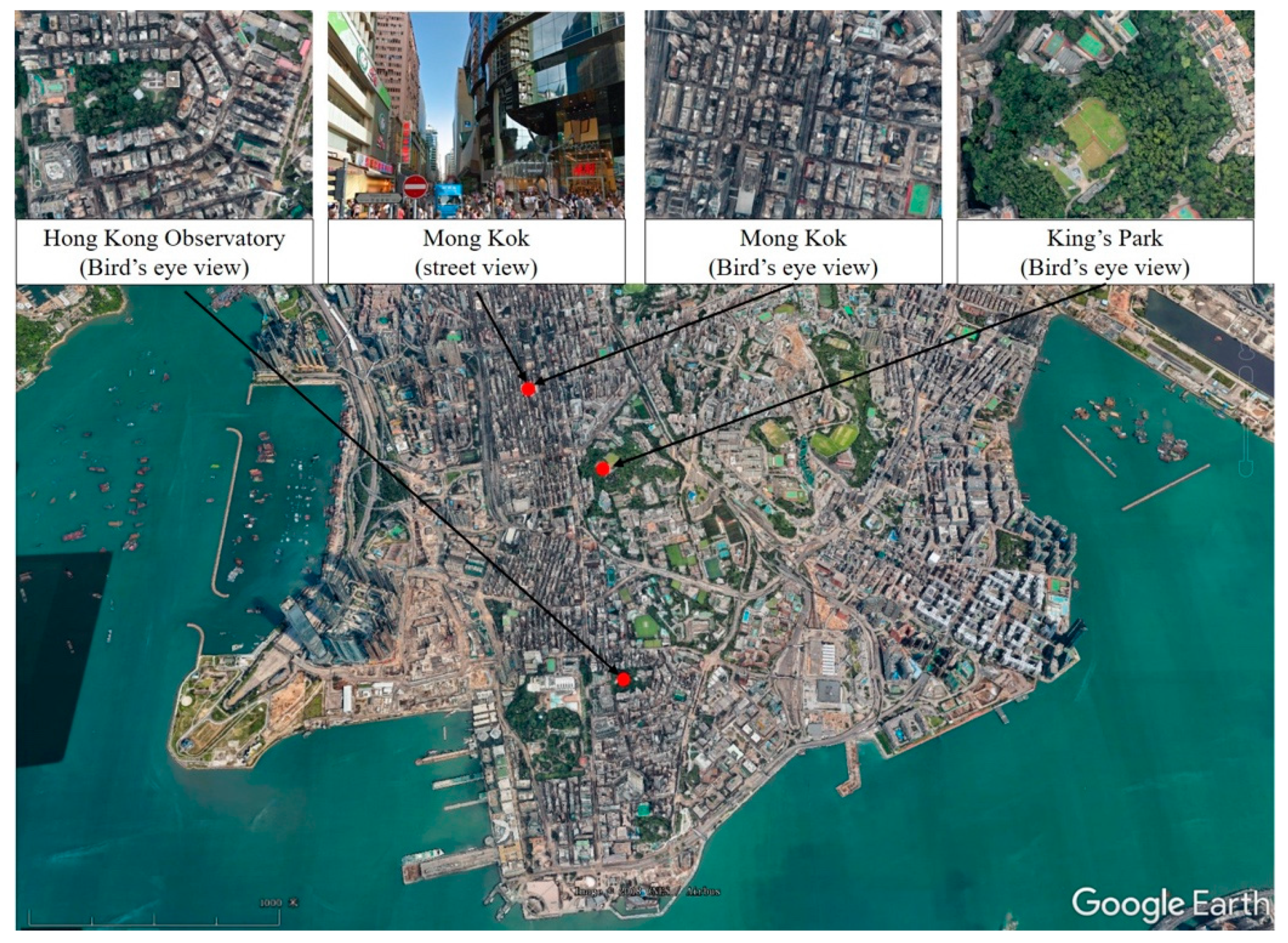
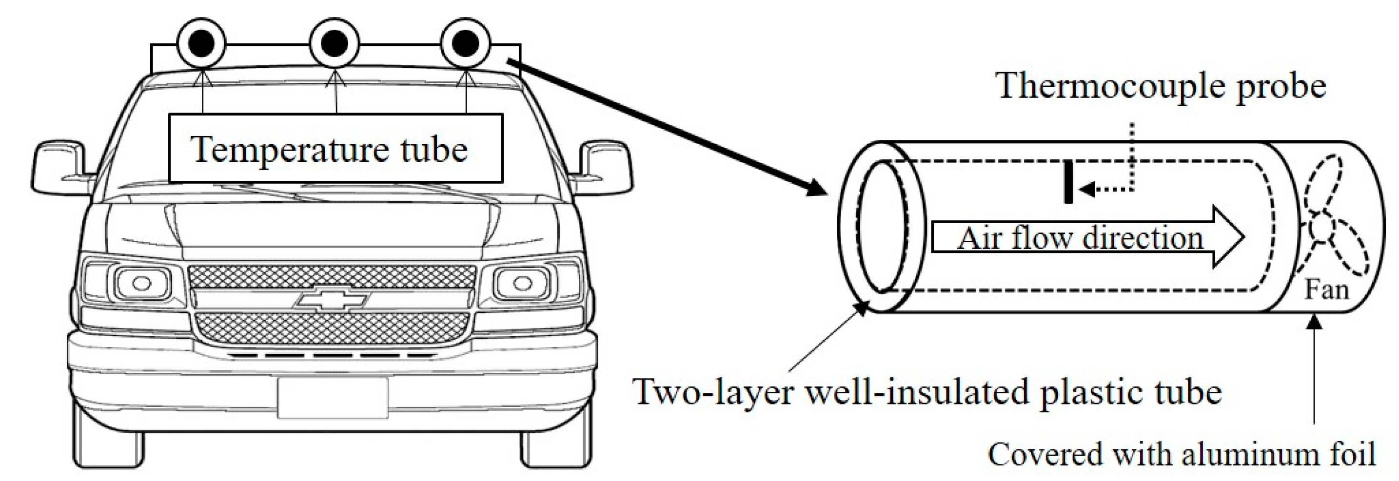
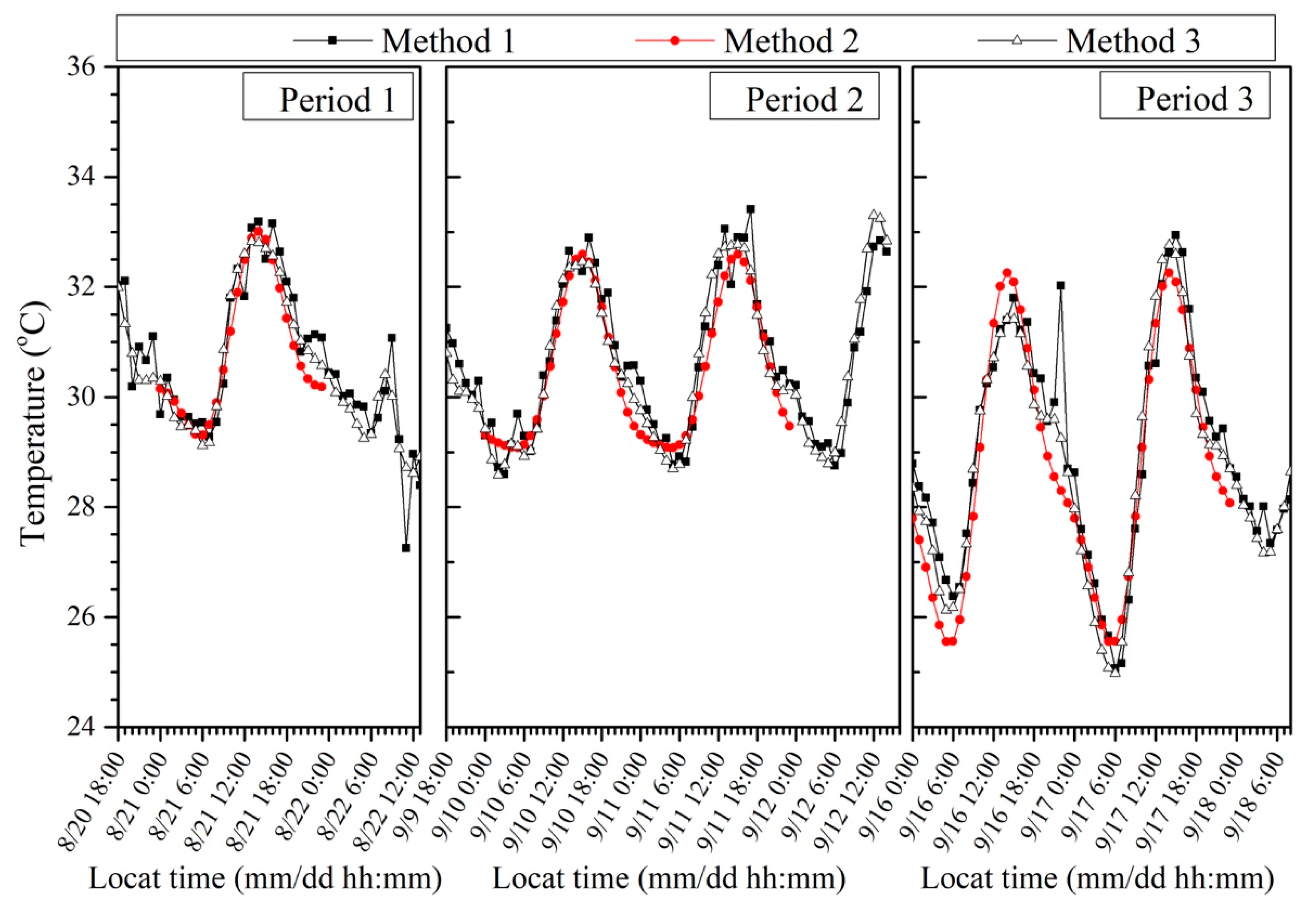
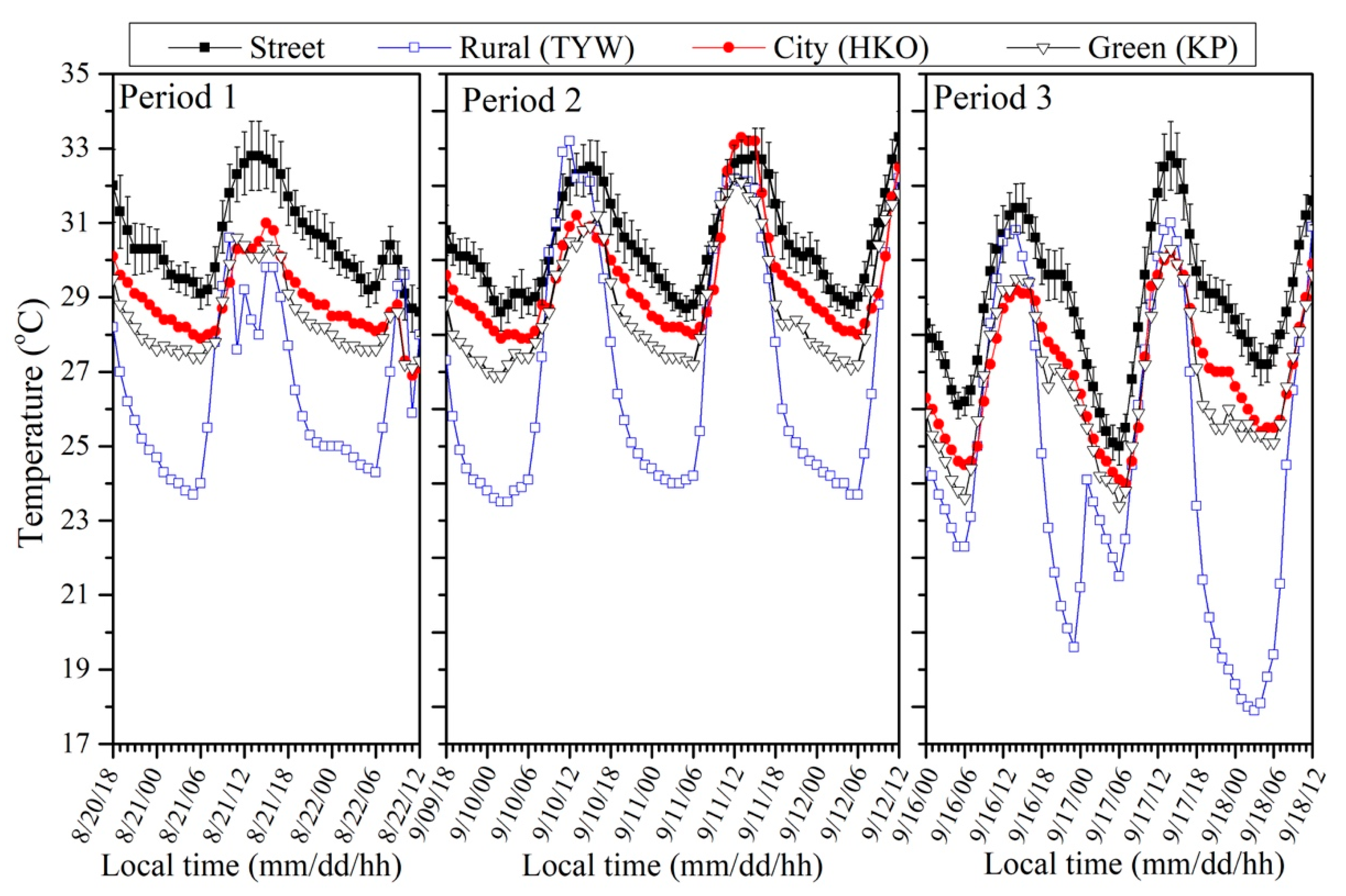
3.1. Model Description

Yang et al. [39] developed a model to determine the air temperature in the city, which is referred to as zero-dimensional City Air Temperature (zero-CAT) model. However, the ventilation rate and the anthropogenic heat in the zero-CAT model is not applicable for the street, especially in a compact high-rise city such as Hong Kong. The model is improved in this section.

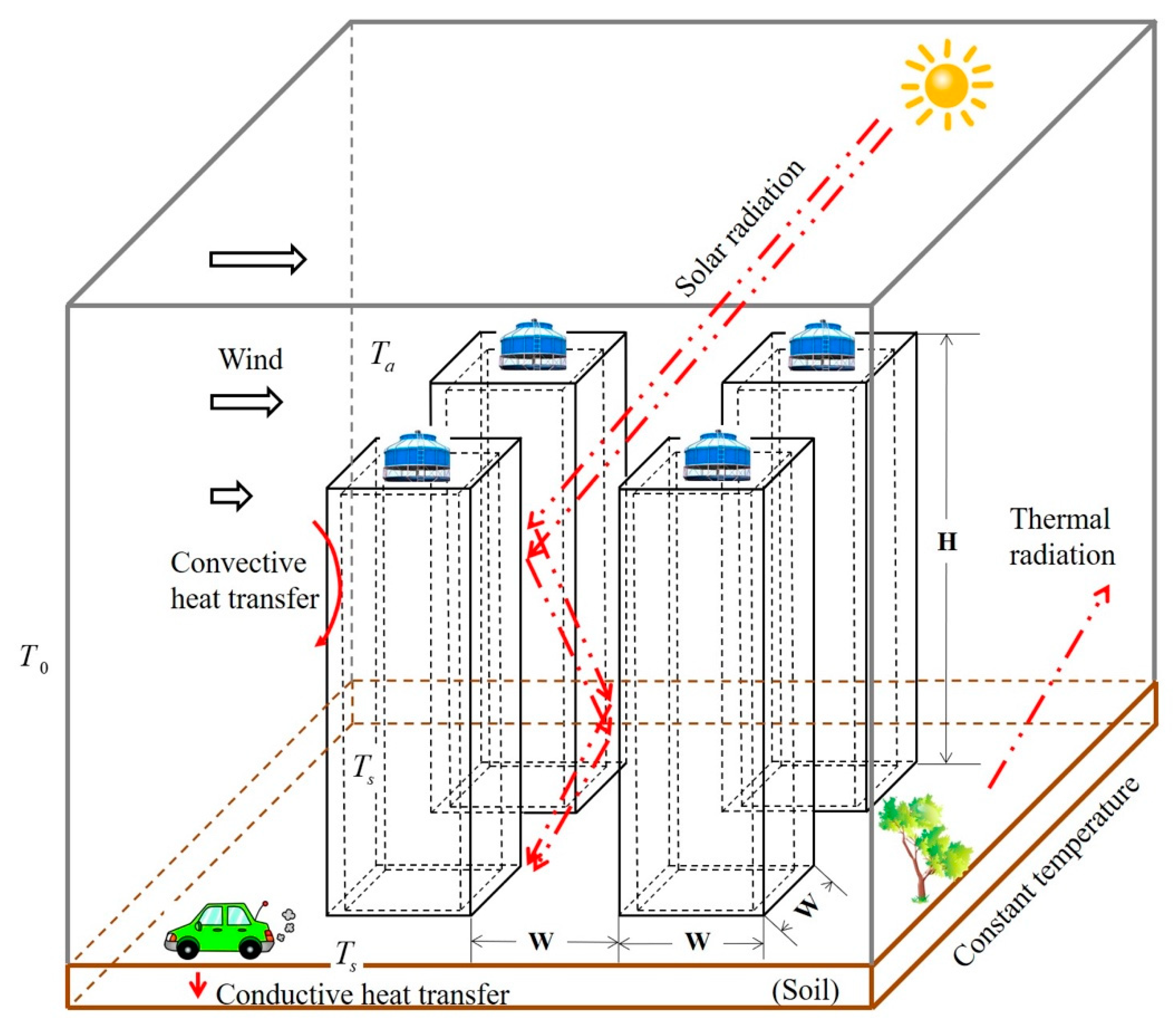
The original model is based on the zero-dimensional mesoscale model to determine urban surface temperature originally developed by Silva et al. [37]. The zero-CAT model cataloged the urban fabric into different types and linked the air and surface temperature together through an analytical solution of urban air temperature. 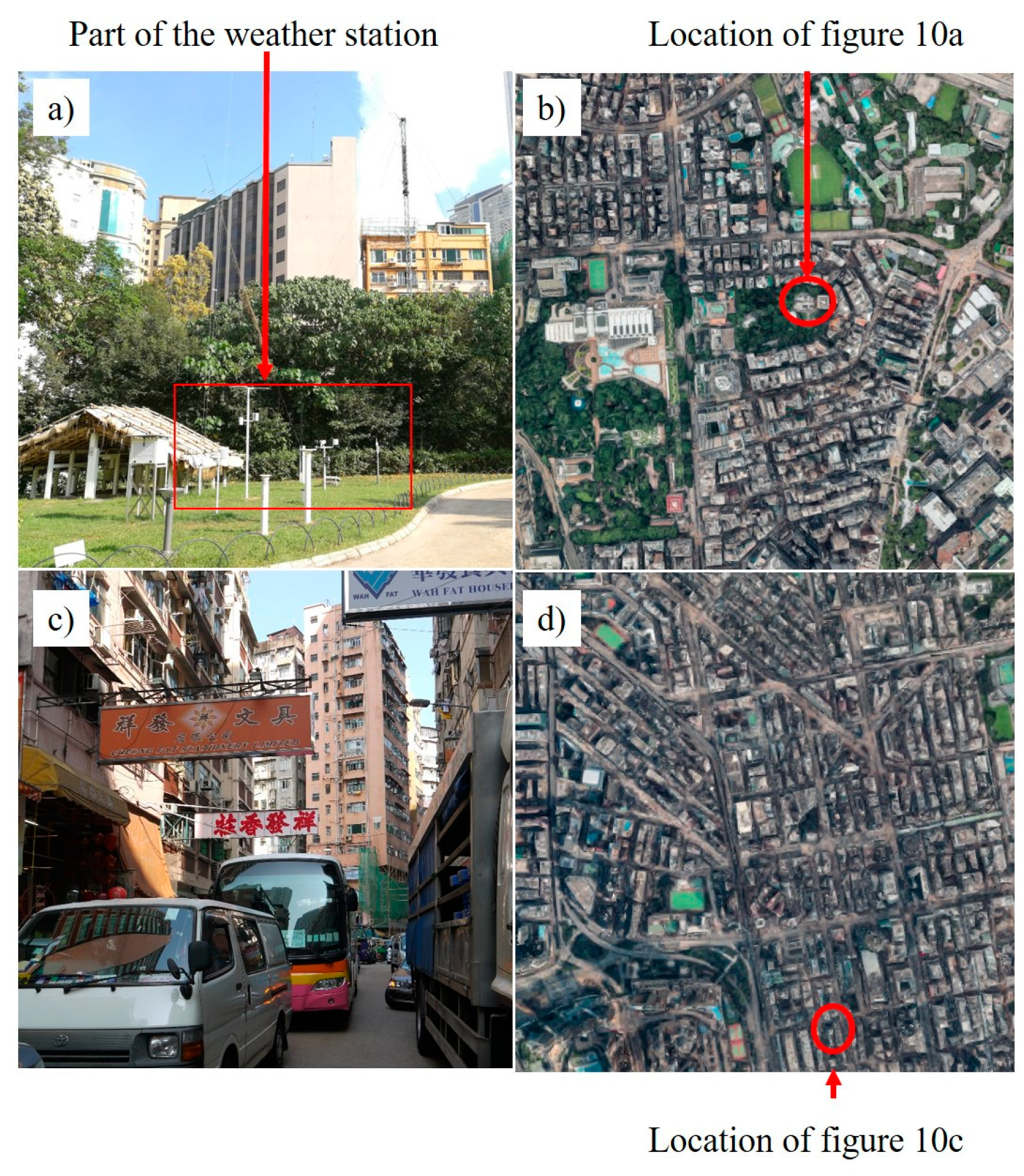Two assumptions are made to simplify the city to a simple and ideal control volume for the zero-CAT model (Figure 5).

(1)

The city is composed of buildings, streets, plants, and vehicles. The underlying surface is concrete with uniform distribution for the city area. The plan area ($A_p$) includes the area of the green zone ($A_g$), such as plants and parks; the area of the streets covered by pavement ($A_c$); and the building roof area ($A_r$). The total area of the surfaces ($A_t$) in the control volume includes both the plan area ($A_p$) and the surface area of the buildings ($A_b$), including wall surfaces and the roof of buildings. The relation of the terms is shown in Equations (1) and (2).

$$A_t=A_p+A_b$$

(1)

$$A_p=A_g+A_c+A_r$$

(2)

The plan area coverage ratio ${\lambda }_p$, calculated by Equation (3), represents the density of the city. The frontal area ratio ${\lambda }_f$, is calculated by the area of the wall of the building which facing the inflow ($A_f$) and the total plan area, as shown in Equation (4) [45]

$${\lambda }_p=A_r/A_p$$

(3)

$${\lambda }_f=A_f/A_p$$

(4)

(2)

The airflow is assumed to be fully mixed, so the air temperature ($T_a$) distribution in the domain is uniform. The temperature distribution in the thermal mass except for the underlying surface is also assumed to be uniform, and the surface temperature is referred to as $T_s$. The rural air temperature $T_0$ is also uniform. The air temperature from the representative rural station was used as the temperature of the incoming air [39].

With all assumptions, two heat balance equations are used in the city, one for the outdoor air and one for the surface temperature. The balance equation of the urban air is

$${\rho }_{air}{c}_{p}q\left(T_0-T_a\right)+h_{sh}{A}_t\left(T_s-T_a\right)+q_{anth}{A}_p=0$$

(5)

where ${\rho }_{air}$ is the density of the air, $c_p$ is the heat capacity of the air, $q$ is the ventilation rate, $h_{sh}$ is the sensible heat flux transfer coefficient, and $q_{anth}$ is the anthropogenic heat.

The surface energy balance equation is:

$$mc\frac{d{T}_s}{dt}=A_p\left(1-\alpha \right)q_{sol}-A_g{q}_{cond,g}-A_c{q}_{cond,c}-A_b{q}_{cond,b}-A_g{q}_{evp}-A_t{q}_{conv}-A_p{q}_{rad}$$

(6)

where $mc$ is the thermal mass of the urban area. The terms on the right side are the different energy terms gained in the control volume. The term $A_p\left(1-\alpha \right)q_{sol}$ is the solar radiation absorbed by the urban fabric, $q_{sol}$ is the solar radiation, $\alpha$ is the albedo of the volume, and $A_g{q}_{cond,g}$ and $A_c{q}_{cond,c}$ are the conductive heat flux into vegetated areas and roads, respectively. $A_i{q}_{cond,i}$ is calculated by $A_i{k}_f\frac{T_s-T_{i\_sub}}{\Delta x_f}$, where $k_f$ is the conductivity of the surface type $f$, and $\Delta x_f$ is the representative depth in which the diurnal temperature variation is ignored. $T_{f\_sub}$ is the subsurface of $i$ type temperature. The term $A_b{q}_{cond,b}$ is the conductive heat flux into building walls, which is also represented as $\left(U_r{A}_r+U_b{A}_b\right)\left(T_s-T_{indoor}\right)$. $U_r$ and $U_b$ are the velocity of building roofs and walls. $T_{indoor}$ is the indoor air temperature. $A_g{q}_{evp}$ is the evapotranspiration heat flux from a natural vegetated surface. $A_t{q}_{conv}$ represents the convection heat transfer from the total urban surfaces, which is calculated by $h_{sh}\left(T_s-T_a\right)$. The last term is the long wave radiation heat loss to the sky; the calculation is simplified to $h_{rad}\left(T_s-T_{sky}\right)$. $h_{rad}$ is the gradient of the linearized function and $T_{sky}$ is the sky temperature. More details can be found in Yang et al. [39].

3.2. Ventilation Rate

Assume an ideal city with same length and width (L), and the building height is H. The air change rate in the city includes the rate in the penetration area and that after the penetration area. The penetration area is the area where the dominant vertical transport was driven by the mean velocity, and the dominant vertical transport in the area after the penetration area was driven by turbulence, as shown in Figure 6. The length of the penetration area is determined by penetration depth ($x_0$), which is calculated by Equation (7), suggested by Belcher et al. [46].

$$x_0=3L_c\ln K$$

(7)

where $\ln K$ usually equals 2, and the adjustment length $L_c$ is $\left(1-{\lambda }_p\right)H/{\lambda }_f$ for low-rise and $2\left(1-{\lambda }_p\right)H/\left(3{\lambda }_f\right)$ for high-rise city [39].

In the after penetration area, the dominant vertical transport is turbulence, which can be calculated by spatially averaged vertical velocity between urban canopy and above the canopy area, named as exchange velocity $U_E$. It balances the momentum between urban canopy and above the canopy area, and the definition is also shown in Figure 6.

The total air change rate in the model includes the air change rate in both the penetration area and after the penetration area, as shown in Equation (8).

$$q=v_0\left(LH\right)\sqrt{1-{\lambda }_p}+\left[\left(L-x_0\right)L\right]\left(1-{\lambda }_p\right)U_E$$

(8)

where $U_E$ is exchange velocity.$v_0$ is the effective velocity of the inflow from the rural. In the penetration area, the air change rate is $v_{0}LH\sqrt{1-{\lambda }_p}$. The rural wind follows the log law. The exchange velocity ($U_{\mathrm{E}}$) is calculated by Equation (9) [47].

$$\frac{U_E}{u^{*}}={\left[\frac{U_{ref}-U_C}{u^{*}}\right]}^{-1}$$

(9)

where $U_{\mathrm{ref}}$ is the velocity above the urban canopy, which is the velocity at 2H as shown in many other studies for city [48]. $U_C$ is the velocity in the urban canopy. The friction velocity $u^{*}$ is defined as Equation (10).

$$u^{*}={(\frac{1}{\kappa }\ln \frac{z_{ref}-z_d}{z_0})}^{-1}{U}_{ref}$$

(10)

The morphology method instead of wind tunnel experiment is adopted here because the geometry of the surface roughness elements such as reference height $z_{ref}$, displacement height $z_d$ and roughness length $z_0$, could easily be obtained and changed for the ideal city.

Bentham and Britter [47] also found that the velocity in the urban canopy $U_C$ is different for low-rise and high-rise buildings, as shown in Equations (11) and (12).

$$\frac{U_c}{u^{*}}={\left(\frac{z_0}{2H}\right)}^{-0.5}\mathrm{for}{\lambda }_f<0.2$$

(11)

$$\frac{U_c}{u^{*}}={\left(\frac{{\lambda }_f}{2}\right)}^{-0.5}\mathrm{for}0.2<{\lambda }_f<0.44$$

(12)

However, for very high and compact area, the model is not applicable. Yuan et al. [48] found that $u^{*}$ is almost constant when frontal area ratio ${\lambda }_f$ is larger than 0.4. $U_c$ in the high and compact city can be calculated by Equation (13).

$$U_c=0.12{\left(\frac{{\lambda }_f}{2}\right)}^{-0.5}{U}_{ref}\mathrm{for}{\lambda }_f\ge 0.4$$

(13)

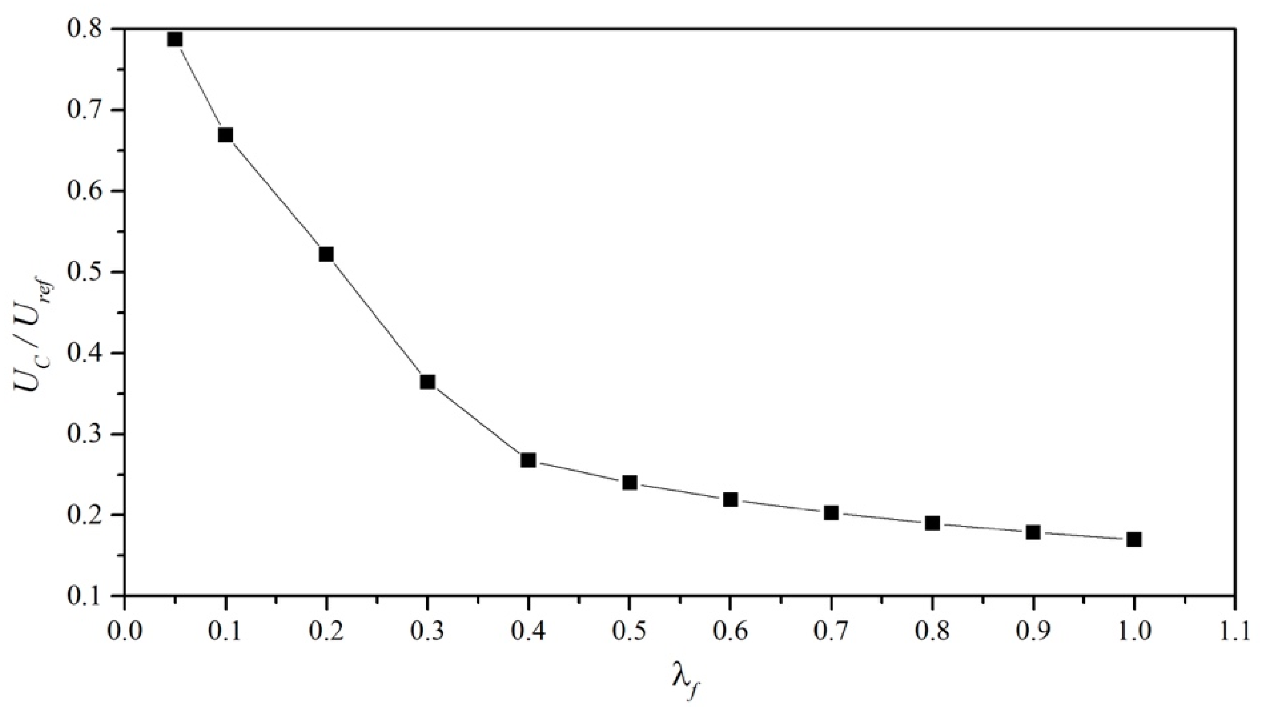
The relationship between roughness height $z_0$, zero displacement $z_d$, frontal area ratio ${\lambda }_f$ and plan area ratio ${\lambda }_p$ from Grimmond and Oke [45] was directly used in the mentioned study, and was also adopted in this study. Combining these parameters with Equations (10)–(13), the relationship between frontal area ratio ${\lambda }_f$ and $U_c$ is shown in Figure 7. When ${\lambda }_f$ increases, the velocity in the urban canopy decreases.

The effective velocity $v_0$ can be rewritten to a function of $U_{ref}$. The rural wind follows the log law (Equation (8)), and $U_{ref}$ is the wind at 2H. Effective velocity can be calculated by Equation (14).

$$v_0=\frac{U_{ref}}{H}{\displaystyle \underset{0}{\overset{H}{\int }}\ln \left(\frac{z-z_{ref}}{z_0}\right)}dz$$

(14)

The length of the city L is proportional to the building height H. $L/H=l$. Equation (8) becomes

$$\frac{q}{U_{ref}{H}^2}=\frac{\mathrm{L}\sqrt{1-{\lambda }_p}}{\mathrm{H}}\left(\left(\ln \frac{H}{z_0}-1\right)/\ln \left(\frac{2H}{z_0}\right)\right)+\left[\left(\mathrm{L}-\frac{x_0}{H}\right)L\right]\left(1-{\lambda }_p\right)\frac{U_E}{U_{ref}}$$

(15)

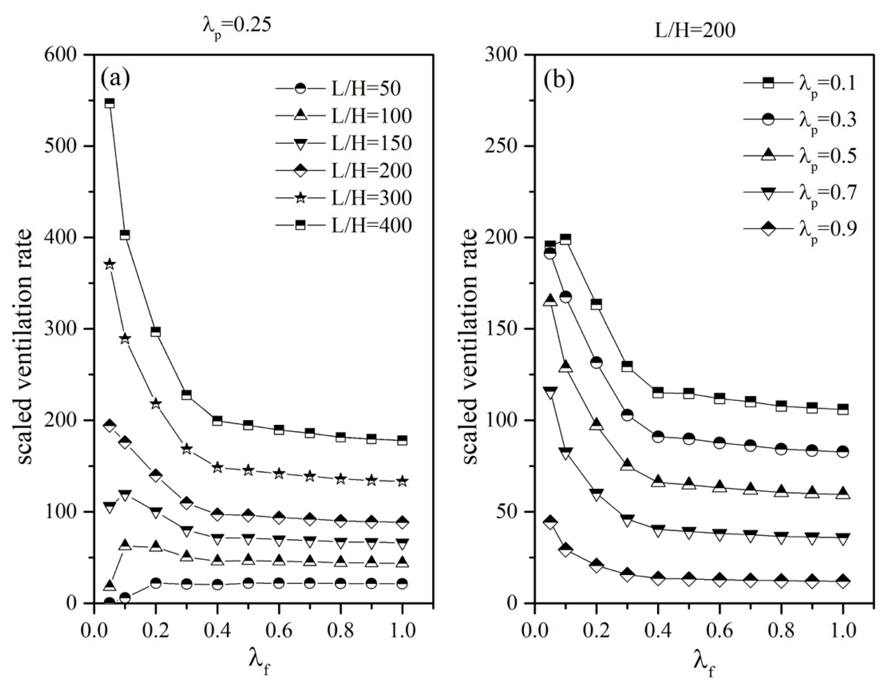
Figure 8a shows the total air change rate with different city length and ${\lambda }_f$. The density (${\lambda }_P$) is 0.25. In general, the ventilation rate is larger when the city is bigger. Because the area dominated by vertical velocity, which is the after-penetration area, is larger than the area in the small city. When the city is large enough (larger than 200 H), the ventilation rate decreases with ${\lambda }_f$. This is because the city has large ${\lambda }_f$ usually has large H/W ratio, which leads to small exchange velocity. However, for the small city, the ventilation rate increases first when ${\lambda }_f$ is smaller than 0.2. When ${\lambda }_f$ increases, the penetration depth ($x_0$) decreases, and term $\left[\left(L-x_0\right)L\right]$ increase, while the exchange velocity decreases. Therefore, a maximum ventilation rate appears when ${\lambda }_f$ is 0.2. A large city is usually larger than 200 H long. We used L/H = 200 as a constant to discuss the impact of ${\lambda }_P$. Figure 8b shows the ventilation rate with different ${\lambda }_p$ and ${\lambda }_f$ for a general city (L/H = 200). When ${\lambda }_p$ increases, the city becomes more compact, and the ventilation rate smaller.

3.3. Anthropogenic Heat

In the ideal city, the distribution of anthropogenic heat is assumed to be uniform. The anthropogenic heat includes several parts: metabolism, industry, buildings and transports.

(a)

The heat flux generated from metabolism, industry and buildings

In the study area (i.e., District Yau Tsim Mong), the population density is 40,000 persons per square kilometer [49], and the corresponding metabolic heat flux is on the order of 10 W m⁻² [50]. The heat flux generated from industry is ignored as there is almost no industry [51]. The heat flux generated from buildings is calculated by Equation (16) according to Sailor [50] and Yang et al. [41].

$$q_{anth}=\frac{A_r{q}_{anth,b}\left(H/H_{floor}\right)}{A_b}$$

(16)

where $q_{anth,b}$ is 50 W m⁻² and the $H_{floor}$ is the height of each floor, which is assumed to be 3 m.

(b)

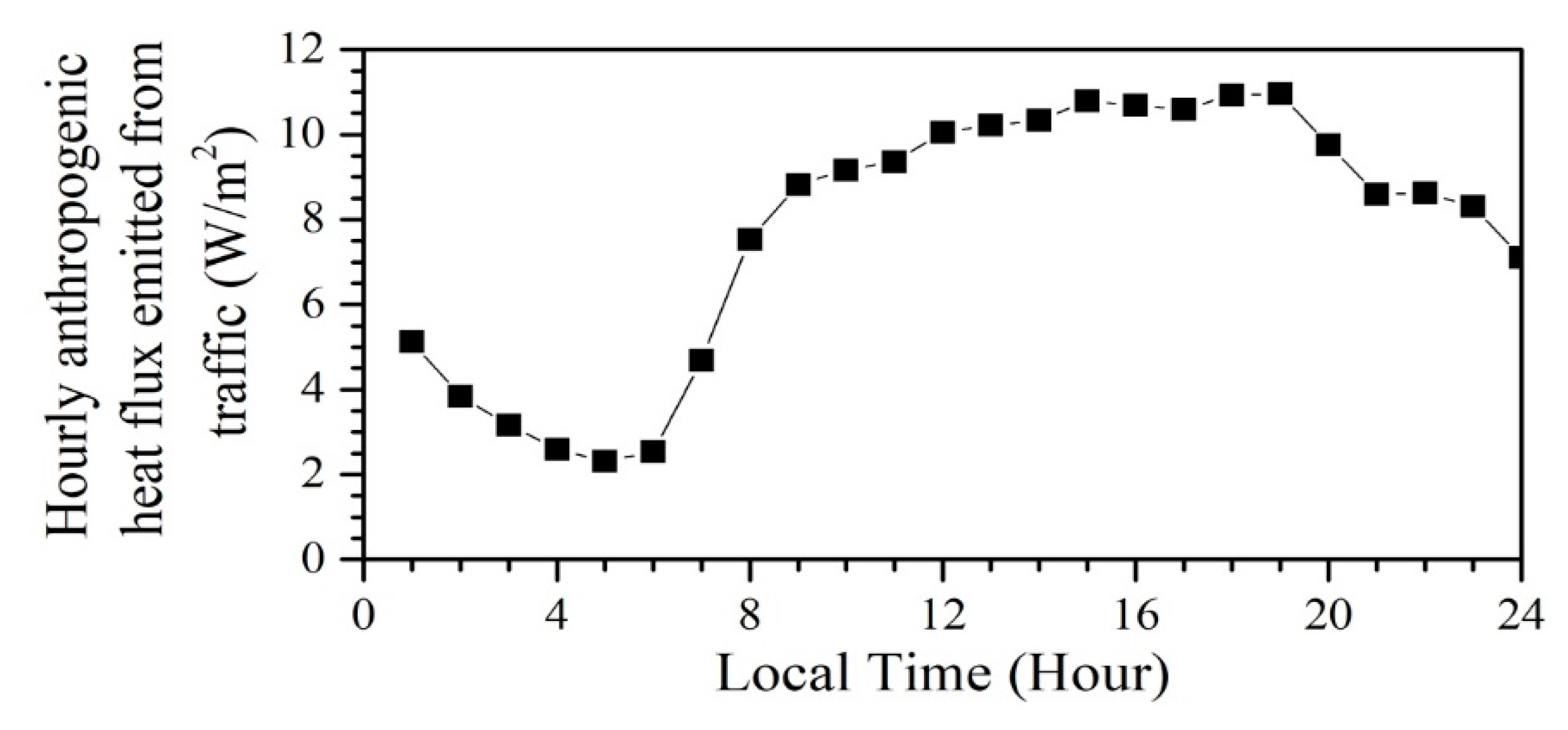
The heat flux generated from traffic

The hourly anthropogenic heat flux emitted from traffic $q_{tra}(hr)$ is calculated from Equation (17) [52,53].

$$q_{tra}(hr)=\left[{\displaystyle \sum _{ijk}\left(n_{vijk}(hr)\times q_{v\_ij}\times d_k\right)}/3600\right]/A_p$$

(17)

where $h$ is local time, $n_{vijk}(h)$ is the hourly total number of vehicles of class $i$ consuming fuel type $j$ and travelling on road segment $k$ at hour $h$, $q_{v\_ij}$ (J m⁻¹) is the energy used per vehicle of class $i$ consuming fuel type $j$, and $d_k$ is the vehicle distance travelled on road segment $k$ (m).

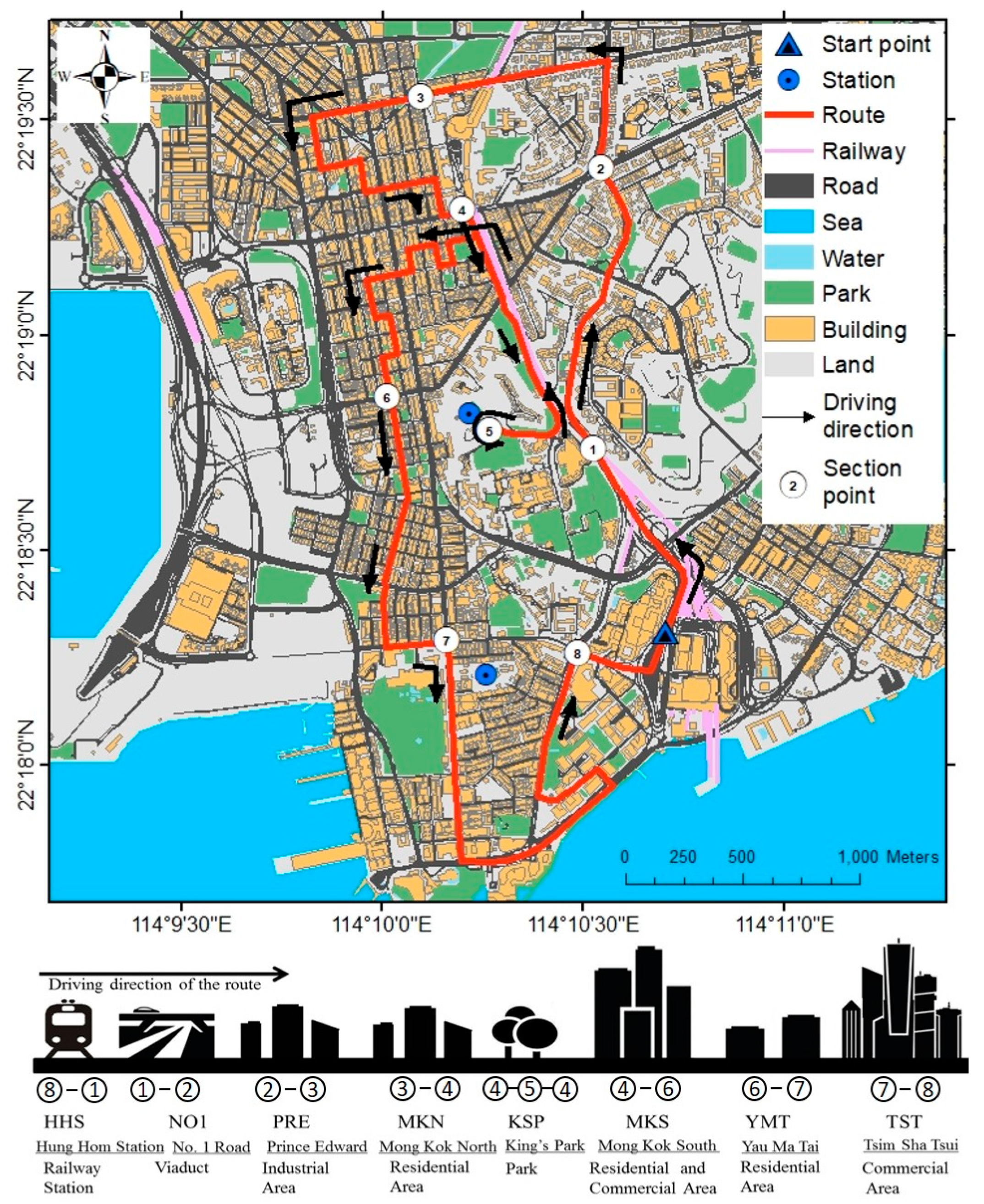
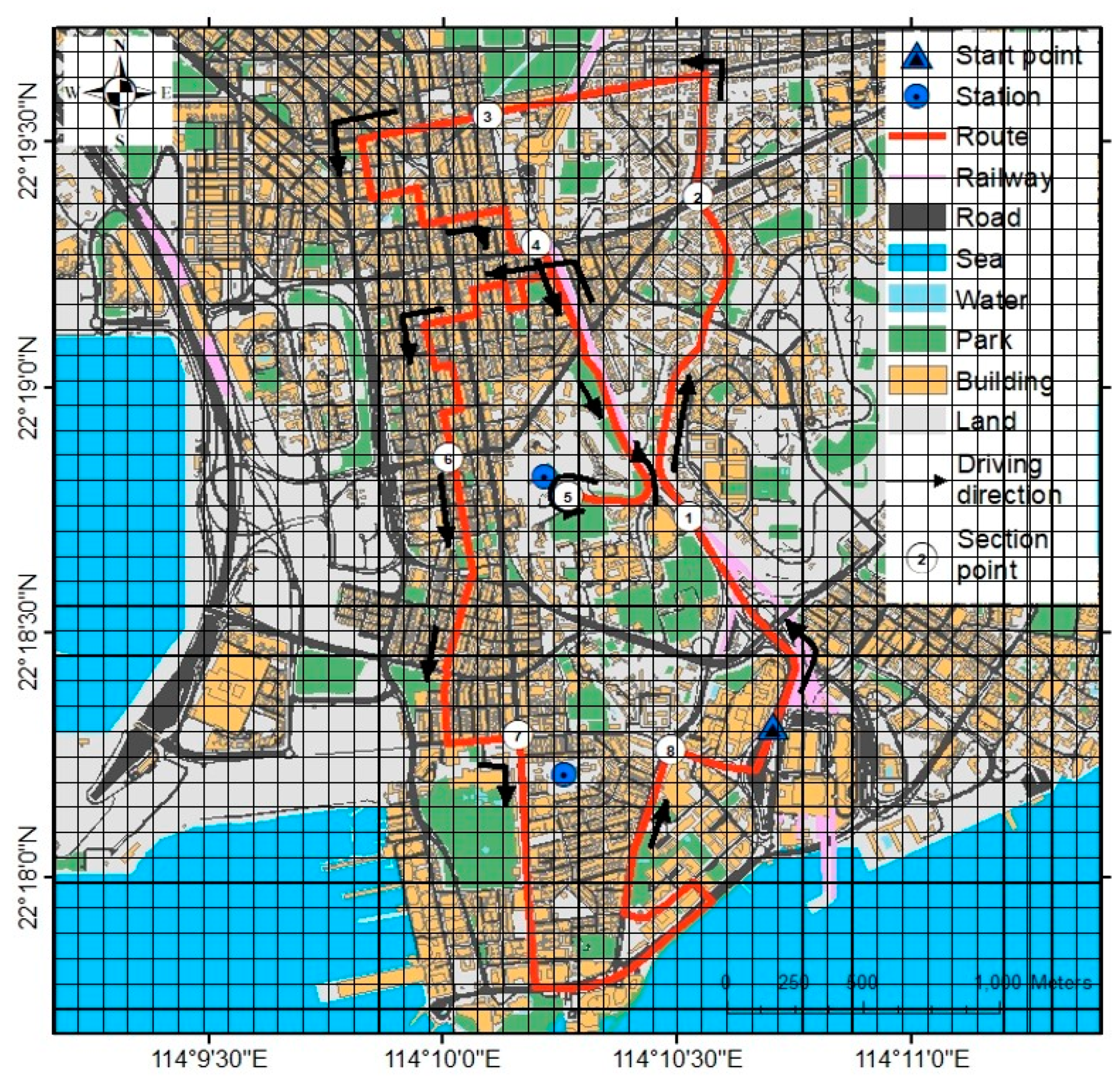
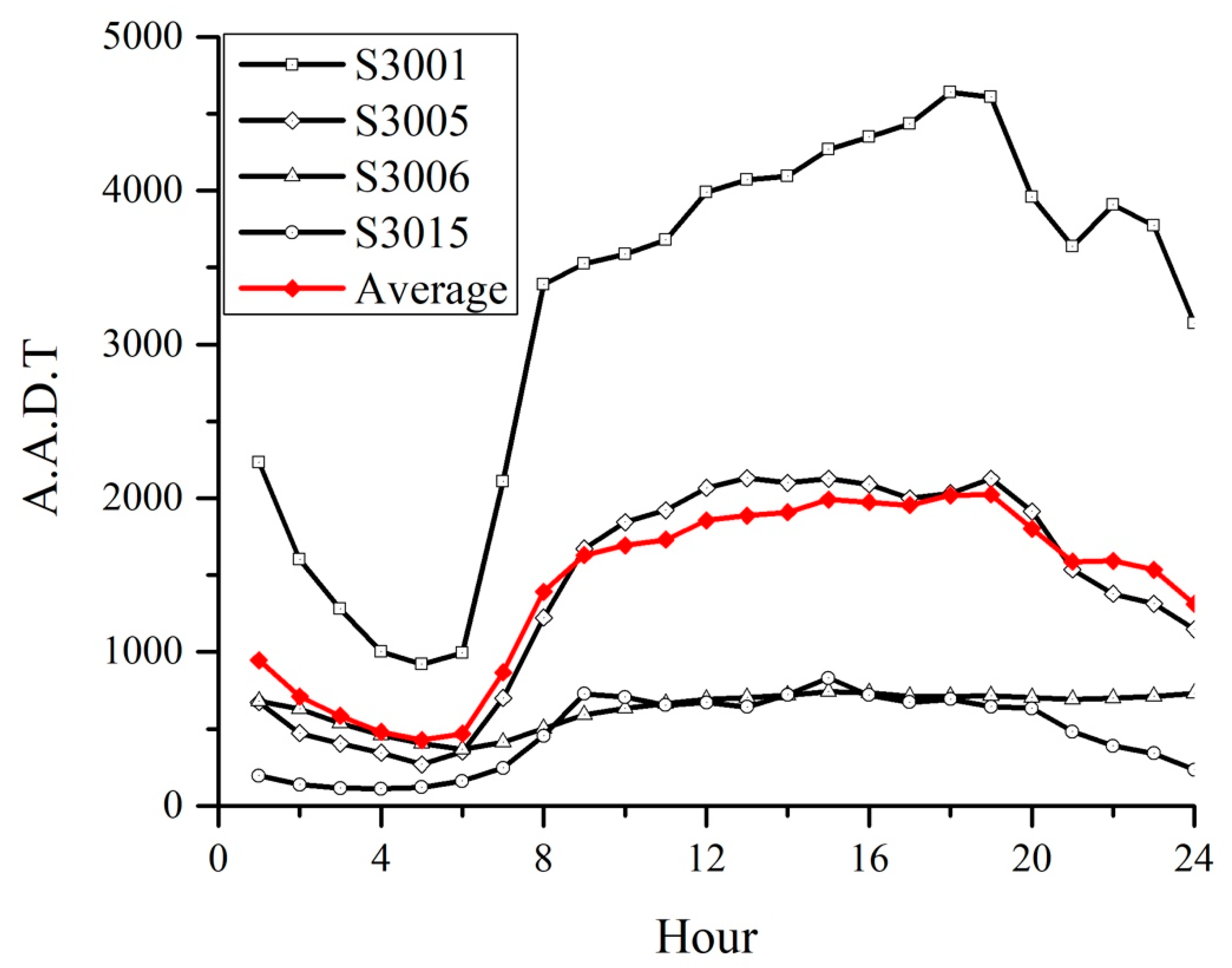
Assume the traffic flow in the ideal city is uniform. We averaged the Annual Average Daily Traffic (A.A.D.T) from four monitored station in the different part of the design route [54], and used it as the uniform traffic flow. The averaged A.A.D.T are shown in Appendix C.

Table 2. Energy consumption and its percentage of each vehicle class type ¹.

Vehicle Type	Goods Vehicle	Car	Bus	Taxi	Motorcycle
Percentage (%)	35.93%	23.80%	22.82%	16.91%	0.54%
Energy used per vehicle (J m−1)	9119.3	4210.8	16698.4	4001.8	1183.2

¹ Calculated from annual traffic census [54].

shows the percentage of each class among the vehicles and the energy used for each vehicle class in Hong Kong. The latter was similar to Singapore [53]. It was assumed all cars in Hong Kong use unleaded petrol. The total area and total road length of the road segment are evaluated from Google Earth. 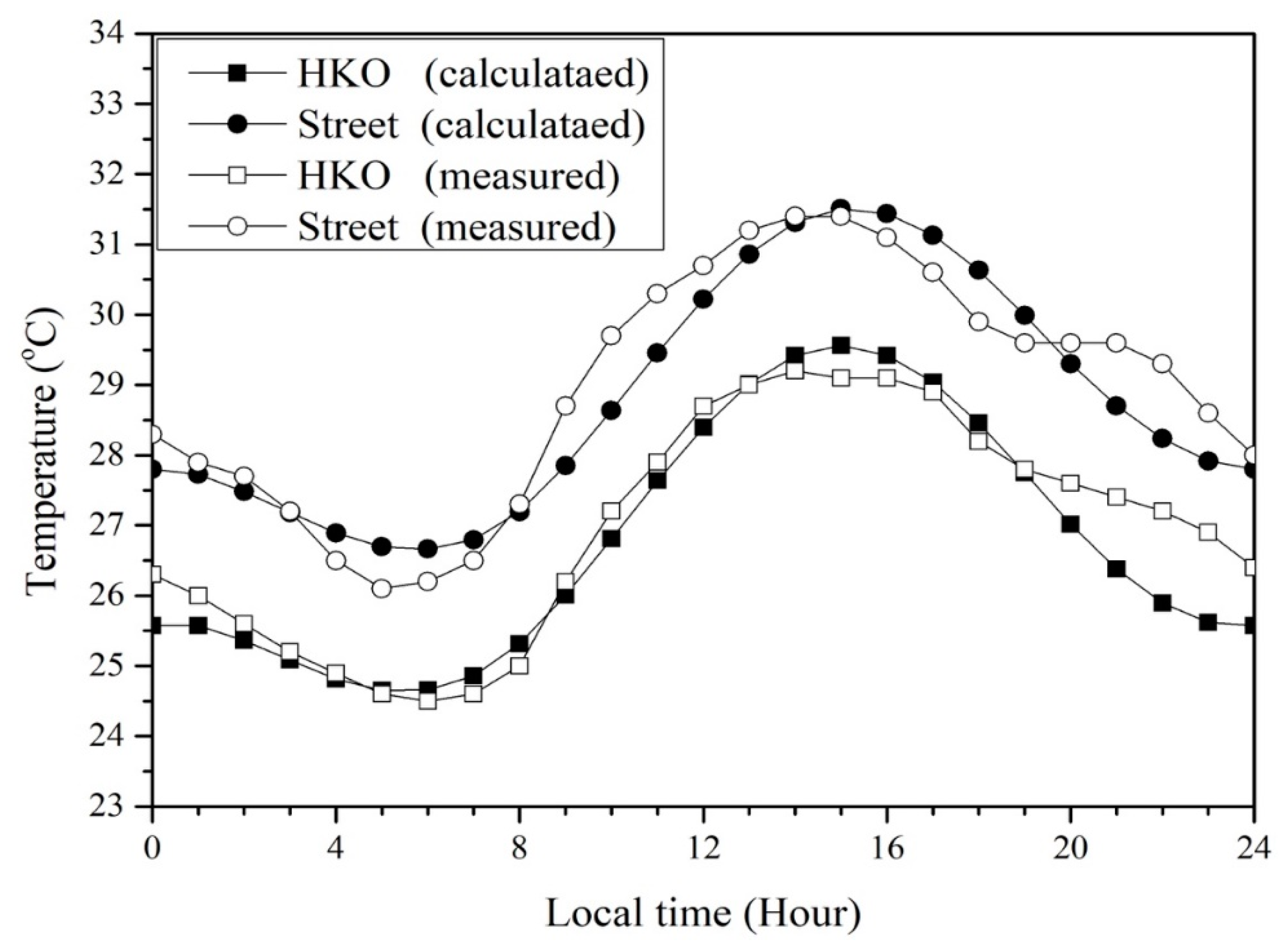Finally, the hourly anthropogenic heat flux released from transport in the experiment area was calculated, as shown in Figure 9.

4. Results

4.1. Data Mining Process

One of the key issues for this traverse experiment is to find the correct value to represent the temperature of the whole experiment area at the right time. The general method (Method 1) is to average all the measured points in each hour (from 00 to 59 min). Meanwhile, to avoid noise in the measurement, we can extract the main characteristics of the street temperature through the Fast Fourier transformation (FFT) method (Method 2). The first and the second harmonics of measured data were extracted, and the extracted diurnal cycle was considered as the average temperature of the area [55]. The point value measured from 00 to 59 min was used to represent that hour. Due to the small bias of the GPS coordinate during the experiment, we used the “cell” (as defined above) to represent the location, as discussed in Figure 4. Only the data of a whole day (0:00–23:59) were used for FFT analysis. The missing data were filled by three-point interpolation when there were only one or two continuous hours missing; the data were ignored when more than three hours were missing.

In the experiment, the measured data could only actually represent a small area. During the experimental period, the average diurnal temperature range (DTR), which is the difference between maximum and minimum air temperature [56] was larger than 15 °C. The temperature change rate (TCR), which is the range of temperature change per hour, can be calculated by dividing the DTR by 24. This shows how fast the temperature changes hourly, thus when the TCR is large, the temperature increases sharply. In this experiment, TCR can be above 1 °C per hour. Considering that one hour was required to complete one loop, the error between two locations could be more than 1 °C without considering the spatial difference. Thus, we also considered the interpolation method here. The average temperatures calculated by Method 1 were used for interpolation. The piecewise Hermit method was used to interpolate the temperature to each time point (e.g., 1:00, 2:00, etc.) (Method 3). Then temperatures at the same time point were averaged.

Figure 10 shows the hourly average street temperature profiles from three different methods. For most of the time, the average temperature and the trends calculated by Method 1 (directly average) and Method 3 (average after interpolation) are similar. However, the extreme values are filtered by Method 3. Meanwhile, Method 2 extracts the main character of the air temperature in the whole area. Actually, this is more representative for the experimental area. We also noticed that at night (around 20:00–24:00), the air temperature decreases very slowly. However, such character is not captured by Method 2. This is because such decrease at night is a short-term signal which cannot be captured by the first and second harmonies of measured data. Generally, Method 2 can reflect the main character of the air temperature values over the whole experimental area, and Method 3 is closest to the real temperature values, which are obtained by filtering the noise from the measured temperature values.

4.2. The Street Warming Phenomenon (Comparing Air Temperature in Streets and at HKO Monitoring Stations)

Figure 11 shows the hourly mean air temperature profiles and its standard deviations during three representative periods (P1–P3) in streets and three fixed stations. Among them, the HKO station located in an urban built-up area to represent the city temperature, KP station is in green area and Tsak Yue Wu (TYW) is a remote station to represent the rural air temperature [57]. The average street air temperatures were warmer than the rural temperatures, and were 1–3 °C higher than those recorded at fixed weather stations nearby. The temperature was underestimated when we use air temperature obtained from fixed weather station to represent the street air temperature. Similar phenomenon was found by Wong et al. [58]. Only using one point value or one value to represent the UHI for the whole city is not enough [27]. We termed the difference between the street temperature and rural temperature (T_street − T_rural) as the street urban heat island (sUHI) intensity. The sUHI intensity is rather small during the day, or sometimes even negative, particularly in the afternoon, which agrees with the urban cool island phenomenon [39]. Compared to the previous UHI in Hong Kong [4], sUHI is more realistic for practical purpose because it uses air temperature at street level instead of the air temperature at urban weather stations to present the urban temperature. The latter ones are mostly located in open green areas or natural earth [59]. The UHI in the street has been underestimated by about 2 °C on average. This significant difference is of interest to us as the streets are where people are, and where human activities take place.

4.3. Model Result

There are many differences between the environment in the street and that surrounding a fixed weather station. Temperatures in HKO station, often considered as city temperature, are compared with the temperature in the street. Figure 12 shows the environment around the temperature sensor in both HKO station (Figure 12a,b) and streets (Figure 12c,d). The underlying surface is very different in these two places. HKO station located in an open area covered by grass (Figure 12a), while in the street, the underlying surface is asphalt pavement (Figure 12c). The green area ratio ${\lambda }_{\mathrm{g}}$, which is the ratio of the area of the green zone ($A_g$) to total urban area ($A_p$), is also different. Meanwhile, from Figure 12b,d, it is easy to conclude that the plan area ratio ${\lambda }_p$ and frontal area ratio ${\lambda }_f$ of HKO station are smaller than that of streets, which lead to different ventilation rates.

The air temperature in the HKO station and in streets were simulated by improved zero-CAT model with the same anthropogenic heat (Section 3.3). Due to different ${\lambda }_p$ and ${\lambda }_f$, the ventilation rates are different. Assume the experiment area is 4.9 × 10⁷ m², the building height is 40 m, and the date is 16 September 2012. The exchange velocity and ventilation rates calculated by different morphology parameters are shown in

Table 3. The different parameters used for the temperature simulation in the station and streets.

	Green Area Ratio	$\mathbf{Frontal}\mathbf{Area}\mathbf{Ratio}\left({\mathit{\lambda }}_{\mathit{f}}\right)$	$\mathbf{Plan}\mathbf{Area}\mathbf{Ratio}\left({\mathit{\lambda }}_{\mathit{p}}\right)$	H/W	${\mathit{U}}_{\mathit{E}} (\mathbf{m}/\mathbf{s})$	$\mathit{q} ({\mathbf{m}}^3/\mathbf{s})$
Station	0.40	0.50	0.30	6	0.0947	4.1255 × 106
Street	0.16	1.80	0.54	6	0.0824	2.4910 × 106

. The ventilation rate in the streets is much smaller than in the HKO station. Other different morphology parameters used for simulation are also shown in Table 3. The green area ratio is the green area over the whole experiment domain. Therefore, although the vegetation areas in Figure 12b,d are totally different, the difference between vegetation area ratio in the stations scenario and streets scenario are smaller. Other settings such as thermal mass, soil temperature, etc. are the same.

Figure 13 shows the measured and simulated air temperature in HKO station and in streets. The simulated temperatures agree well with the measured ones except in the evening. The range of temperature, average temperature and the time when maximum temperature appears are similar between the simulated and measured temperatures. The average temperature in streets is 2 °C higher than at HKO station. This shows the ability of the improved zero-CAT model to predict temperatures in the street canyon.

4.4. Sensitivity Analysis for Urban Design

The urban morphology parameters, including H/W ratio, plan area ratio (${\lambda }_p$) and frontal area ratio (${\lambda }_f$), are important indicators for thermal comfort. To improve thermal comfort, the ambient air temperature and net radiation (including short wave radiation and long wave radiation) should be all considered, while the air temperature is an important factor and is the one we are focused here. For sensitivity studies, we used the same settings as the previous simulation in the street (Section 4.3) but change the green area ratio to 0. Figure 14 shows the daily air temperature profiles when plan area ratio (${\lambda }_p$) is different. When ${\lambda }_p$ increased from 0.1 to 0.9, which means the city became compact, the average air temperature increased almost by 1 °C. The DTR decreased from 6.4 °C to 2.8 °C and the maximum air temperature increased from 31.3 °C to 39.0 °C. The time when the maximum air temperature appears (Time-max) delayed more than 1 h, from before 15:00 to 16:00. The minimum temperature increased from 25.0 °C to 36.1 °C, and the time of minimum temperature appears delayed from 5:00 to 7:00.

When H/W ratio and plan area ratio (${\lambda }_p$) change at the same time with frontal area ratio (${\lambda }_f$), the analysis is more complicated. We use four parameters, including the average temperature, DTR, the maximum air temperature and Time-max (defined as time when the maximum temperature appears of the daily temperature) to qualify the contribution of the urban morphology parameters, as shown in Figure 15. Due to the pronounced hysteresis effects for the full diurnal cycles of air and surface temperature at local scale, the time when the maximum temperature appears during the days is not at noon [31]. The anthropogenic heat in all the simulations are the same. No matter what H/W ratio and plan area ratio (${\lambda }_p$) are adopted, the lowest mean air temperature and maximum temperature appear when frontal area ratio (${\lambda }_f$) is 0.2. The diurnal temperature range is the largest. When frontal area ratio (${\lambda }_f$) is larger than 0.4, the ventilation rate decreases very slowly, and the temperature increases slightly. Therefore, despite plan area ratio (${\lambda }_p$) and H/W ratio, for urban designers, keeping frontal area ratio (${\lambda }_f$) in the dominate wind direction around 0.2 is the best for low air temperature in streets. H/W ratio has large impact on the maximum temperature, but slightly changes the average air temperature. With the increase of the H/W ratio, the average air temperature decreases slightly, and the maximum air temperature decreases too. High H/W ratio also leads to late Time-max and small DTR, which indicates increasing the H/W ratio could also keep the street temperature cool. On the contrast, the average air temperature increases significantly when plan area ratio (${\lambda }_p$) increases. As discussed before, high plan area ratio (${\lambda }_p$) leads to high average temperature and maximum air temperature, small DTR and late Time-max.

Finally, these parameters together also influence the anthropogenic heat from buildings, and the effect of all of them is rather complicated for analyses. We categorized five scenarios that are commonly found in existing cities. The parameters of these five scenarios are shown in

Table 4. The urban morphology of the five scenarios.

Scenario	1 (LS)	2 (HS-high H/W)	3 (HS-low H/W)	4 (LC)	5 (HC)
${\lambda }_p$	0.25	0.25	0.25	0.64	0.64
H/W ratio	1	6	4.8	1	6
${\lambda }_f$	0.25	1.5	1.5	0.16	0.96
Average building height	10	60	24	4	24

. Assuming the total control volume and plan area is the same among the five scenarios, the average building height changes due to changes in the urban morphology parameters. Scenario 1 is the low-rise low-density city, which is low and sparse, referred to as LS; Scenarios 2 and 3 are high-rise low-density city with different height and H/W ratio, which is high and sparse, referred to as HS; Scenario 4 is low-rise high-density city, which is low and compact, referred to as LC; and Scenario 5 is high-rise high-density city, which is high and compact, referred to as HC. Meanwhile, since the height of the building is not the same, the anthropogenic heat generated from buildings are different according to Equation (16).

The simulated air temperatures are shown in Figure 16. The highest temperature occurred in the low and compact city. In the HS scenario, diurnal temperature range was the lowest. Although the H/W ratio and building height in Scenario 2 (HS-high H/W) were larger than those in Scenario 3 (HS-low H/W), the air temperature value in Scenarios 1 and 3 did not differ much. Further discussion is given in Section 5.

5. Discussion

5.1. The Underestimation of the Early Night in the Model

The underestimation of the model can be attribute to high energy consumption on summer evenings in Hong Kong. Tso and Yau [60] studied domestic energy usage patterns in Hong Kong, and found that energy consumption increases sharply from 18:00 to 19:00, and the peak hour is around 22:00, after which, energy consumption decreases slowly. This is accounted for by the use of air-conditioners in summer time to cool room temperatures when returning home and sleeping. Such increase in energy consumption leads to rising ambient air temperatures in the evening [61]. The underestimation can be improved by calculating the anthropogenic heat from buildings based on daily energy consumption. It is worth mentioning that the aim of this method is to predict the average air temperature among several or many blocks, such as in the city center, especially for cases that are impossible to simulate with the CFD model.

5.2. The Performance of Different Urban Form

We evaluated five different scenarios in Section 4.4 which could present five different urban forms. The results show that the trend of temperature variation in daytime and nighttime is very different. At night, the air temperature in the street is lower when the average building height is low, or referred to as the low city. This can be attributed to the small effective thermal storage in the low city, which releases less heat compared to the high city at night [62]. The air temperature is also lower in the sparse city than in the compact city, due to decreasing urban albedo and increasing shading area [39,63]. Therefore, the air temperature is the highest in the high and compact city at night.

During the daytime, the situation is different. From the results, the street air temperature is lower in high and sparse city. However, previous studies [39,62] found that high and compact cities usually have lower air temperature during the daytime compared to rural areas. This may look confusing but actually the observations do not conflict. When city density is fixed, the temperature is lower among the higher city, as shown in Scenarios 2 and 3 in Figure 16. When the average height of buildings and the control volume of the study area are fixed, the total number of residences for the compact city is much higher, which lead to larger heat flux generated from buildings, and larger effective thermal storage. Therefore, street air temperature in the street in the compact city is higher than in the sparse city, as shown in Scenarios 3 and 5 (Figure 16). It is worth mentioning that some assumptions of the model are based on the situation in Hong Kong, in which we aim for cool temperature in the daytime. For the other area in the world, the aim of the city designer may be warm air temperature during day or night, thus they may use different parameters from the study.

5.3. Importance and Extended Implications of the Model

The underestimation of the street air temperature was also reported by Wong et al. [58]. The improved numerical model could correct such underestimation. This is very important for further analysis of the urban environment. In a city, streets are important common areas for people’s daily life. Based on our model with suitable parameters, we can rapidly obtain accurate street air temperature in the city. Greater accuracy of street air temperature and magnitude of the urban heat island could help decision-makers in mitigating the urban heat island and in preparing for future heat waves and other extreme events. Moreover, it could help city designers to know whether their designs could contribute to better thermal comfort for the city. Greater accuracy of air temperature is also useful for the study of thermal comfort, urban environment, and pollutant dispersion.

5.4. Limitation and Future Work

One of the limitation is that the experiment was taken during sunny days, and both the experiment and the model did not consider the effect of the clouds, which is important in determining air temperature [26]. Besides, the validation experiments were only conducted in Hong Kong and performance of the model in other regions still needs validation. One more limitation is the lack of comparison with remote sensing technique. We leave the exploration of these limitations to the future.

6. Conclusions

A 24-h vehicle traverse study was conducted over the Kowloon Peninsula of Hong Kong in summer, with each measurement period consisting of 2–3 full days. The data covered 158 loops in 198 h along the route on sunny days. The data were averaged by three methods (direct average, FFT filter, and piecewise cubic Hermite interpolation). In the experiment, the average diurnal temperature range was more than 15 °C along the route, which gives rise to an average temperature which can change by more than 1 °C per hour, which was the time when one loop was completed. The FFT filter method produces the main character of the air temperature over the whole experimental area, and the interpolation method gives closest to the real temperature values, by filtering the noise from the measured temperature values.

The averaged street air temperatures were found to be 1–3 °C higher than those recorded at nearby fixed weather stations, due to the difference in the underlying surfaces and surrounding areas, ventilation and anthropogenic heat in the streets and weather stations. The air temperature and the corresponding urban heat island were underestimated. The results have substantial implications, as most previous UHI intensities were estimated from measurements at fixed weather stations, which are usually in parks or open areas. The UHI intensity in the street has been underestimated by an average of 2 °C. This significant difference is important for studies of outdoor thermal comfort, urban environment, and pollutant dispersion. We also improved a canopy layer temperature model (zero-CAT) for predicting the urban air temperatures in the street, and, at stations, by using different urban morphology parameters. The model was validated by the air temperature transects, and shows good ability to predict the air temperature in streets, and for correcting underestimated temperatures. The contributions of urban morphology parameters were also analyzed by sensitivity studies. A high frontal area ratio (${\lambda }_p$) leads to high average temperature and maximum air temperature, while high H/W ratio usually leads to low maximum air temperature. Both parameters are accompanied by small diurnal temperature range and delayed time of maximum air temperature. Additionally, the study found that the frontal area ratio (${\lambda }_f$) is a key value for controlling air temperature in the street.

References

1. Ali-Toudert, F.; Mayer, H. Thermal comfort in an east–west oriented street canyon in Freiburg (Germany) under hot summer conditions. Theor. Appl. Climatol. 2007, 87, 223–237. [Google Scholar] [CrossRef]
2. Hwang, R.L.; Lin, T.P.; Matzarakis, A. Seasonal effects of urban street shading on long-term outdoor thermal comfort. Build. Environ. 2011, 46, 863–870. [Google Scholar] [CrossRef]
3. Coutts, A.M.; White, E.C.; Tapper, N.J.; Beringer, J.; Livesley, S.J. Temperature and human thermal comfort effects of street trees across three contrasting street canyon environments. Theor. Appl. Climatol. 2016, 124, 55–68. [Google Scholar] [CrossRef]
4. Wing-Lui, G.; Tsz-Cheung, L.; Chan, K.Y. Past and Future Changes in the Climate of Hong Kong. J. Meteorol. Res. 2010, 24, 163–175. [Google Scholar]
5. Taleghani, M.; Kleerekoper, L.; Tenpierik, M.; van den Dobbelsteen, A. Outdoor thermal comfort within five different urban forms in The Netherlands. Build. Environ. 2015, 83, 65–78. [Google Scholar] [CrossRef]
6. Oke, T.R. Siting and exposure of meteorological instruments at urban sites. In Proceedings of the 27th NATO/CCMS International Technical Meeting on Air Pollution Modelling and its Application, Banff, Canada, 25–29 October 2004; Springer: Boston, MA, USA, 2007; pp. 615–631. [Google Scholar]
7. Conrads, L.A.; van der Hage, J.C.H. A new method of air-temperature measurement in urban climatological studies. Atmos. Environ. 1971, 5, 629–635. [Google Scholar] [CrossRef] [Green Version]
8. Tso, C.P. A survey of urban heat island studies in two tropical cities. Atmos. Environ. 1996, 30, 507–519. [Google Scholar] [CrossRef]
9. Deosthali, V. Impact of rapid urban growth on heat and moisture islands in Pune City, India. Atmos. Environ. 2000, 34, 2745–2754. [Google Scholar] [CrossRef]
10. Zhao, Q.; Sailor, D.J.; Wentz, E.A. Impact of tree locations and arrangements on outdoor microclimates and human thermal comfort in an urban residential environment. Urban For. Urban Green. 2018, 32, 81–91. [Google Scholar] [CrossRef]
11. Wong, N.H.; Yu, C. Study of green areas and urban heat island in a tropical city. Habitat Int. 2005, 29, 547–558. [Google Scholar] [CrossRef]
12. Saitoh, T.S.; Shimada, T.; Hoshi, H. Modeling and simulation of the Tokyo urban heat island. Atmos. Environ. 1996, 30, 3431–3442. [Google Scholar] [CrossRef]
13. Nakamura, Y.; Oke, T. Wind, temperature and stability conditions in an east-west oriented urban canyon. Atmos. Environ. (1967) 1988, 22, 2691–2700. [Google Scholar] [CrossRef]
14. Oke, T.R. Street design and urban canopy layer climate. Energy Build. 1988, 11, 103–113. [Google Scholar] [CrossRef]
15. Arnfield, A.J. Two decades of urban climate research: A review of turbulence, exchanges of energy and water, and the urban heat island. Int. J. Climatol. 2003, 23, 1–26. [Google Scholar] [CrossRef]
16. Sini, J.F.; Anquetin, S.; Mestayer, P.G. Pollutant dispersion and thermal effects in urban street canyons. Atmos. Environ. 1996, 30, 2659–2677. [Google Scholar] [CrossRef]
17. Shashua-Bar, L.; Hoffman, M.E. Vegetation as a climatic component in the design of an urban street: An empirical model for predicting the cooling effect of urban green areas with trees. Energy Build. 2000, 31, 221–235. [Google Scholar] [CrossRef]
18. Uehara, K.; Murakami, S.; Oikawa, S.; Wakamatsu, S. Wind tunnel experiments on how thermal stratification affects flow in and above urban street canyons. Atmos. Environ. 2000, 34, 1553–1562. [Google Scholar] [CrossRef]
19. Vardoulakis, S.; Fisher, B.E.; Pericleous, K.; Gonzalez-Flesca, N. Modelling air quality in street canyons: A review. Atmos. Environ. 2003, 37, 155–182. [Google Scholar] [CrossRef]
20. Eliasson, I.; Offerle, B.; Grimmond, C.S.B.; Lindqvist, S. Wind fields and turbulence statistics in an urban street canyon. Atmos. Environ. 2006, 40, 1–16. [Google Scholar] [CrossRef]
21. Chow, W.T.L.; Roth, M. Temporal dynamics of the urban heat island of Singapore. Int. J. Climatol. 2006, 26, 2243–2260. [Google Scholar] [CrossRef] [Green Version]
22. Santamouris, M.; Papanikolaou, N.; Koronakis, I.; Livada, I.; Asimakopoulos, D. Thermal and air flow characteristics in a deep pedestrian canyon under hot weather conditions. Atmos. Environ. 1999, 33, 4503–4521. [Google Scholar] [CrossRef]
23. Georgakis, C.; Santamouris, M. Experimental investigation of air flow and temperature distribution in deep urban canyons for natural ventilation purposes. Energy Build. 2006, 38, 367–376. [Google Scholar] [CrossRef]
24. Erell, E.; Williamson, T. Simulating air temperature in an urban street canyon in all weather conditions using measured data at a reference meteorological station. Int. J. Climatol. 2006, 26, 1671–1694. [Google Scholar] [CrossRef] [Green Version]
25. Zhao, Q.; Wentz, E.A. A MODIS/ASTER airborne simulator (MASTER) imagery for urban heat Island research. Data 2016, 1, 7. [Google Scholar] [CrossRef]
26. Hu, L.; Monaghan, A.J.; Brunsell, N.A. Investigation of urban air temperature and humidity patterns during extreme heat conditions using satellite-derived data. J. Appl. Meteorol. Climatol. 2015, 54, 2245–2259. [Google Scholar] [CrossRef]
27. Schwarz, N.; Schlink, U.; Franck, U.; Großmann, K. Relationship of land surface and air temperatures and its implications for quantifying urban heat island indicators—An application for the city of Leipzig (Germany). Ecol. Indic. 2012, 18, 693–704. [Google Scholar] [CrossRef]
28. Myint, S.W.; Brazel, A.; Okin, G.; Buyantuyev, A. Combined effects of impervious surface and vegetation cover on air temperature variations in a rapidly expanding desert city. GISci. Remote Sens. 2010, 47, 301–320. [Google Scholar] [CrossRef]
29. Fung, W.Y.; Lam, K.S.; Nichol, J.; Wong, M.S. Derivation of nighttime urban air temperatures using a satellite thermal image. J. Appl. Meteorol. Climatol. 2009, 48, 863–872. [Google Scholar] [CrossRef]
30. Nichol, J.E.; Fung, W.Y.; Lam, K.S.; Wong, M.S. Urban heat island diagnosis using ASTER satellite images and ‘in situ’air temperature. Atmos. Res. 2009, 94, 276–284. [Google Scholar] [CrossRef]
31. Song, J.; Wang, Z.H.; Myint, S.W.; Wang, C. The hysteresis effect on surface-air temperature relationship and its implications to urban planning: An examination in Phoenix, Arizona, USA. Landsc. Urban Plan. 2017, 167, 198–211. [Google Scholar] [CrossRef]
32. Li, X.X.; Liu, C.H.; Leung, D.Y.C.; Lam, K.M. Recent progress in CFD modelling of wind field and pollutant transport in street canyons. Atmos. Environ. 2006, 40, 5640–5658. [Google Scholar] [CrossRef]
33. Li, X.X.; Liu, C.H.; Leung, D.Y.C. Numerical investigation of pollutant transport characteristics inside deep urban street canyons. Atmos. Environ. 2009, 43, 2410–2418. [Google Scholar] [CrossRef]
34. Giridharan, R.; Ganesan, S.; Lau, S.S.Y. Daytime urban heat island effect in high-rise and high-density residential developments in Hong Kong. Energy Build. 2004, 36, 525–534. [Google Scholar] [CrossRef]
35. Giridharan, R.; Lau, S.S.Y.; Ganesan, S.; Givoni, B. Urban design factors influencing heat island intensity in high-rise high-density environments of Hong Kong. Build. Environ. 2007, 42, 3669–3684. [Google Scholar] [CrossRef]
36. Giridharan, R.; Lau, S.S.Y.; Ganesan, S. Nocturnal heat island effect in urban residential developments of Hong Kong. Energy Build. 2005, 37, 964–971. [Google Scholar] [CrossRef]
37. Silva, H.R.; Bhardwaj, R.; Phelan, P.E.; Golden, J.S.; Grossman-Clarke, S. Development of a zero-dimensional mesoscale thermal model for urban climate. J. Appl. Meteorol. Climatol. 2009, 48, 657–668. [Google Scholar] [CrossRef]
38. Yang, L.; Li, Y. City ventilation of Hong Kong at no-wind conditions. Atmos. Environ. 2009, 43, 3111–3121. [Google Scholar] [CrossRef] [Green Version]
39. Yang, X.; Li, Y.; Luo, Z.; Chan, P.W. The urban cool island phenomenon in a high-rise high-density city and its mechanisms. Int. J. Climatol. 2016, 37, 890–904. [Google Scholar] [CrossRef]
40. Hang, J.; Li, Y.; Sandberg, M.; Buccolieri, R.; Di Sabatino, S. The influence of building height variability on pollutant dispersion and pedestrian ventilation in idealized high-rise urban areas. Build. Environ. 2012, 56, 346–360. [Google Scholar] [CrossRef]
41. Yang, X. Temporal Variation of Urban Surface and Air Temperature. Ph.D. Thesis, The University of Hong Kong, Pokfulam, Hong Kong, 2013. [Google Scholar]
42. Wong, M.S.; Nichol, J.E.; Ng, E. A study of the “wall effect” caused by proliferation of high-rise buildings using GIS techniques. Landsc. Urban Plan. 2011, 102, 245–253. [Google Scholar] [CrossRef]
43. Oke, T.R. The distinction between canopy and boundary-layer urban heat islands. Atmosphere 1976, 14, 268–277. [Google Scholar] [CrossRef]
44. Lyons, T.J.; Cutten, D.R. Atmospheric pollutant and temperature traverses in urban area. Atmos. Environ. 1975, 9, 731–737. [Google Scholar] [CrossRef]
45. Grimmond, C.S.B.; Oke, T.R. Aerodynamic properties of urban areas derived from analysis of surface form. J. Appl. Meteorol. 1999, 38, 1262–1292. [Google Scholar] [CrossRef]
46. Belcher, S.; Jerram, N.; Hunt, J. Adjustment of a turbulent boundary layer to a canopy of roughness elements. J. Fluid Mech. 2003, 488, 369–398. [Google Scholar] [CrossRef]
47. Bentham, T.; Britter, R. Spatially averaged flow within obstacle arrays. Atmos. Environ. 2003, 37, 2037–2043. [Google Scholar] [CrossRef]
48. Yuan, C.; Norford, L.; Ng, E. A Semi-Empirical Model for the Effect of Trees on the Urban Wind Environment. Landsc. Urban Plan. 2017, 168, 84–93. [Google Scholar] [CrossRef]
49. Results of the 2011 Population Census of Hong Kong. 2011. Available online: https://www.census2011.gov.hk/en/index.html (accessed on 11 October 2018).
50. Sailor, D.J. A review of methods for estimating anthropogenic heat and moisture emissions in the urban environment. Int. J. Climatol. 2011, 31, 189–199. [Google Scholar] [CrossRef] [Green Version]
51. Tang, W.S.; Lee, J.W.Y.; Ng, M.K. Public engagement as a tool of hegemony: The case of designing the new central harbourfront in Hong Kong. Crit. Sociol. 2012, 38, 89–106. [Google Scholar] [CrossRef]
52. Grimmond, C.S.B. The suburban energy balance: Methodological considerations and results for a mid-latitude west coast city under winter and spring conditions. Int. J. Climatol. 2010, 12, 481–497. [Google Scholar] [CrossRef]
53. Quah, A.K.; Roth, M. Diurnal and weekly variation of anthropogenic heat emissions in a tropical city, Singapore. Atmos. Environ. 2012, 46, 92–103. [Google Scholar] [CrossRef]
54. Annual Traffic Census 2012. 2012. Available online: https://www.td.gov.hk/filemanager/en/content_4635/annual%20traffic%20census%202012.pdf (accessed on 11 October 2018).
55. Wang, K.; Li, Y.; Wang, Y.; Yang, X. On the asymmetry of the urban daily air temperature cycle. J. Geophys. Res.-Atmos. 2017, 122, 5625–5635. [Google Scholar] [CrossRef]
56. Qu, M.; Wan, J.; Hao, X. Analysis of diurnal air temperature range change in the continental United States. Weather Clim. Extrem. 2014, 4, 86–95. [Google Scholar] [CrossRef]
57. Siu, L.W.; Hart, M.A. Quantifying urban heat island intensity in Hong Kong SAR, China. Environ. Monit. Assess. 2013, 185, 4383–4398. [Google Scholar] [CrossRef] [PubMed]
58. Wong, P.P.Y.; Lai, P.C.; Low, C.T.; Chen, S.; Hart, M. The impact of environmental and human factors on urban heat and microclimate variability. Build. Environ. 2016, 95, 199–208. [Google Scholar] [CrossRef]
59. Jarraud, M. Guide to Meteorological Instruments and Methods of Observation (WMO-No. 8); World Meteorological Organisation: Geneva, Switzerland, 2008; ISBN 978-92-63-10008. [Google Scholar]
60. Tso, G.K.; Yau, K.K. A study of domestic energy usage patterns in Hong Kong. Energy 2003, 28, 1671–1682. [Google Scholar] [CrossRef]
61. Fung, W.; Lam, K.S.; Hung, W.T.; Pang, S.W.; Lee, Y.L. Impact of urban temperature on energy consumption of Hong Kong. Energy 2006, 31, 2623–2637. [Google Scholar] [CrossRef]
62. Wang, K.; Li, Y.; Li, Y.; Lin, B. Stone forest as a small-scale field model for the study of urban climate. Int. J. Climat. 2018, 38, 3723–3731. [Google Scholar] [CrossRef]
63. Emmanuel, R.; Rosenlund, H.; Johansson, E. Urban shading—A design option for the tropics? A study in Colombo, Sri Lanka. Int. J. Climatol. 2007, 27, 1995–2004. [Google Scholar] [CrossRef]
Figure 1. The Kowloon Peninsula of Hong Kong, the bird’s eye view and street view of Mong Kok and associated weather stations (Hong Kong Observatory and King’s Park stations). Bird’s eye view pictures are from google map.
Atmosphere 09 00402 g001
Figure 2. (Top) The designed traverse route in the Kowloon Peninsula. (Bottom) Sketch of the features along the two designed routes.
Atmosphere 09 00402 g002
Figure 3. The experiment vehicle with installed sensors.
Atmosphere 09 00402 g003
Figure 4. The illustration of the cell among the route.
Atmosphere 09 00402 g004
Figure 5. A sketch of the simplified ideal city.
Atmosphere 09 00402 g005
Figure 6. A sketch of the penetration area and after the penetration area.
Atmosphere 09 00402 g006
Figure 7. The relationship between frontal area ratio ( λ f ) and velocity in the canopy layer ( U C ).
Atmosphere 09 00402 g007
Figure 8. The total air change rate with different city length, plan area ratio ( λ p ) and frontal area ratio ( λ f ): (a) λ p = 0.25 ; and (b) L / H = 200 .
Atmosphere 09 00402 g008
Figure 9. Hourly anthropogenic heat flux released from transports.
Atmosphere 09 00402 g009
Figure 10. Hourly average air temperature in the street calculated from three different averaging methods in different periods.
Atmosphere 09 00402 g010
Figure 11. The hourly average temperature in the street and three fix stations.
Atmosphere 09 00402 g011
Figure 12. (a) A picture of the surrounding environment, taken by the author; (b) an aerial photograph of the location around the HKO station from Google map; (c) a picture of the surrounding environment, taken by the author; and (d) an aerial photograph of the location in the street from Google map.
Atmosphere 09 00402 g012
Figure 13. The measured and simulated air temperature in the HKO station and in the street.
Atmosphere 09 00402 g013
Figure 14. The air temperature at 16 September 2012 when λ p (plan area ratio) is different.
Atmosphere 09 00402 g014
Figure 15. (a) The average air temperature; (b) the diurnal temperature range; (c) the maximum air temperature; and (d) the time when the maximum temperature appears of the diurnal temperature with different H/W ratio, plan area ratio ( λ p ) and frontal area ratio ( λ f ).
Atmosphere 09 00402 g015
Figure 16. Daily air temperature of the different scenarios.
Atmosphere 09 00402 g016