Characteristics of Gravity Waves over an Antarctic Ice Sheet during an Austral Summer

Abstract

While occurrences of wavelike motion in the stable boundary layer due to the presence of a significant restoring buoyancy force are rarely disputed, their modalities and interaction with turbulence remain a subject of active research. In this work, the characteristics of gravity waves and their impact on flow statistics, including turbulent fluxes, are presented using data collected above an Antarctic Ice sheet during an Austral Summer. Antarctica is an ideal location for exploring the characteristics of gravity waves because of persistent conditions of strong atmospheric stability in the lower troposphere. Periods dominated by wavelike motion have been identified by analysing time series measured by fast response instrumentation. The nature and characteristic of the dominant wavy motions are investigated using Fourier cross-spectral indicators. Moreover, a multi-resolution decomposition has been applied to separate gravity waves from turbulent fluctuations in case of a sufficiently defined spectral gap. Statistics computed after removing wavy disturbances highlight the large impact of gravity waves on second order turbulent quantities including turbulent flux calculations.

1. Introduction

Turbulence within the stable boundary layer (SBL) remains a ubiquitous feature of many geophysical flows, especially over glaciers and ice-sheets. Although numerous studies have investigated various aspects of the boundary layer motions during stable atmospheric conditions, a unified picture of turbulent transport within the SBL does not exist [1]. Classical descriptions and parameterisations of the SBL [2,3,4] appear acceptable under weakly stable conditions (e.g., when the flux-based Richardson number is well below 0.2) but fail during strong atmospheric stratifications [5]. In its simplest form, the SBL structure is determined by complex interactions between static stability of the air and processes that govern the mechanical generation of turbulence. Over glaciers and ice-sheets, a number of additional processes complicate the structure of turbulence within the SBL, including mesoscale and sub-meso motions such as drainage flows, meandering and waves. These processes interact in a nonlinear manner with turbulence, and influence heat, mass, and momentum turbulent fluxes that are often weak and intermittent and difficult to correctly accommodate in SBL parameterisations [6].

In a strongly stratified SBL, turbulence generation is frequently associated with interactions with sub-meso motions that are often a combination of gravity waves (GWs) and horizontal modes, sometimes referred to as pancake vortices [7,8]. These quasi-two-dimensional structures arise because buoyancy disproportionately suppresses turbulence in the vertical direction. However, redistribution terms can enhance horizontal mixing of momentum and scalars even when turbulence (and its mixing properties) is suppressed in the vertical. Non-stationary sub-meso modes are also characterised by time scales that are often not too large with respect to the adjustment timescale of turbulence. As a consequence, turbulence cannot maintain its equilibrium with the constantly changing mean flow and becomes globally intermittent [1] and produces strong non-stationarity that can alter the reliability of the measured turbulence parameters [9]. It is this issue that frames the compass of the work presented here.

Wavelike motions are a fundamental feature of the SBL dynamics over a wide variety of scales. Typical periods of GWs range from a few minutes to approximately one hour, whereas the wavelengths vary from about hundreds of meters to several kilometres [10]. GWs may be generated by several mechanisms, including topographic forcing, dynamical instabilities (i.e., shear instability, microfronts or mesoscale fronts) and wave-wave interactions [11,12,13,14,15].

The influence of GWs on the atmospheric dynamics from synoptic to micrometeorological scales is now recognised in a plethora of applications requiring mass, momentum and energy transport. GWs transport energy away from the disturbances that generate them and distribute this energy horizontally and vertically throughout the atmosphere [16]. The energy and momentum transported by GWs can be transferred to the mean flow, influencing local meteorology and global atmospheric circulations [10]. Moreover, instability and breaking of waves can produce clear air turbulence in the troposphere and can generate turbulence in the SBL that enhances the intermittent characteristics of turbulent transport of momentum, mass and energy [17]. The latter influences chemical mixing of aerosols, biogenic and anthropogenic gases. Hence, it is evident that the statistical properties of such wavelike disturbances and their interaction with turbulence are needed to guide future parameterisation schemes aimed at improving weather forecasting and pollution dispersion models within the SBL.

While some progress has been made in the GW parameterisation within global models, description and parameterisation of the turbulence-wave interaction remain an open question, especially near the ground [17,18,19,20]. The discrimination between waves and turbulence is a focal point needed to make progress as these two motions have different properties with regards to heat, moisture and pollutant transport. Unfiltered GWs can cause significant differences and ambiguities in the determination of turbulence statistics and fluxes [12,14].

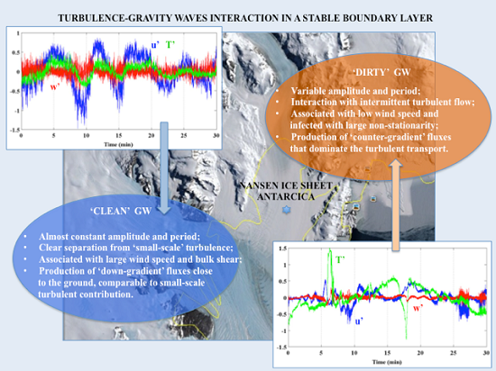
A number of studies have been concentrated on “clean” linear GWs with nearly constant amplitude and period. However, the existence of such “monochromatic” waves are rare in the SBL as most of the observed waves occur in local packets and consist of only a few cycles with changing amplitude and period. These non-stationary atmospheric wavelike disturbances, often called “dirty” waves, frequently degrade and lead to the generation of intermittent turbulence [1,17]. They are often superimposed on turbulent fluctuations and are not always clearly distinguishable from them. In those cases, separation of waves and turbulent fluctuations from time series is problematic due to the frequent absence of a defined spectral gap between the two types of motions [18,19,21].

In a recent study, Sun et al. [17] proposed an interesting interpretation of the wave-turbulence interaction that depended on both background flow and wave disturbance. Large coherent eddies can be generated by bulk shear instability triggered by the enhanced wind speed at the wave crests. The consequent increase in the turbulent mixing vertically redistributes momentum and heat and modifies the original wavy oscillations, producing apparent waves at the upper level of the mixing depth. These turbulence-forced oscillations coherently transport momentum and heat and can produce counter-gradient fluxes. Finally, GWs can generate weak turbulent mixing by enhancing the local shear instability above the wave speed troughs. The mechanisms described by Sun et al. [17] may explain the commonly observed variations in amplitude and periods of GWs and may highlight the potential role of waves in the induction of global intermittent turbulence in the SBL.

Different methods have been proposed to filter GWs in turbulence time series. In the cases of rare linear and monochromatic waves in which a spectral gap or phase relation between variables is clearly defined, the discrimination between waves and turbulence becomes possible by using wave phase averaging or band-passed filters in Fourier space [22,23,24]. However, in the frequent cases of “dirty waves”, these techniques are not effective and different methods based on multiresolution decomposition or wavelet analysis have been proposed for their localisation properties [17,25,26,27,28].

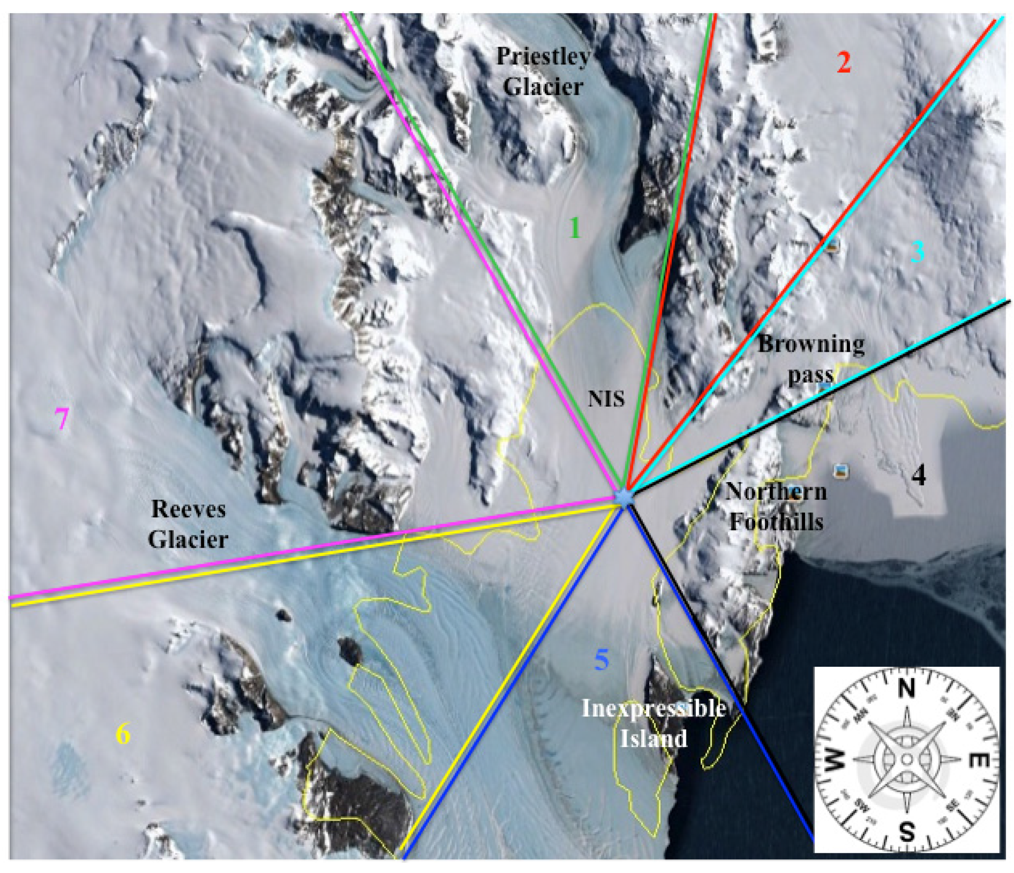
Data collected on the Nansen Ice Sheet (NIS), Antarctica, in the middle of a wide and homogeneous gently sloping area were analysed using these decompositions. Antarctica is an ideal location for exploring the characteristics of the SBL and the GWs because of persistent conditions of strong atmospheric stability in the lower troposphere. Because of their influence on tropospheric and stratospheric circulations and chemistry in the Polar region, Antarctic GWs have been the subject of several studies. These studies suggest that the GW waves are often excited by topography and by katabatic winds that flow down from the glaciers originating from the Antarctic plateau towards the coast [11,26,29,30,31,32,33,34].

The goal here is to investigate the characteristics of GWs detected on the NIS during an austral summer and to explore their impact on turbulence statistics and fluxes. A brief description of the experimental site is presented in Section 2; the methods used to identify and filter the GWs from time series are described in Section 3; and the obtained results are presented and discussed in Section 4 and Section 5.

2. Experimental Site and Instrumentation

The data analysed were sampled on the Nansen Ice Sheet (NIS) in Northern Victoria Land, Antarctica (Figure 1). The NIS is a permanently frozen branch of the Ross Sea, which penetrates for 50 km into a region surrounded by complex topography. On the arch from SW to NE, it is surrounded by mountains rapidly rising towards the Antarctic Plateau (2200 m high); from E to SE it is bordered by the Northern Foothills (600 m high); and on the S, it is confined by the open sea during the summer months. In this homogeneous and gently sloping (0.4%) area, two major glaciers converge, allowing katabatic winds to form and strongly influence the site climatology [35,36]. The Priestley glacier descends down the Antarctic Plateau from the N along a narrow, gently sloping valley; the Reeves glacier converges from the NW along a large and steep valley.

Figure 1. Satellite image of Victoria Land in West Antarctica. The star indicates the position of the micrometeorological tower located in the middle of a flat snowy homogeneous area on the Nansen Ice Sheet (NIS). The coloured lines bound the wind direction sectors used to classify the analysed data as defined in Section 3.1.

Figure 1. Satellite image of Victoria Land in West Antarctica. The star indicates the position of the micrometeorological tower located in the middle of a flat snowy homogeneous area on the Nansen Ice Sheet (NIS). The coloured lines bound the wind direction sectors used to classify the analysed data as defined in Section 3.1.

A field campaign was performed during the austral summer (from 20 November 1993 to 16 February 1994) and the micrometeorological tower was located at 74°41′58″S, 163°30′50″E, in the middle of a flat snowy homogeneous area (the star in Figure 1).

Turbulence measurements were performed at three levels (2, 4.5, and 10 m) above the surface using symmetric 3-axis ultrasonic anemometers (Gill Ins. Ltd.) Wind velocity components (u, v, w) and sonic anemometer temperature (T) were sampled at a frequency of 20.8 Hz. Fluctuations of water vapour concentration (q) were measured by a fast-response KH-20 krypton hygrometer at the highest level. Further details on the experimental campaign and the site characteristics can be found elsewhere [37,38,39].

3. Method of Analysis

3.1. Preliminary Data Processing and Selection

The preliminary step in data analysis is the detection of wavy motions in the flow. Before taking this step, the wind velocity components were rotated [40] to avoid misalignment between the instruments and the local streamlines. For this reason, a three-dimensional rotation was applied so that the horizontal wind components were aligned with the main flow and the average vertical velocity and the $\overline{v\prime w\prime }$ covariance were forced to zero. Moreover, linear trends were removed before further signal processing was conducted.

The 30-min runs were visually analysed to identify periods with apparent wavelike structures. The selected time series were classified on the basis of seven wind direction sectors (see Figure 1). Sector 1 (330°–10°) corresponds to frequent and persistent drainage winds along the Priestley glacier with variable intensities; Sector 2 (10°–45°) corresponds to winds perturbed by local orography (maximum height ~1800 m); Sector 3 (45°–60°) corresponds to frequent drainage winds from the Browning pass (an ice-covered pass, 19 km long, maximum height ~600 m); Sector 4 (60°–150°) corresponds to winds topographically perturbed by the Northern Foothills (a line of coastal hills with a maximum height ~800 m); Sector 5 (150°–210°) corresponds to winds essentially flowing from the sea, and in some cases locally perturbed by Inexpressible Island (a 300-m high ridge); Sector 6 (210°–260°) corresponds to katabatic winds of variable intensities along the Reeves glacier; Sector 7 (260°–330°) corresponds to winds perturbed by local orography rapidly rising towards the Antarctic Plateau (~2200 m high). The characteristics of the selected wavy structures and their interaction with turbulence were investigated using the methodologies described in the following section.

3.2. Identification and Filtering of Wave Activity

The nature of the wavy patterns identified in the selected runs was explored using the spectral and cross-spectral analysis of the wind velocity components and scalars. The cospectral indicators allow the discrimination between the linear waves and other “dirty” waves when mixed with turbulence that may contribute to the transport of passive tracers.

Hereafter, an overbar indicates time averaging over a 30-min interval and a prime denotes fluctuation from the 30-min time average. Briefly, the cross-spectrum between two variables (a, b) is the Fourier Transform of their cross-correlation function [41]. Its real part is designated as the cospectrum (C_ab) and its integral represents the covariance $\overline{a\prime b\prime }$; its imaginary part (Q_ab) is designated as the quadspectrum (or quadrature spectrum) and represents the spectrum of the product of a and b shifted by 90°. Moreover the phase spectrum, defined as

ϕ_ab (f)= tan⁻¹ (Q_ab (f) /C_ab (f))

(1)

represents the phase difference between the a and b time series that yields the greatest correlation for each natural frequency f (in Hz).

The chaotic and diffusive character approximating turbulent exchange causes a peak in the cospectrum of vertical velocity and scalars in the energy-containing region. In this range of frequencies, the quadspectrum is usually small and the phase spectrum is randomly distributed between −π and +π, resulting in a mean value close to zero. In the presence of linear waves, the lack of vertical diffusion produces fluctuations of vertical velocity and scalars 90° out of phase. Therefore, in the wave source region, the quadspectrum is larger than the cospectrum and the phase spectrum assumes values close to ±90°.

In summary, cospectral indicators are used to initially identify the frequencies associated with wave events in the measured series. Then, the detected frequencies can be exploited to separate waves from the turbulent fluctuations in the time series of wind components and scalars using a multiresolution (MR) decomposition based on the Haar wavelet (localised in the time domain).

MR analysis orthogonally decomposes the series into averages on different time scales and at each step acts as a high-pass filter that removes increasingly shorter averaging timescale components. Further details on the MR decomposition technique can be found elsewhere [42,43,44,45].

Each mode of the MR decomposition satisfies the rules of Reynolds averaging, which is a departure from the global Fourier transform. For this reason and for its localisation properties, MR analysis is often applied to correctly evaluate turbulent statistics and fluxes by filtering contamination from non-turbulent contributions such as wavelike perturbations. The original unfiltered signal (x) can be decomposed into three components:

$$x=\overline{x}+\tilde{x}+x\prime$$

(2)

where $\overline{x}$ represents the global mean value, $\tilde{x}$ represents the wavy perturbation and $x\prime$ represents the true turbulent fluctuation.

Using this triple decomposition, unfiltered turbulent statistics and fluxes computed by using the original fluctuations $\left(x-\overline{x}\right)$ can be compared to a version computed using the wave corrected fluctuations $\left(x-\overline{x}-\tilde{x}\right)$ to assess the effects of wavelike structures on turbulence parameters.

Both spectral and wavelet analyses were conducted on runs of 32,768 data points and, thus, the resolved frequency bandwidth ranged from 0.0005 Hz to 10.4 Hz.

4. Results

To address the study objectives, the presence of wavy structures in each 30-min time series of velocity components and scalars was identified visually. In this first step, data sampled at the highest level (10 m) was used for guidance because the wavy patterns appeared more definite at this level when compared with the two lower levels (4.5 m and 2 m). This is consistent with the observations of Sun et al. [17] and it is due to the decreasing influence of turbulence mixing on GWs with height [17,46]. Wavelike motion was observed on most of the 55 days analysed within the SBL. However, only some 80 runs exhibited a discernable wavy pattern as identified and confirmed by the spectral and cospectral analyses. Table 1 summarises the number and percentage of detected events classified on the basis of the wind direction sectors defined in Section 3.1. It is evident that the wavy events appear to be associated with winds originating from inland (in particular from Sectors 1 and 3). These waves are probably “excited” by orography or by katabatic winds blowing from the Antarctic Plateau towards the coast as previously reported in other studies [11,26,29,30,31,32,33,34]. Moreover, the detected waves were observed during moderate or low wind conditions where the mean velocity (U) at a 10-m height did not exceed 4 m·s⁻¹.

Table 1. Classification of the selected 30-min time series based on different wind direction sectors (see Figure 1). N refers to the number of runs exhibiting a wavelike pattern; (%)_TOT and (%)_GW refer to the percentage of runs exhibiting a wavy pattern relative to the total number of runs in each sector and relative to the total cases of GW, respectively; U represents the average mean wind associated with the wavy selected events for each sector at z = 10 m.

Sectors	1	2	3	4	5	6	7
Wind direction (°)	330–10	10–35	45–60	60–150	150–210	210–260	260–330
N	19	13	19	5	11	1	12
(%)TOT	8.0	9.0	6.8	1.8	3.2	0.9	4.9
(%)GW	23.8	16.2	23.8	6.2	13.8	1.2	15.0
U (m·s−1)	2.3 ± 1.6	3.0 ± 0.9	2.2 ± 1.1	2.1 ± 1.7	2.4 ± 1.7	2.3	2.2 ± 1.5

Table 1. Classification of the selected 30-min time series based on different wind direction sectors (see Figure 1). N refers to the number of runs exhibiting a wavelike pattern; (%)_TOT and (%)_GW refer to the percentage of runs exhibiting a wavy pattern relative to the total number of runs in each sector and relative to the total cases of GW, respectively; U represents the average mean wind associated with the wavy selected events for each sector at z = 10 m.

Sectors	1	2	3	4	5	6	7
Wind direction (°)	330–10	10–35	45–60	60–150	150–210	210–260	260–330
N	19	13	19	5	11	1	12
(%)TOT	8.0	9.0	6.8	1.8	3.2	0.9	4.9
(%)GW	23.8	16.2	23.8	6.2	13.8	1.2	15.0
U (m·s−1)	2.3 ± 1.6	3.0 ± 0.9	2.2 ± 1.1	2.1 ± 1.7	2.4 ± 1.7	2.3	2.2 ± 1.5

The detected wavelike structures were rarely monochromatic (with constant amplitude and period), but appeared as multiple events that persisted only for a few cycles with variable amplitudes and periods as observed elsewhere [1,17,20]. Often, the propagation of these “dirty” waves produced non-stationarity and strong global intermittency in turbulent fluctuations.

Figure 2. Time series of longitudinal (a) and vertical velocity components (b), sonic anemometer air temperature (c) and fluctuations in water vapour concentration (d) for a selected but uncommon case of a “cleaner” wave (Wave 1). The time series were collected on the 24 November 1993 at 18:00 (local time) and were associated with a drainage wind from the Priestley glacier (Sector 1). The different colours refer to the different levels of measurement: red (10 m), green (4.5 m), blue (2 m). The black dashed lines refer to the mean values. Note that in Figure 2a,b, the time series relative to the lowest levels (green and blue lines) have been artificially shifted for better visualisation purposes.

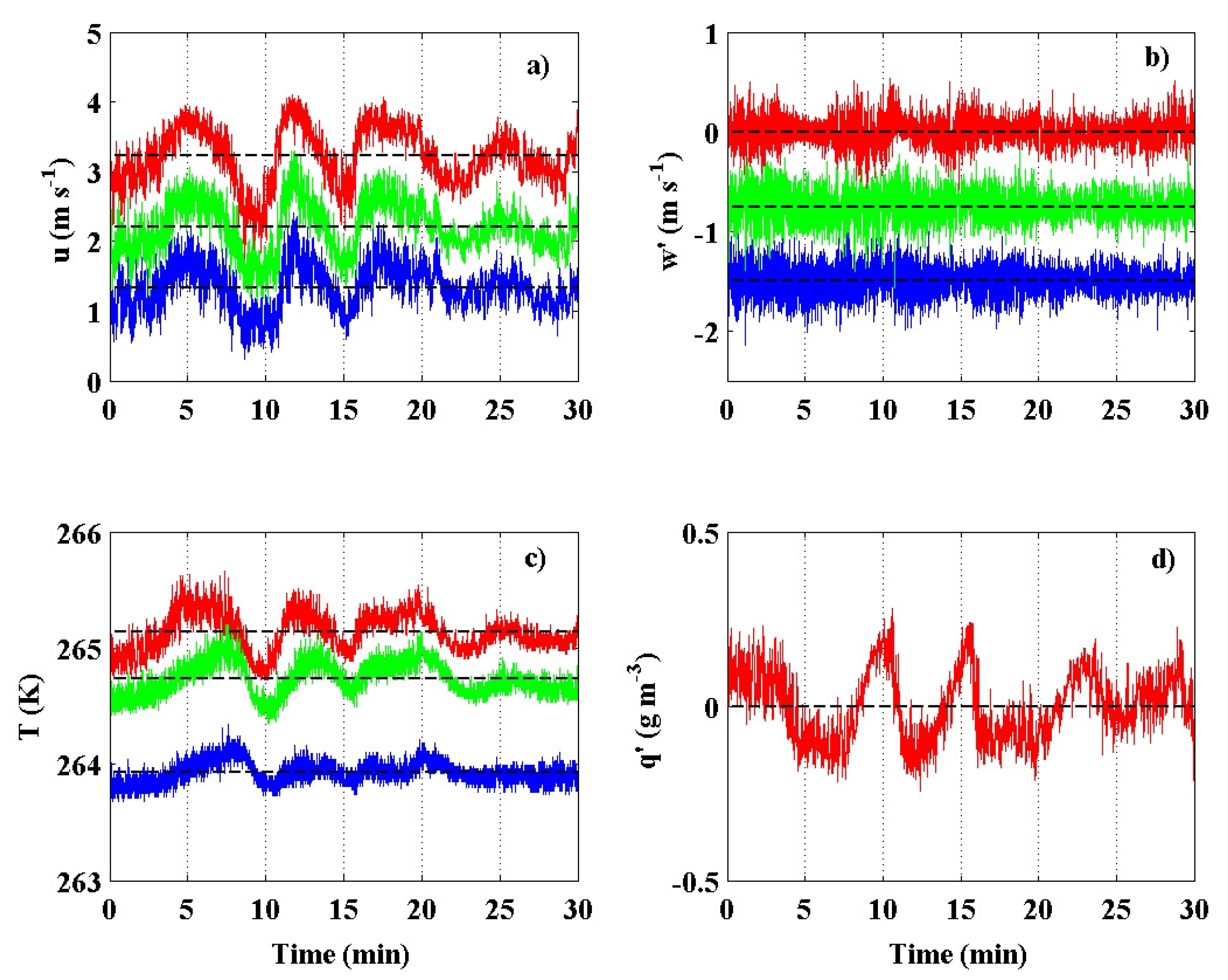
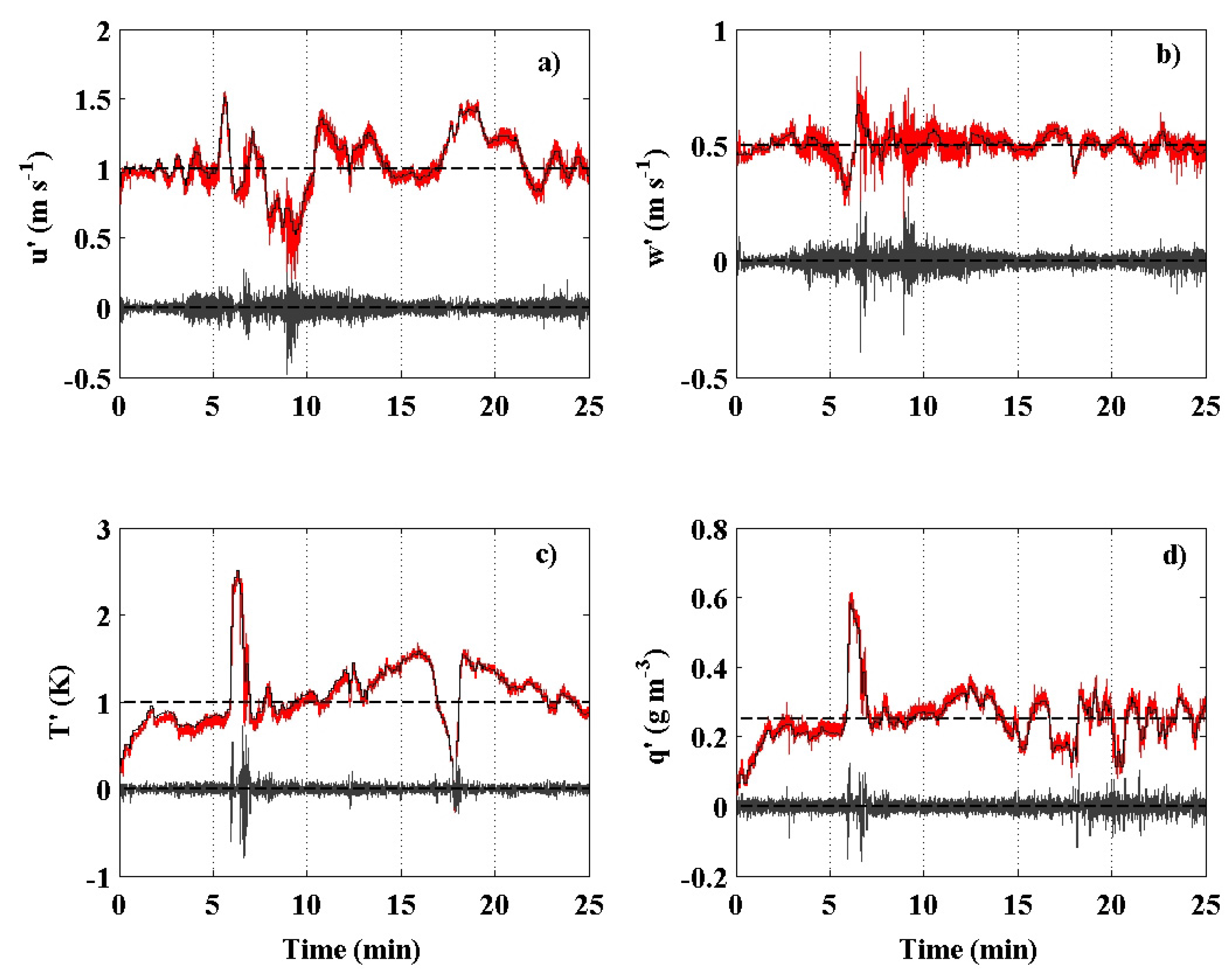
Figure 2. Time series of longitudinal (a) and vertical velocity components (b), sonic anemometer air temperature (c) and fluctuations in water vapour concentration (d) for a selected but uncommon case of a “cleaner” wave (Wave 1). The time series were collected on the 24 November 1993 at 18:00 (local time) and were associated with a drainage wind from the Priestley glacier (Sector 1). The different colours refer to the different levels of measurement: red (10 m), green (4.5 m), blue (2 m). The black dashed lines refer to the mean values. Note that in Figure 2a,b, the time series relative to the lowest levels (green and blue lines) have been artificially shifted for better visualisation purposes.

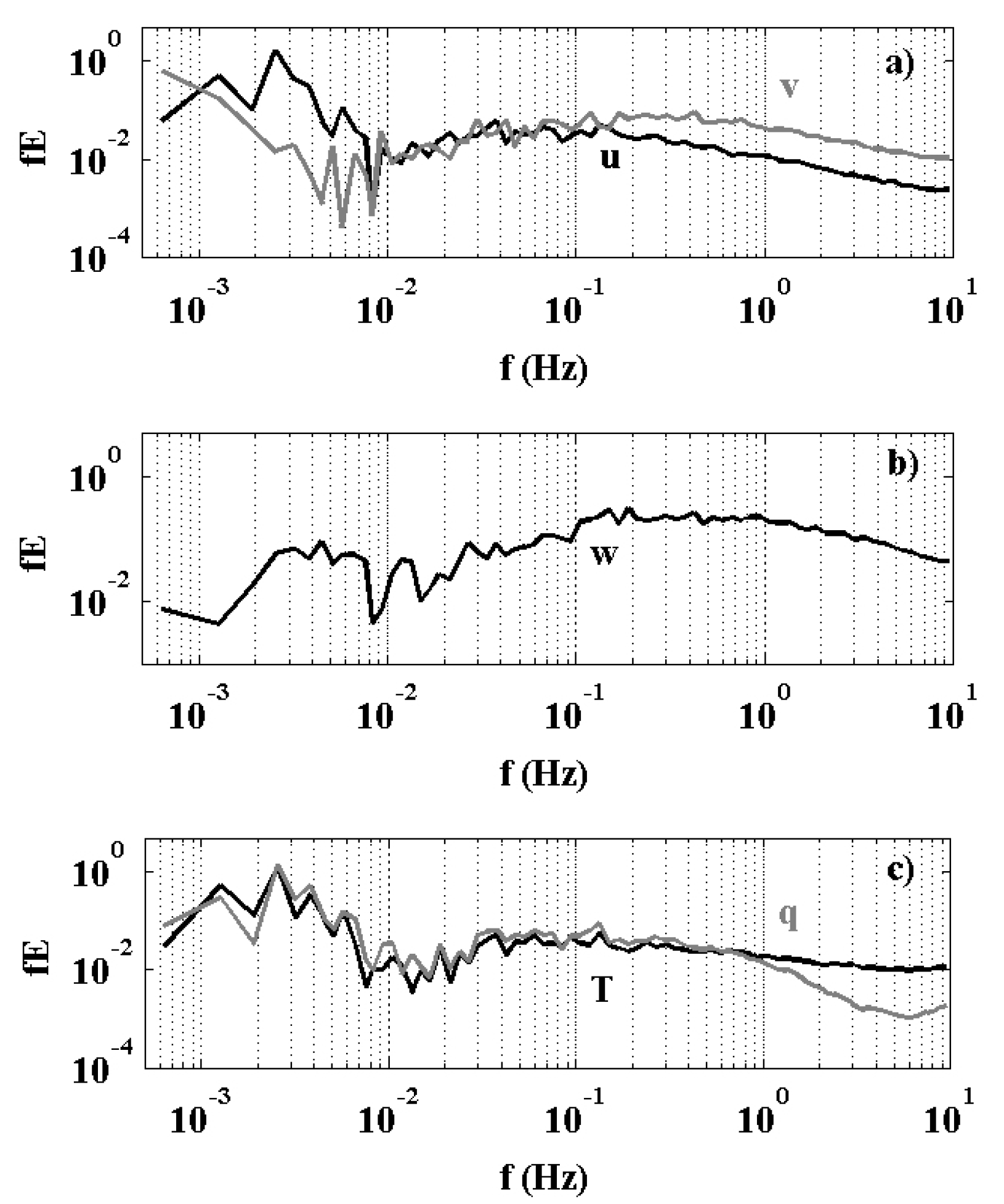
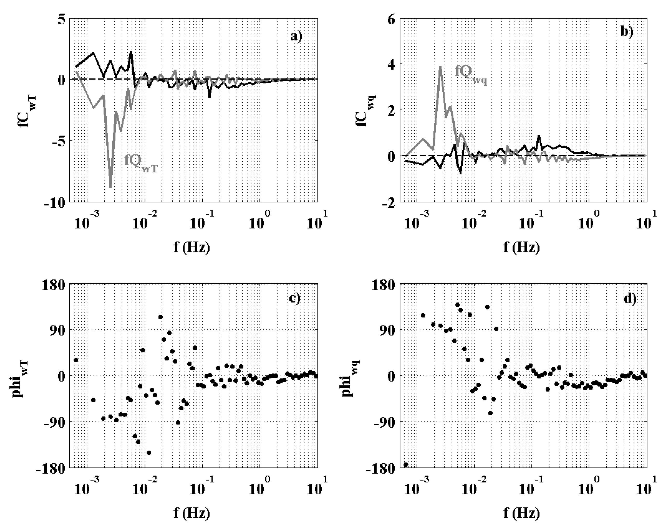
Figure 2 and Figure 3 feature two examples of wavy events in the records. Figure 2 displays a case of a roughly “clean” wave characterised by a period of about 6–7 minutes (hereafter Wave 1). It is associated with a decelerating phase of a moderate drainage wind from the Priestley glacier (Sector 1). The stationarity indices based on different stationarity tests (RN: [47]; NR: [48]; I_C: [9]) were computed at the highest level for sensible heat flux (RN = 28, NR = 0.9, I_C = 1) and latent heat flux (RN = 8, NR = 0.9, I_C = 1), indicating stationarity of the corresponding time series. The period and amplitude of the wave changed slightly during the analysed episode. Moreover, the wave period did not differ at the three measurement heights even if the amplitude tended to be attenuated closer to the ice sheet surface. This is mainly true for the vertical velocity component that is characterised by smaller wave amplitude superimposed onto increasing levels of turbulence activity near the ground. Spectral and cospectral analyses (Figure 4 and Figure 5) further highlight the presence of a well-defined spectral gap between the turbulence and the wave frequency range. In fact, the spectra of the wind components and the scalars exhibited a secondary maximum at f~0.0025 Hz, corresponding to the same wave period observed in the time series (6–7 minutes). This low frequency maximum is well separated from the turbulence frequency range by a gap at f~0.01 Hz. At the frequency of the wave maximum quadspectra, the phase spectrum approaches −90° for w-T cross-spectrum and +90° for the w-q cross-spectrum, indicating the small diffusive characteristic of this detected wave.

Figure 3. As per Figure 2 but for a selected case of a “dirty” wave (Wave 2). The time series were collected on 28 December 1993 at 00:30 (local time) and were associated with a drainage wind originating from the Browning pass (Sector 3).

Figure 3. As per Figure 2 but for a selected case of a “dirty” wave (Wave 2). The time series were collected on 28 December 1993 at 00:30 (local time) and were associated with a drainage wind originating from the Browning pass (Sector 3).

Figure 3 displays an example of a “dirty” wave characterised by variable amplitude and period and by an evident interaction with turbulent flow, highlighted by localised gustiness in turbulent fluctuations (hereafter Wave 2). This event occurred during a light drainage wind originating from the Browning pass (Sector 3). For this wavy episode, the stationarity indices at the highest level for sensible heat flux were RN = 41, NR = 1.7, I_C = 0.87, and for latent heat flux were RN = 31, NR = 1.7, I_C = 0.91 indicating a weaker stationarity of the corresponding time series with respect to the case shown in Figure 2 (Wave 1).

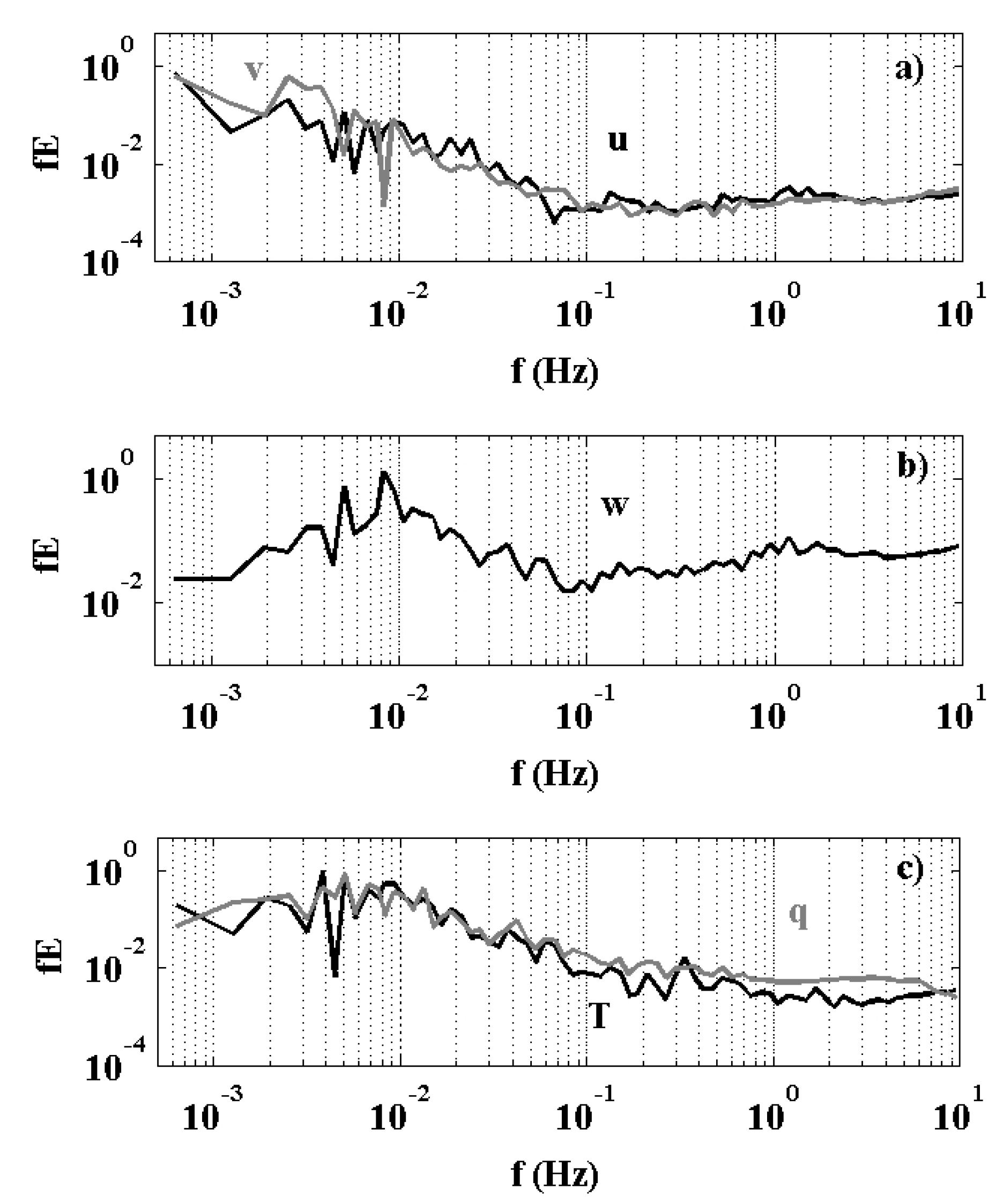
Figure 4. Spectra (in pre-multiplied form) computed for the longitudinal and lateral wind velocity components (a), for vertical wind component (b) and for temperature and water vapour (c) versus the natural frequency (f) relative to the time series shown in Figure 2 and sampled at the highest level (10 m).

Figure 4. Spectra (in pre-multiplied form) computed for the longitudinal and lateral wind velocity components (a), for vertical wind component (b) and for temperature and water vapour (c) versus the natural frequency (f) relative to the time series shown in Figure 2 and sampled at the highest level (10 m).

Figure 5. Cospectra (black lines) and quadrature spectra (grey lines) for the w-T cross-spectrum (a) and the w-q cross-spectrum (b); phase spectra for the w-T cross-spectrum (c) and the w-q cross-spectrum (d) versus the natural frequency (f) relative to the time series shown in Figure 2 and sampled at the highest level (10 m).

Figure 5. Cospectra (black lines) and quadrature spectra (grey lines) for the w-T cross-spectrum (a) and the w-q cross-spectrum (b); phase spectra for the w-T cross-spectrum (c) and the w-q cross-spectrum (d) versus the natural frequency (f) relative to the time series shown in Figure 2 and sampled at the highest level (10 m).

Figure 6. As per Figure 4 but relative to the time series shown in Figure 3.

Figure 6. As per Figure 4 but relative to the time series shown in Figure 3.

Figure 7. As per Figure 5 but relative to the time series shown in Figure 3.

Figure 7. As per Figure 5 but relative to the time series shown in Figure 3.

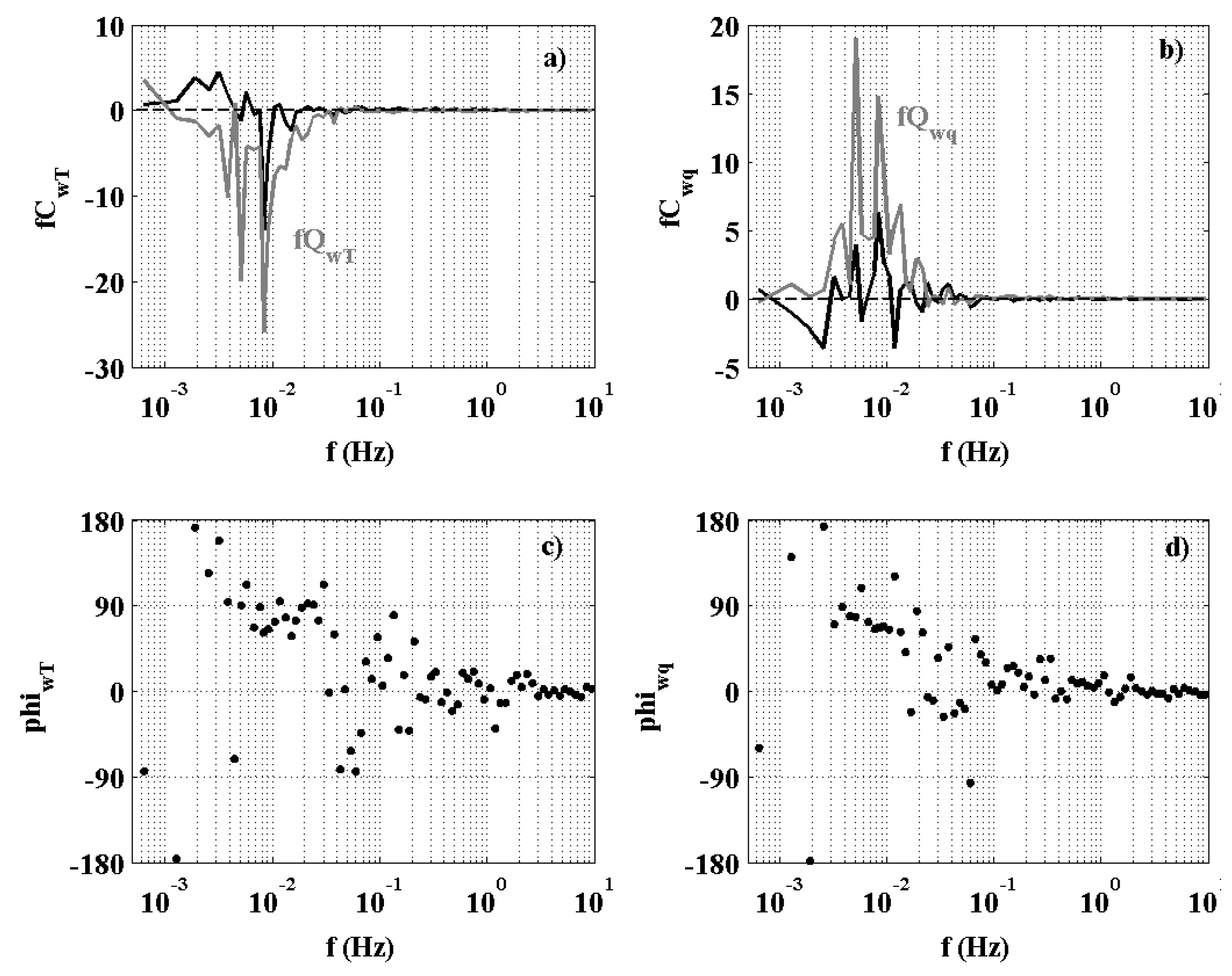
Again, the wavy pattern and amplitude appear attenuated closer to the surface, but more accentuated than in the previous example shown in Figure 2. Spectral and cospectral analyses (Figure 6 and Figure 7) suggest a “quasi-chaotic” behaviour of the analysed wavy episode. In fact, in the wave frequency range [0.003 ÷ 0.02], both spectra and the quadrature spectra exhibit multiple peaks and the scalar cospectra display an erratic behaviour with flux fluctuations of varying signs (signature of counter-gradient fluxes). Despite this behaviour, a spectral gap between wave and turbulent motions can be identified at f~0.1 Hz.

Figure 8. Triple decomposition of longitudinal (a) and vertical wind velocity components (b), sonic anemometer temperature (c) and water vapour concentration (d) relative to the case of the “cleaner” gravity wave shown in Figure 2 (Wave 1) and sampled at the highest level (10 m). The time series were filtered using the MR decomposition technique based on the Haar wavelet. The threshold frequency used to separate wavy and turbulent components (f~0.01 Hz) was selected on the basis of the spectral analyses shown in Figure 4 and Figure 5. The red lines represent the original fluctuations $\left(x-\overline{x}\right)$, the black lines represent the filtered wavy components $\left(\tilde{x}\right)$, and the grey lines represent the wave-corrected fluctuations $\left(x-\overline{x}-\tilde{x}\right)$. Note that red lines have been artificially shifted for better visualisation purposes.

Figure 8. Triple decomposition of longitudinal (a) and vertical wind velocity components (b), sonic anemometer temperature (c) and water vapour concentration (d) relative to the case of the “cleaner” gravity wave shown in Figure 2 (Wave 1) and sampled at the highest level (10 m). The time series were filtered using the MR decomposition technique based on the Haar wavelet. The threshold frequency used to separate wavy and turbulent components (f~0.01 Hz) was selected on the basis of the spectral analyses shown in Figure 4 and Figure 5. The red lines represent the original fluctuations $\left(x-\overline{x}\right)$, the black lines represent the filtered wavy components $\left(\tilde{x}\right)$, and the grey lines represent the wave-corrected fluctuations $\left(x-\overline{x}-\tilde{x}\right)$. Note that red lines have been artificially shifted for better visualisation purposes.

Spectral and cospectral analyses were applied to the 80 selected runs to detect the frequency ranges of the wavy structures and the associated spectral gaps. Next, the time series of the wind components and scalars were filtered out by using the MR decomposition based on the Haar wavelet to separate waves from turbulent fluctuations. Figure 8 and Figure 9 show the triple decomposition of the measured time series obtained as a result of the MR filtering methodology applied to the wavy events shown in Figure 2 and Figure 3. It is evident that the wave passage coincides with the production of large and intermittent turbulent fluctuations, in particular in the case of Wave 2 (Figure 9).

Figure 9. As per Figure 8, but for the case of the “dirty” wave shown in Figure 3 (Wave 2). The threshold frequency used to separate the wavy and turbulent components (f~0.1 Hz) was chosen on the basis of the spectral analyses shown in Figure 6 and Figure 7.

Figure 9. As per Figure 8, but for the case of the “dirty” wave shown in Figure 3 (Wave 2). The threshold frequency used to separate the wavy and turbulent components (f~0.1 Hz) was chosen on the basis of the spectral analyses shown in Figure 6 and Figure 7.

Figure 10. Scatter plot of unfiltered turbulent statistics versus the same statistics corrected for the wave effect: standard deviation of the longitudinal (a), lateral (b) and vertical wind velocity component (c), and friction velocity (d). The different colours and symbols refer to the different levels of measurement: red stars (10 m), green points (4.5 m), blue diamonds (2 m). Coloured dotted lines represent the linear best-fit regression lines whereas the black dotted line represents the 1:1 line.

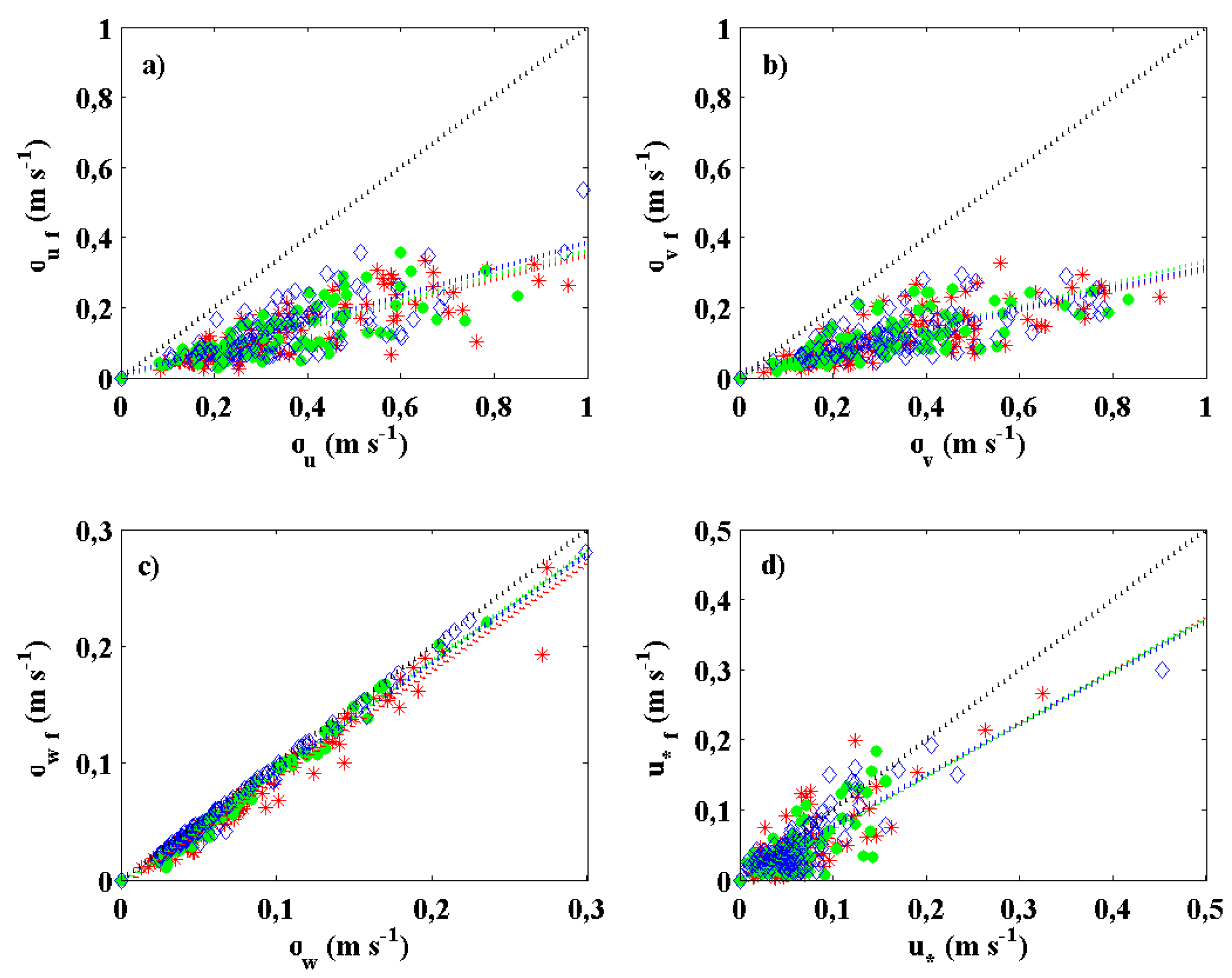
Figure 10. Scatter plot of unfiltered turbulent statistics versus the same statistics corrected for the wave effect: standard deviation of the longitudinal (a), lateral (b) and vertical wind velocity component (c), and friction velocity (d). The different colours and symbols refer to the different levels of measurement: red stars (10 m), green points (4.5 m), blue diamonds (2 m). Coloured dotted lines represent the linear best-fit regression lines whereas the black dotted line represents the 1:1 line.

The obtained triple decomposition was used to compare the turbulent statistics and fluxes computed using the original fluctuations $\left(x-\overline{x}\right)$ and the turbulence fluctuations after the wave effects were filtered out $\left(x-\overline{x}-\tilde{x}\right)$ (Figure 10 and Figure 11). Table 2 and Table 3 contain the result of the linear regression analysis reported in Figure 10 and Figure 11, respectively. Unsurprisingly, these results suggest that the inclusion of wavy oscillations produce an overestimate of the variances associated with turbulence. The impact of waves appears to be similar at all the measurement heights even if the fractional contribution changes for the different turbulent statistics. As observed elsewhere [18], one of the statistics more impacted by the waves is the turbulent kinetic energy (TKE) and, in particular, the longitudinal and lateral contributions. In fact, the wave filtering produced a reduction of more than 60% in σ_u and σ_v with respect to the unfiltered values (Figure 10a,b). On the other hand, σ_w slightly decreased after the wave filtering (less than 10%) (Figure 10c), suggesting that the pancake nature of eddies in a highly stratified SBL flow may be linked to some wave effects. A large wave impact was also observed in the standard deviations of the scalars that appear to be reduced by about 50%–60% (Figure 11a,b), commensurate with σ_u and σ_v.

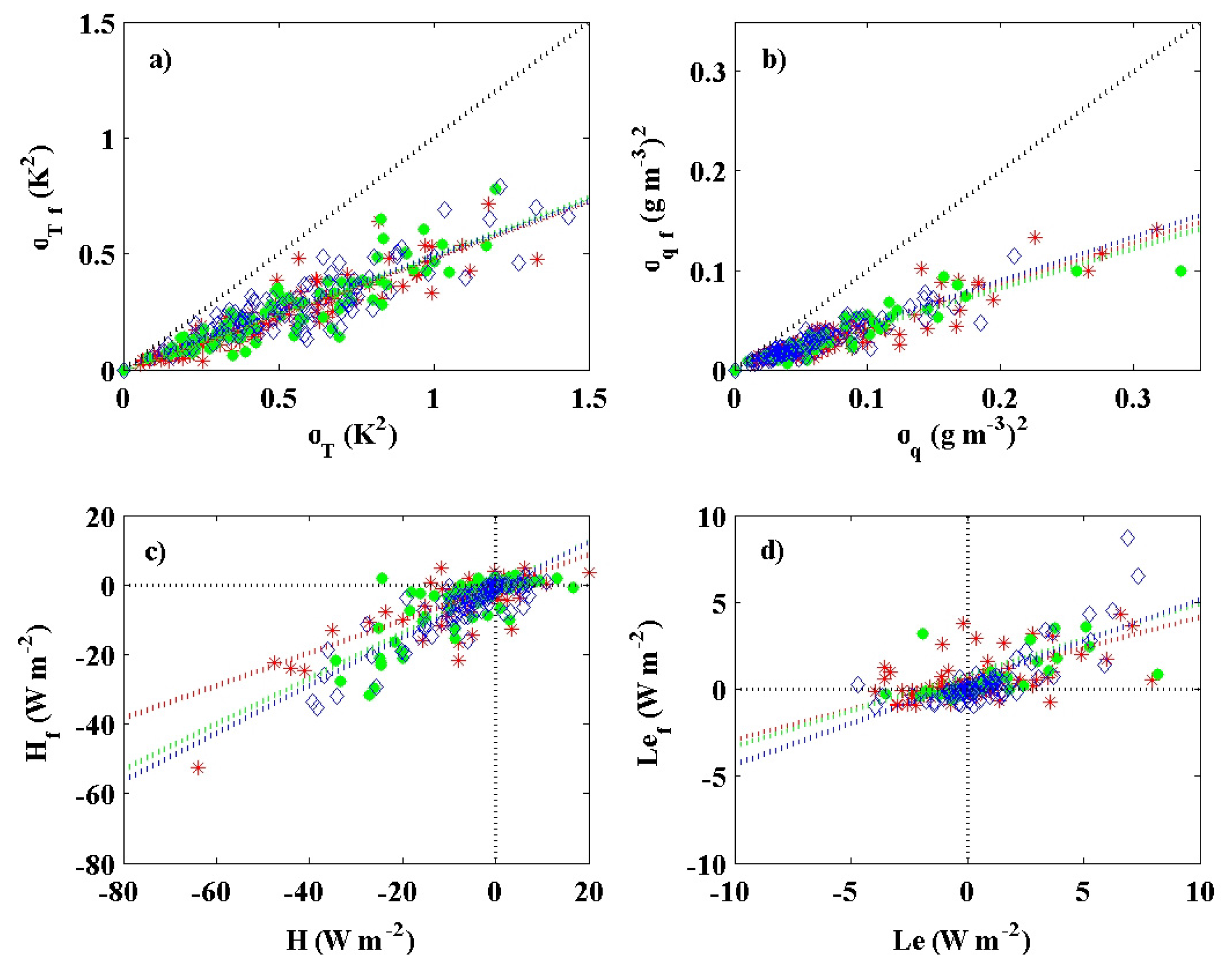
Figure 11. Same as Figure 10 but for the standard deviation of air temperature (a) and water vapour (b), sensible heat flux (c), and latent heat flux (d).

Figure 11. Same as Figure 10 but for the standard deviation of air temperature (a) and water vapour (b), sensible heat flux (c), and latent heat flux (d).

The effect of wave activity on momentum and scalar fluxes is more complex compared with the variances (the presence of waves always increases the overall variance). In fact, waves can produce large errors in sign and magnitude of the computed turbulent fluxes [14] or they themselves can contribute to intermittent turbulent mixing [17].

As an example, Table 4 displays the different contributions of the wavy and turbulent fluctuations to the total fluxes of momentum and sensible heat relative to the time series shown in Figure 2 and Figure 3. In both episodes, waves can produce counter-gradient fluxes, which was also reported by Sun et al. [17]. However in the case of Wave 1 experiencing larger mean wind speed and bulk shear, the wave resulted in strong mixing and produced down-gradient fluxes at the lower levels comparable to those associated with small-scale turbulent fluctuations. On the other hand, Wave 2 was associated with a lower wind speed and a larger non-stationarity; as a consequence, counter-gradient fluxes were also measured at the lowest level, and wave contributions appeared to dominate the total transport due the low levels of small-scale turbulence. These patterns are consistent with the cospectra shown in Figure 5 and Figure 7

Table 2. Linear regression analysis of turbulent statistics and fluxes computed by using the original fluctuations and corrected for the wave effect shown in Figure 10. The subscribed numbers refer to different levels of measurements (1 → 10 m; 2 → 4.5 m; 3 → 2 m). R² is the coefficient of determination associated with the regression analysis.

Linear Fit	R2
σu1f = 0.34 σu1 + 0.01	0.75
σu2f = 0.36 σu2 + 0.00	0.75
σu3f = 0.38 σu3 + 0.00	0.73
σv1f = 0.29 σv1 + 0.02	0.64
σv2f = 0.32 σv2 + 0.01	0.75
σv3f = 0.30 σv3 + 0.02	0.71
σw1f = 0.92 σw1 - 0.01	0.98
σw2f = 0.95 σw2 + 0.00	0.99
σw3f = 0.93 σw3 + 0.00	0.98
u*1f = 0.75 u*1 + 0.00	0.64
u*2f = 0.75 u*2 + 0.00	0.63
u*3f = 0.73 u*3 + 0.00	0.80

Table 2. Linear regression analysis of turbulent statistics and fluxes computed by using the original fluctuations and corrected for the wave effect shown in Figure 10. The subscribed numbers refer to different levels of measurements (1 → 10 m; 2 → 4.5 m; 3 → 2 m). R² is the coefficient of determination associated with the regression analysis.

Linear Fit	R2
σu1f = 0.34 σu1 + 0.01	0.75
σu2f = 0.36 σu2 + 0.00	0.75
σu3f = 0.38 σu3 + 0.00	0.73
σv1f = 0.29 σv1 + 0.02	0.64
σv2f = 0.32 σv2 + 0.01	0.75
σv3f = 0.30 σv3 + 0.02	0.71
σw1f = 0.92 σw1 - 0.01	0.98
σw2f = 0.95 σw2 + 0.00	0.99
σw3f = 0.93 σw3 + 0.00	0.98
u*1f = 0.75 u*1 + 0.00	0.64
u*2f = 0.75 u*2 + 0.00	0.63
u*3f = 0.73 u*3 + 0.00	0.80

Table 3. Same as Table 2 but for turbulent statistics and fluxes computed using the original fluctuations and corrected for the wave effect, shown in Figure 11.

Linear Fit	R2
σT1f = 0.49 σT1 − 0.01	0.92
σT2f = 0.50 σT2 + 0.00	0.87
σT3f = 0.48 σT3 + 0.01	0.85
σq1f = 0.42 σq1 + 0.00	0.85
σq2f = 0.40 σq2 + 0.00	0.92
σq3f = 0.44 σq3 + 0.00	0.88
H1f = 0.47 H1 − 0.76	0.67
H2f = 0.66 H2 − 0.67	0.68
H3f = 0.69 H3 − 1.53	0.78
Le1f = 0.35 Le1 + 0.60	0.45
Le2f = 0.41 Le2 + 0.80	0.53
Le3f = 0.48 Le3 + 0.38	0.46

Table 3. Same as Table 2 but for turbulent statistics and fluxes computed using the original fluctuations and corrected for the wave effect, shown in Figure 11.

Linear Fit	R2
σT1f = 0.49 σT1 − 0.01	0.92
σT2f = 0.50 σT2 + 0.00	0.87
σT3f = 0.48 σT3 + 0.01	0.85
σq1f = 0.42 σq1 + 0.00	0.85
σq2f = 0.40 σq2 + 0.00	0.92
σq3f = 0.44 σq3 + 0.00	0.88
H1f = 0.47 H1 − 0.76	0.67
H2f = 0.66 H2 − 0.67	0.68
H3f = 0.69 H3 − 1.53	0.78
Le1f = 0.35 Le1 + 0.60	0.45
Le2f = 0.41 Le2 + 0.80	0.53
Le3f = 0.48 Le3 + 0.38	0.46

The effect of wave filtering on momentum and scalar fluxes in all the selected episodes is reported in Figure 11c,d. As already observed elsewhere (i.e., [14]), the friction velocity u_* appears reduced after the wave filtering (by about 25%). The waves have a larger impact on the turbulent fluxes of scalars. Figure 11 confirms that waves often produce counter-gradient positive values of sensible heat flux (H). In reality, the surface H should be negative in a stably stratified boundary layer experiencing wavy motion. The wave filtering corrects the turbulent H sign (that becomes negative), but the magnitude is reduced (also as expected for weak turbulence conditions). On the other hand, in the negative quadrant (H < 0 and H_f < 0) where both unfiltered and filtered fluxes are negative, the filtered flux appears less negative than the uncorrected total flux. The percentage of sensible heat flux magnitude reduction due to filtering apparently increased with increasing measurement height (from 30% at 2 m to 50% at 10 m), as reported in Table 3.

Table 4. Wind speed (U) and contributions of the wavy and turbulent fluctuations to the total fluxes of momentum ($\overline{u\prime w\prime }$) and sensible heat (H) relative to the time series shown in Figure 2 (Wave 1) and Figure 3 (Wave 2) at the three measurement heights. Values in bold and underlined characters indicate counter-gradient fluxes.

Wave 1
Height	10	4.5	2
U (m·s−1)	3.2	2.5	2.3
$\overline{u\prime w\prime }$ (m·s−1)2
total wave turbulence	−0.7 × 10−3 +3.6 × 10−3 −4.3 × 10−3	−12.0 × 10−3 −7.0 × 10−3 −7.0 × 10−3	−16.0 × 10−3 −8.0 × 10−3 −8.0 × 10−3
H (W·m−2)
total wave turbulence	−1.0 +0.5 −1.5	−6.7 −3.3 −3.4	−1.5 −0.7 −0.7
Wave 2
Height	10	4.5	2
U (m·s−1)	1.9	1.5	1.1
$\overline{u\prime w\prime }$ (m·s−1)2
total wave turbulence	−6.3 × 10−4 −5.9 × 10−4 −0.4 × 10−4	−6.7 × 10−4 −5.0 × 10−4 −1.7 × 10−4	+8.0 × 10−4 +9.7 × 10−4 −1.7 × 10−4
H (W·m−2)
total wave turbulence	+1.6 +1.7 −0.1	−8.6 −7.7 −0.9	+3.9 +4.7 −0.8

Table 4. Wind speed (U) and contributions of the wavy and turbulent fluctuations to the total fluxes of momentum ($\overline{u\prime w\prime }$) and sensible heat (H) relative to the time series shown in Figure 2 (Wave 1) and Figure 3 (Wave 2) at the three measurement heights. Values in bold and underlined characters indicate counter-gradient fluxes.

Wave 1
Height	10	4.5	2
U (m·s−1)	3.2	2.5	2.3
$\overline{u\prime w\prime }$ (m·s−1)2
total wave turbulence	−0.7 × 10−3 +3.6 × 10−3 −4.3 × 10−3	−12.0 × 10−3 −7.0 × 10−3 −7.0 × 10−3	−16.0 × 10−3 −8.0 × 10−3 −8.0 × 10−3
H (W·m−2)
total wave turbulence	−1.0 +0.5 −1.5	−6.7 −3.3 −3.4	−1.5 −0.7 −0.7
Wave 2
Height	10	4.5	2
U (m·s−1)	1.9	1.5	1.1
$\overline{u\prime w\prime }$ (m·s−1)2
total wave turbulence	−6.3 × 10−4 −5.9 × 10−4 −0.4 × 10−4	−6.7 × 10−4 −5.0 × 10−4 −1.7 × 10−4	+8.0 × 10−4 +9.7 × 10−4 −1.7 × 10−4
H (W·m−2)
total wave turbulence	+1.6 +1.7 −0.1	−8.6 −7.7 −0.9	+3.9 +4.7 −0.8

In addition, the latent heat flux appears to be attenuated by the filtering processes (Figure 11d). In these cases, the turbulent component of the latent heat flux assumes low values commonly associated with large random errors that de-correlate the water vapour fluctuations from vertical velocity fluctuations.

Finally, Figure 12 shows the wavelength of the detected waves versus the atmospheric stability parameter (z/L, where z is the measurement height and L is the Obukhov length), measured at the highest level and computed after wave filtering. Different colours and symbols refer to data belonging to different wind direction sectors. The highest values of GW wavelength correspond to weak stable stratification (z/L <1) and are of the order of a few kilometres (~1000–2000 m) as frequently observed in Antarctic coastal areas [33]. When stability increases, the wavelengths rapidly decrease and can assume extremely small values (~100 m) for strong stability conditions. For reference, exponential and power regression fits were computed and are reported in Figure 12, even if they are probably dependent on the site and topographic characteristics.

Figure 12. Wavelength of detected waves (GW) versus the atmospheric stability parameter (z/L, where z is the measurement height and L is the Obukhov length), measured at the highest level (=10 m) and computed after the wave-filtering process. Different colours and symbols refer to data belonging to different wind direction sectors. The continuous black line refers to the exponential regression: y = 1287 e^(−0.56x) (R² = 0.64); the dashed and dotted black lines refer to the power-law regressions: y = 592 x^−0.47 (R² = 0.47) and y = 5687 x^−0.06 − 5018 (R² = 0.62), respectively.

Figure 12. Wavelength of detected waves (GW) versus the atmospheric stability parameter (z/L, where z is the measurement height and L is the Obukhov length), measured at the highest level (=10 m) and computed after the wave-filtering process. Different colours and symbols refer to data belonging to different wind direction sectors. The continuous black line refers to the exponential regression: y = 1287 e^(−0.56x) (R² = 0.64); the dashed and dotted black lines refer to the power-law regressions: y = 592 x^−0.47 (R² = 0.47) and y = 5687 x^−0.06 − 5018 (R² = 0.62), respectively.

5. Conclusions

The characteristics of wavy motion and their impact on turbulent statistics, including turbulent fluxes, were investigated using measured wind velocity components and scalars collected on the NIS, Antarctica. The measurements reveal states of persistently strong atmospheric stable stratification and hence constitute ideal conditions for investigating the GW characteristics. Based on the analysis here, the following conclusions can be drawn:

-

Wavelike motions on the NIS were probably excited by the complex topography surrounding the area, as frequently observed in the Antarctic coastal regions. In fact, the detected waves were prevalently associated with moderate or low drainage winds from inland towards the coast. During conditions of weak atmospheric stratification (z/L < 1), the wavelengths were of the order of a few kilometres (1000–2000 m), comparable to the height of the surrounding orography. When stability increased, the GW wavelengths rapidly decreased and assumed extremely small values (~100 m) for strong stability conditions.

-

The observed wavy patterns were seldom monochromatic. They were frequently characterised by variable amplitude and period and persisted only for few cycles in the time series. The wave period remained unchanged with the measurement heights, but the pattern and amplitude tended to be attenuated closer to the ground surface due to the increasing levels of turbulence mixing [17]. Recall that mechanical production of turbulent kinetic energy is highest near the ground. Moreover, observed “dirty” waves often produced non-stationarity and large intermittency in turbulent fluctuations that can significantly alter the estimation of turbulence statistics in general and fluxes in particular.

-

The impact of the wavelike patterns on turbulence statistics and fluxes was different for different flow variables, but showed only a weak dependence on different measurement heights.

-

Turbulence statistics can be overestimated without a proper filtering of wavy oscillations. One of the most impacted parameters is TKE. In particular, the longitudinal and lateral components are more impacted than the vertical (already suppressed due to buoyancy). A reduction of approximately 60% in σ_u and σ_v was noted after the wave filtering was applied. A modest decrease in σ_w (10%) was also noted, which is consistent with other studies [18,19].

-

The effect of wave activity on momentum and scalar fluxes is more complex because waves can produce large errors in sign and magnitude of computed turbulent fluxes [14] or they themselves can contribute to intermittent turbulent mixing [17]. The filtering procedure used here based on the MR decomposition restored the correct sign in the sensible heat flux values. Both u_* and H were reduced in absolute value after the wave filtering, which is consistent with the weak turbulent states.

These findings highlight the significance of a correct evaluation of the impact of wave components when the goal is turbulent transport of mass and energy in the SBL. In addition, the MR approach proposed and utilised here can be an effective analysis tool for separating waves from turbulence.