Numerical Study of Effects of Warm Ocean Eddies on Tropical Cyclones Intensity in Northwest Pacific

Abstract

This study investigates the impact of warm core eddies (WCEs) on the ocean response and intensity of tropical cyclones (TCs) in the Northwest Pacific, focusing on three typhoons in 2018: Jebi, Trami, and Kong-rey. The research uses the Hurricane Weather Research and Forecast (HWRF) model coupled with the MPIPOM-TC ocean model. Idealized WCEs are embedded into the ocean model ahead of each TC. The impacts of WCEs are evaluated by comparing simulations with and without their presence. Uncoupled experiments with the fixed sea surface temperature (SST) serve as a reference for TC maximum potential intensity. To quantitatively assess the impact of WCEs on the SST, enthalpy fluxes, and TC intensity, a Maximum WCE Potential Index (MWPI) is introduced. Our findings indicate that for a WCE with a 200 km radius, the potential to reduce SST cooling ranges from 34 to 37%, while the potential to increase enthalpy fluxes varies between 25 and 39%. The influence of WCEs on TC intensity, as measured by minimum pressure, shows a larger variation from 27% to 48%, depending on the oceanic and atmospheric environmental conditions in each storm. Additional experiments reveal the sensitivity of the MWPI to WCE size, with TC Trami showing less sensitivity due to its slower translational speed. This study underscores the significant role of oceanic thermal conditions, particularly WCEs, in modulating TC intensity.

1. Introduction

Tropical cyclones (TCs), also known as hurricanes or typhoons, form over warm waters in tropical oceans, typically during late summer, and often result in devastating disasters, including strong winds, heavy rainfall, floods, and storm surges. The variability in TC intensity arises from two primary sources: internal variability and environmental interactions. One crucial aspect of environmental interaction is the interplay between the TC and the underlying ocean. The generation and intensification of TCs are closely linked to the transfer of energy from the upper ocean [1,2]. Numerous observational and numerical studies have shown that TCs induce significant changes in the thermodynamic structure of the underlying ocean due to storm forcing, which significantly affects this energy exchange.

Because of the interaction with the ocean, the tropical cyclone–ocean system exhibits a complex interplay of positive and negative feedback mechanisms. Positive feedback predominates during the TC genesis and development stages. As the TC strengthens, the surface wind speed increases, resulting in enhanced evaporation rates [3,4]. The greater moisture supply from the ocean amplifies the latent heat energy, fueling the circulation of the TC. As the storm continues to intensify, increased surface winds generate a strong ocean response, resulting in a decrease in sea surface temperature (SST). The primary processes responsible for sea surface cooling involve wind stress-induced turbulent mixing of the upper ocean, accompanied by the entrainment of colder water from deeper layers and upwelling [5,6]. The cooling of the sea surface causes a reduction in the enthalpy flux (latent and sensible heat fluxes) transferred into the atmosphere and has the potential to weaken the storm intensity [7,8]. This represents a negative feedback mechanism. The magnitude of the negative feedback is determined not only by the storm intensity but also by ocean thermal conditions [9,10,11]. In general, when TCs pass over ocean areas with deep subsurface warm water, the cooling of the sea surface is reduced, resulting in larger enthalpy fluxes and the potential to strengthen the storm intensity. However, in regions with large mesoscale ocean variability, such as the presence of oceanic fronts and eddies, the interplay between the positive and negative feedback mechanisms is more complex and less well understood. Predicting TC intensity in these ocean areas thus becomes particularly challenging.

Oceanic warm core eddies (WCEs) have been recognized as a significant factor in the TC–ocean interaction. The thicker mixed layer and seasonal thermocline within the eddy can impede wind-induced mixing and reduce SST cooling. Consequently, WCEs can mitigate the negative feedback and provide additional energy to enhance storm intensity. Numerous observational and numerical studies have described TC intensification when passing over WCEs [12,13,14,15,16,17,18,19,20,21]. The Northwest Pacific is known as one of the most active TC basins [22,23,24], and the region is abundant in WCEs, particularly in eddy-rich zones [25,26,27]. A notable example of the significant impact of WCEs on TC intensity in this region is Typhoon Maemi in 2003. Maemi underwent rapid intensification from category 3 to category 5 upon encountering two WCEs [12], becoming one of the most powerful typhoons to hit South Korea since the country began recording typhoons in 1904.

In earlier modeling studies, the impact of WCEs on TCs was primarily investigated using simplified one-dimensional ocean models [10,12,16]. However, as demonstrated in [28], accurate simulation of ocean currents and temperature within a WCE requires a three-dimensional ocean model to account for the strong horizontal advection associated with eddy circulation. In recent years, atmosphere–ocean coupled models have been used to study the effects of WCEs on TC intensity. Using idealized settings, these studies have shown that the impact of a WCE on TC intensity can depend on the size of the WCE, as well as its location relative to the storm [29]. When a WCE is positioned to the right of the storm, it can create less favorable conditions for TC intensification due to the advection of cold water into the storm core by the eddy circulation [19]. A TC can either intensify or weaken depending on whether the WCE is situated within the inner or outer TC eyewall area [30].

Recent modeling studies of TCs in the Northwest Pacific have been significantly improved by utilizing atmosphere–ocean coupled models. These models allow for a more comprehensive understanding of the complex interactions between TCs and their surrounding atmospheric and oceanic conditions. Ref. [31] investigated the impact of cold core eddies on the intensity change of Typhoons Trami and Kong-Rey in 2018. Using an atmosphere–wave–ocean coupled model, this study explored the effect of cold eddies on the rapid weakening of both typhoons, emphasizing the relationship between oceanic mesoscale features and TC dynamics. Ref. [32] investigated TC–ocean interaction in the North Pacific subtropical gyre, providing insights into how successive typhoons affect the SST along their wakes and the subsequent typhoon behavior. Ref. [33] studied the rapid weakening processes of Trami associated with its slow movement using air–sea coupled simulations, and Refs. [34,35] explored the impact of SST cooling and cold core eddies on the eyewall replacement cycle and upper ocean responses in Trami. Ref. [36] analyzed the formation of short-lived convective clouds within the eye of Trami using an atmosphere–ocean coupled model. All these studies underscore the importance of integrated atmosphere–ocean modeling approaches in advancing our understanding of TC dynamics in the Northwest Pacific region.

Most previous modeling studies examining the impact of WCEs on TC intensity have been conducted using idealized TCs and simplified ocean conditions. The aim of this study is to quantify the impact of WCEs on real TCs simulated by the Hurricane Weather Research and Forecasting (HWRF) atmosphere–ocean coupled model. We adopt a hybrid approach in which artificial WCEs are embedded into the realistic three-dimensional temperature and salinity fields in front of three TCs in the Northwest Pacific observed in 2018: Jebi, Trami, and Kong-rey. The paper is organized as follows: Section 2 describes the coupled model and the experimental design. Section 3 presents the results from the model experiments, and finally, Section 4 summarizes the main findings and conclusions of the study.

2. Methods

2.1. HWRF Coupled Model Description and Initialization

Numerical experiments are performed using the Hurricane Weather Research and Forecast (HWRF) model. HWRF has been NOAA’s operational hurricane prediction model since 2007 and provides numerical guidance to the National Hurricane Center for 126 h forecasts of TC track, intensity, and structure [37]. This study utilizes a research version of the 2018 operational HWRF available at the Developmental Testbed Center [38].

HWRF is configured with three nested domains: a fixed parent domain and two movable inner domains, with horizontal grid spacings of 13.5 km, 4.5 km, and 1.5 km, respectively. The parent domain is set to 77.2° × 77.2°, the intermediate domain to 17.8° × 17.8°, and the innermost domain to 5.9° × 5.9°. The HWRF model employed in this study incorporates a suite of advanced physical parameterizations tailored for tropical cyclone applications. These include the GFDL surface–layer parameterization, the Noah Land Surface Model (LSM), the Rapid Radiative Transfer Model (RRTMG) radiation scheme, the Ferrier–Aligo microphysical parameterization, the Global Forecast System (GFS) Hybrid Eddy Diffusivity Mass-Flux (Hybrid-EDMF) Planetary Boundary Layer (PBL) scheme, and the scale-aware GFS Simplified Arakawa Schubert (SASAS) deep and shallow convection schemes. Further details can be found in [38].

The atmospheric component of the HWRF is coupled to a three-dimensional version of the Princeton Ocean Model for Tropical Cyclones (POM-TC; [39]). In this study, we use the Message Passing Interface (MPI) version of POM-TC, referred to as MPIPOM-TC [40]. The MPIPOM-TC domain is configured from 5° N to 42.5° N and from 96.5° E to 180° E, with 1/12° spatial resolution (Figure 1). Vertical mixing in the model is governed by the Mellor–Yamada turbulence closure scheme implemented on the terrain-following sigma coordinate system [41]. In the 2018 version of HWRF, the ocean model included 40 half-sigma vertical levels. For this study, however, we increased the number of half-sigma levels to 74. This enhancement provides finer vertical resolution in the upper ocean to enable a more accurate representation of the effects of WCEs on TC intensity. The placement of these levels is determined by the bathymetry at each location. In the deepest part of the model domain, which reaches 5500 m, the vertical levels within the upper 100 m are distributed as follows: 0, 2, 4, 6, 8, 10, 12, 14, 16, 18, 20, 22, 24, 26, 28, 30, 32, 34, 36, 38, 40, 42, 44, 46, 48, 50, 52, 54, 56, 58, 60, 62, 65, 68, 71, 74, 77, 81, 85, 89, 94, 100 m.

The ocean model initial conditions are created using the MPIPOM-TC initialization method described in [40]. It starts with the three-dimensional temperature (T) and salinity (S) fields from the Generalized Digital Environmental Model (GDEM) monthly climatology (GDEMv3; [42]) provided at a 0.5° horizontal grid and 78 vertical z levels. This is followed by the assimilation of real-time daily SST data from the operational NCEP Global Forecast System (GFS) global analysis [43]. While not the primary focus of this paper, it is important to note that the real-time SST assimilation involves modifying the entire upper ocean temperature field, including the mixed layer and upper thermocline. Additional details can be found in [44]. The initial T and S fields are then interpolated onto the MPIPOM-TC grid, accounting for its land/sea mask and bathymetry. Following the methodology outlined in [40], the ocean model undergoes a 48 h spin-up period to generate currents that are dynamically consistent with the initial density field, during which the SST is held constant.

The initial atmospheric fields are generated following the procedure described in [37] and the HWRF user’s guide [38]. For the parent domain, the environment fields are derived by interpolating the GFS analysis fields and then refined using the HWRF Data Assimilation System (HDAS) to create the initial nested fields. The vortex–scale fields are generated based on the storm track file (TC vitals), which provides information on the storm position, propagation speed and direction, central and environmental pressure, the radius of the outermost closed isobar, maximum wind speed, radius of maximum wind, and the radii of 17, 26, and 33 m/s winds in the northeast, southeast, southwest, and northwest quadrants of the storm [45]. During the coupled model integration, the momentum and heat fluxes are transferred from the atmospheric model to the ocean model, and the SST is passed from the ocean to the atmosphere at each ocean model time step. The exchange underscores the primary purpose of ocean coupling, which is to create an accurate SST field for the atmospheric model.

2.2. Model Experiments

2.2.1. Control Experiments

We conducted numerical simulations of three typhoons in the Northwest Pacific in 2018: Trami, Kong-rey, and Jebi. These storms represent slow-, medium, and fast-moving major TCs, respectively. For each typhoon, we ran two control experiments (hereafter CTRL) using the HWRF coupled system at 12 h intervals: 1200 UTC 30 August and 0000 UTC 31 August for Jebi (JEBI1 and JEBI2), 1800 UTC 23 September and 0600 UTC 24 September for Trami (TRAMI1 and TRAMI2), and 1800 UTC 30 September and 0600 UTC 1 October for Kong-rey (KONG-REY1 and KONG-REY2).

Figure 2 shows the simulated tracks of these storms and the time series of the maximum wind speed and minimum central pressure, along with their comparison with the best track data from the Joint Typhoon Warning Center (JTWC). While not perfect, the HWRF simulations reasonably captured the observed tracks, noting that the Trami track simulations show greater variability in the subsequent 12 h forecasts. The phases of storm intensification and weakening are also reasonably well reproduced. Given the considerable differences in predicted storm intensity between the two subsequent runs for each TC, we used all CTRL experiments to investigate the impact of WCEs on TC intensity.

2.2.2. Warm Core Eddy Experiments

In the WCE experiments, temperature anomalies associated with idealized WCEs are embedded into the three-dimensional temperature field at the end of the MPIPOM-TC initialization described in Section 2.1. The idealized WCEs are generated using the feature-based methodology described in [19,44], which involves specifying the eddy size, the upper ocean temperature profiles at the eddy center, and the surrounding background. The sizes of WCEs are determined through the analysis of sea surface height anomalies (SSHAs) in the Northwest Pacific, using data provided by the Archiving Validation and Interpretation of Satellite Data in Oceanography (AVISO) at a spatial resolution of 1/4° × 1/4°. Figure 3a shows an example of AVISO sea surface height anomaly (SSHA) data on 21 September 2017. The eddy edge is defined as the outermost closed contour line surrounding the eddy center (maximum SSHA) with the same sign of relative vorticity [46]. The eddy size is calculated as the radius of a circle encompassing an area equivalent to the region enclosed by the outermost closed SSHA contour. Based on the SSHA shown in Figure 3a, the radius of the idealized WCE is estimated and set to 200 km.

Additional sensitivity experiments were conducted using WCEs of different sizes to quantify their impact on storm intensity. According to [47], the average radius of anticyclonic eddies in the Northwest Pacific southern eddy zone at the latitude of 20.4° N ranges from 120 km to 140 km. Super Typhoon Maemi encountered a WCE with an estimated radius of 300 km [12], which is significantly larger than the typical size. Therefore, in the additional sensitivity experiments, WCE sizes were set to 140 km to represent small eddies and 300 km for large eddies.

To create the 3D structure of the WCE, we followed the methodology described in [19]. The WCE is constructed by assigning a series of temperature profiles ranging from the background to the eddy center. In our experiments, the background temperature is determined from the temperature field at the end of the MPIPOM-TC initialization, at the location where the WCE is embedded. The temperature at the center of the eddy is specified from the WCE encountered by Super Typhoon Maemi, as described in [12]. These profiles are illustrated in Figure 3b. Figure 4 shows the temperature at a depth of 75 m within the created idealized eddy and a zonal vertical cross-section through the center in the upper 300 m. The current field is spun up by running the MPIPOM without wind forcing and assuming a fixed SST for approximately 96 h. By the end of the integration, the density and current fields are adjusted to achieve quasi-geostrophic balance. After the WCE is created, the temperature anomaly field is calculated by subtracting the background temperature. This field is then added to the temperature field at the end of the MPIPOM-TC initialization procedure.

In each experiment, the center of the artificial WCE is placed ahead of the TC and along its predicted storm track. This positioning is chosen to maximize the potential impact of WCEs on TC behavior. It allows us to examine in detail how WCEs affect the cooling of the sea surface by storms and the resulting changes in TC intensity. While this method does not replicate real-world scenarios where the locations of WCEs relative to the TC tracks vary, it provides valuable insights into the maximum potential effect of WCEs on TC behavior. For consistency, the center of the WCE in all cases was positioned at the same latitude, 20.4° N, enabling a comparison of the impacts of WCEs on TC intensity under similar Coriolis effects. The longitude positions of the WCEs were chosen so that their centers aligned with the predicted TC track. The main differences in how these TCs interacted with the WCEs are primarily related to their intensity and translation speed. Figure 5 illustrates the temperature at a 75 m depth and a vertical zonal cross-section along 20.4°N after embedding the idealized WCE, as shown in Figure 4, into the temperature field at the end of the MPIPOM-TC initialization in the TC Kong-rey case. Figure 6 shows the same temperature fields as in Figure 5 but in the cases with embedded small and large WCEs. In all these cases, the temperature at the eddy’s center is more than 3 °C warmer than the background temperature at a depth of 75 m, with the warmer water extending to a depth of at least 300 m. Spatial distribution of sea surface height anomaly (SSHA) at 1800 UTC 30 September in the KONG-REY1 experiments with artificial WCEs of 140 km, 200 km, and 300 km radii are shown in Figure 7.

2.2.3. Uncoupled Experiments

In addition to the CTRL and WCE coupled TC atmosphere–ocean simulations, uncoupled experiments were conducted in which the SST fields were fixed in time. In our study, we use the results of the uncoupled experiments as a reference for the maximum potential intensity that each TC can achieve.

Table 1. Summary of all experiments conducted for TCs Jebi, Trami, and Kong-rey. The coupled and uncoupled experiments are denoted as CTRL and UNCL. The numbers in the parentheses indicate the radius of the WCEs in kilometers.

Name	Initial Time	Experiments
JEBI1	1200 UTC 30 August	CTRL	UNCL	WCE (200)	WCE (140)	WCE (300)
JEBI2	0000 UTC 31 August	CTRL	UNCL	WCE (200)
TRAMI1	1800 UTC 23 September	CTRL	UNCL	WCE (200)	WCE (140)	WCE (300)
TRAMI2	0600 UTC 24 September	CTRL	UNCL	WCE (200)
KONG-REY1	1800 UTC 30 September	CTRL	UNCL	WCE (200)	WCE (140)	WCE (300)
KONG-REY2	0600 UTC 1 October	CTRL	UNCL	WCE (200)

summarizes all experiments conducted for TCs Jebi, Trami, and Kong-rey.

3. Results

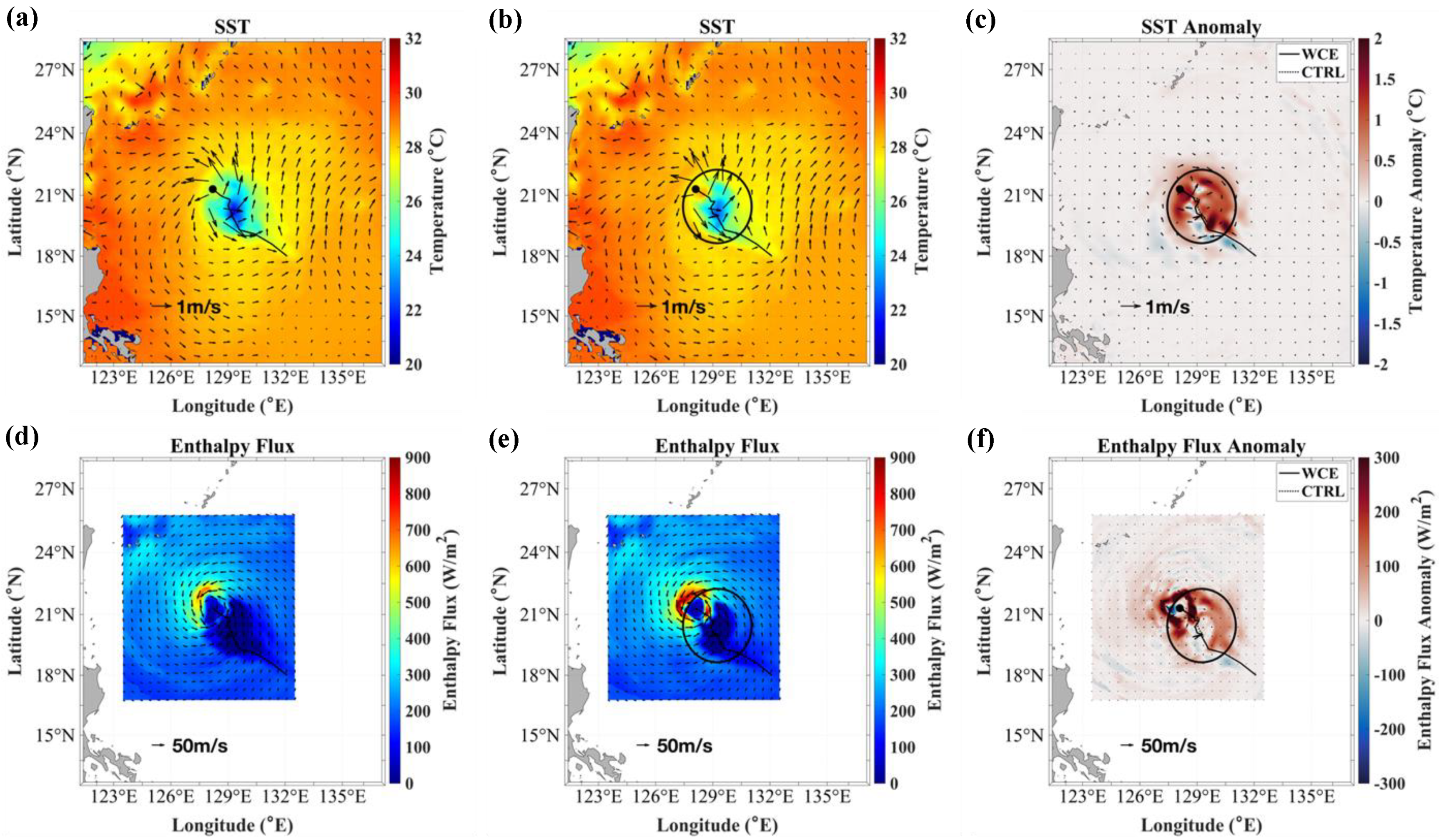
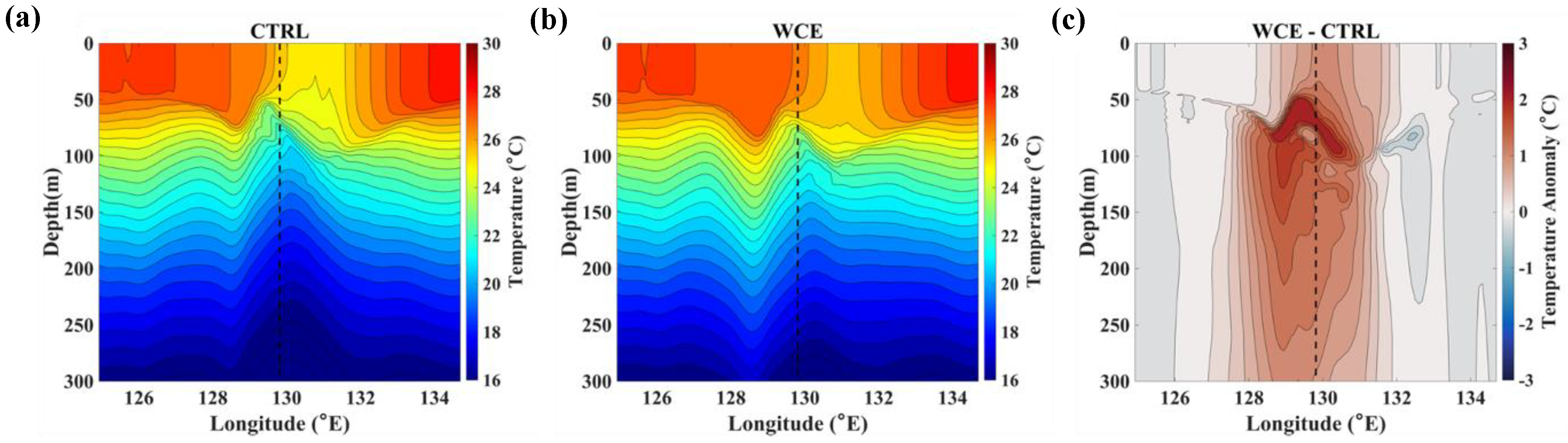
3.1. Ocean Response to TCs in Control Experiments

Before comparing the CTRL and WCE simulations, we first examine the ocean response and changes in TC intensity in the CTRL experiments. In the KONG-REY1 CTRL experiment initialized at 1800 UTC 30 September, the storm intensified during the first 24 h, as evidenced by the increased maximum wind speed and the decreased minimum central pressure (Figure 2). Figure 8a shows the pre-storm SST at 1800 UTC 30 September 2018. The plotted storm track indicates that for the first 24 h, the pre-storm SST exceeded 28.5 °C. However, this high temperature ahead of Kong-rey alone is not sufficient to explain the TC intensification, as it does not account for the SST cooling effect produced by the storm. A more accurate indicator of the available energy for the TC is the upper ocean heat content (OHC), also known as the tropical cyclone heat potential [8,48]. Figure 8b shows the pre-storm OHC calculated as

$$\mathrm{O}\mathrm{H}\mathrm{C}={\int }_0^{d26}\rho c_p\left[T\right(℃)-26]dz$$

(1)

where $d26$ is the depth of the 26 °C isotherms, $\rho$ is the seawater density, $c_p$ is a specific heat at constant pressure, $T$ is the ocean temperature, and $dz$ is the change in depth.

During the initial 24 h (from 1800 UTC 30 September to 1800 UTC 1 October), Kong-rey encountered high OHC exceeding 80 kJ/cm² (Figure 9c), which is greater than the threshold for TC intensification of 50 kJ/cm² [49]. The SST field at 1200 UTC 3 October indicates that the cooling caused by the storm did not exceed 1 °C during this period. This is consistent with the high OHC crossed by Kong-rey within the first 24 h, underscoring the favorable conditions for intensification.

The subsequent weakening of the storm, starting at 1800 UTC 2 October, is consistent with the lower OHC levels (20–40 kJ/cm²) encountered by Kong-rey (Figure 8b and Figure 9c). This weakening corresponds to the pre-existing SST cooling caused by the preceding TC Trami [50], which is evident at 19–22.5° N, 128–131° E in the GFS SST and, especially, OHC at 1800 UTC 30 September (Figure 8). However, the weakening phase is not accurately simulated compared to the best track data (Figure 2), which is consistent with the results of [31]. This suggests that other factors, such as the storm’s size, may have a more substantial impact on storm intensity than the pre-existing cooling.

In the JEBI1 CTRL experiment, initialized at 1200 UTC 30 August, the pre-storm SST along the track ranges from approximately 29 to 29.5 °C (Figure 10a). Similar to the Kong-rey case, the evolution of Jebi’s intensity can be explained by the magnitude and spatial distribution of the OHC. The storm gradually intensified over the first 24–30 h (Figure 2) while passing through an area with a high OHC of around 70 kJ/cm² (Figure 10b and Figure 9a). The subsequent decrease in the storm’s intensity, starting around 0000 UTC 1 September and continuing until landfall, is consistent with the lower OHC along the track, as seen in Figure 10b. Ref. [32] noted that their simulation failed to reproduce the observed maximum intensity of TC Jebi due to limitations in the atmospheric model’s horizontal resolution of 10 km and challenges in accurately representing the inner core structure. In our study, we used the HWRF model with the innermost domain having a horizontal resolution of 1.5 km, enabling us to simulate Jebi’s intensity evolution more accurately.

According to the JTWC best track data, Trami reached its peak intensity of 914 hPa at 1800 UTC 24 September and gradually weakened thereafter (Figure 2). This is consistent with our model simulation during Trami’s weakening phase. In the TRAMI1 CTRL experiment, initialized at 1800 UTC 23 September, the TC intensity significantly decreased between approximately 1800 UTC 24 September and 0000 UTC 27 September. This reduction was primarily due to Trami’s slow movement during this period, with a translation speed of 2–3 m/s, resulting in a large SST cooling. Figure 11 shows the spatial distributions of SST and zonal vertical cross-sections along 20.4° N at 0000 UTC 24 September (before the storm’s arrival) and 0000 UTC 27 September (during the storm). The maximum SST cooling reached about 6 °C just behind the storm center, which is in good agreement with the observations and model results from previous studies [31,33,34,35,36]. The slow propagation speed amplified the TC-driven ocean currents and vertical current shear, enhancing vertical mixing and the entrainment of colder water from the thermocline into the ocean surface layer. The relationship between the surface cooling rate and the storm’s translation speed has been extensively documented in early modeling studies [5]. The slow-moving Trami also caused strong upwelling near the storm center, as shown in the temperature cross-section in Figure 11d. The upwelling, driven by the divergence of the near-surface current induced by the TC’s cyclonic wind, brought deeper and cooler water closer to the sea surface, increasing the efficiency of vertical mixing and cooling of the SST. This effect often results in a rapid decrease in storm intensity [6].

Ref. [35] investigated the modulating effects of a pre-existing cold core eddy on upper ocean responses to Trami, revealing that the presence of the cold eddy enhances typhoon-induced sea surface cooling. However, Ref. [31] noted that the simulated intensity evolution of Trami, particularly during the rapid weakening phase, was not affected by including the cold core eddy in the initial oceanic conditions. Figure 9b shows the rapid decrease in OHC in the TRAMI1 CTRL simulation, falling below the threshold of intensification (50 kJ/cm², [49]) under the storm from 1200 UTC 25 September to 0000 UTC 27 September. This is consistent with the results of [31] (Figure 10a). Consequently, the intensity evolution of Trami in our simulations (Figure 2) matches the results shown in [31] (Figure 8b).

3.2. Ocean Response to TCs in WCE Experiments

In this section, we will discuss the TC simulations in which the ocean model is initialized with embedded WCEs. In all WCE experiments, the eddies were positioned along the TC track to assess their maximum impact on storm intensity. Figure 12, Figure 13 and Figure 14 compare the spatial distributions of the SST and enthalpy flux (latent and sensible heat flux) in the WCE and CTRL experiments for JEBI1, TRAMI1, and KONG-REY1, respectively. The locations of the WCEs are indicated by circles.

These figures were compiled at 0600 UTC 1 September in JEBI1 (Figure 12), 0600 UTC 27 September in TRAMI1 (Figure 13), and 1200 UTC 3 October in KONG-REY1 (Figure 14), representing the times the enthalpy flux differences between the WCE and CTRL experiments reached their maximum. The presence of WCEs has a significant impact on the SST response in all experiments. The SST anomalies calculated as WCE–CTRL (Figure 12c, Figure 13c and Figure 14c) show reduced SST cooling over WCEs, which resulted in increased enthalpy fluxes (Figure 12f, Figure 13f and Figure 14f). As expected, the magnitude of changes in the SST and enthalpy fluxes varies among the TC cases, depending on the specific storm characteristics and the pre-storm ocean conditions.

To examine the changes in the upper ocean thermal structure as the storm passes over the eddy, zonal vertical cross-sections through the storm center are compared in the CTRL and WCE experiments (Figure 15, Figure 16 and Figure 17). In the CTRL experiments, common features of the ocean response include the deepening of the mixed layer and a decrease in temperature. These changes in the upper ocean result from wind-induced vertical mixing, which is stronger to the right of the storm track due to the storm’s movement [5,6]. Another notable feature observed in the KONG-REY1 and TRAMI1 cases is the upwelling of cold thermocline water near the TC center, leading to enhanced cooling of the mixed layer. Trami produced the most significant upwelling due to its lowest translation speed among the three simulated TCs.

In the WCE experiments, mixed layer cooling was significantly reduced compared to the CTRL experiments, as indicated by the positive temperature differences in Figure 15c, Figure 16c and Figure 17c. The presence of deep warm water within the WCE, extending to depths of at least 300 m (Figure 5d), reduced the amount of cold water entrained into the mixed layer and substantially diminished the rate of vertical mixing. In the case of Trami, the strong upwelling generated near the storm center was capable of penetrating through the WCE warm layer (Figure 16b). Nevertheless, the mixed layer cooling was still considerably less than in the CTRL experiment.

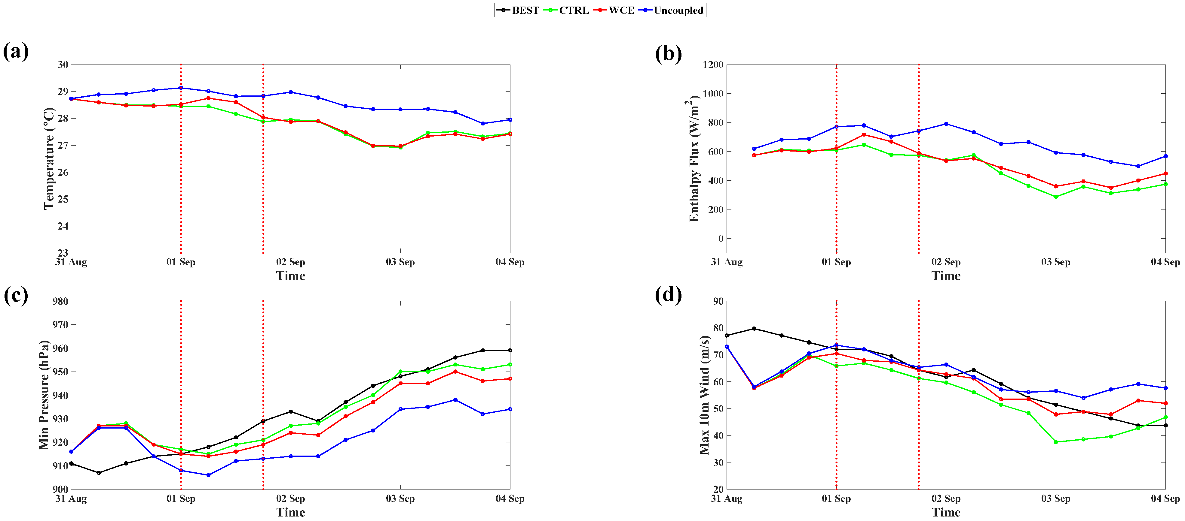
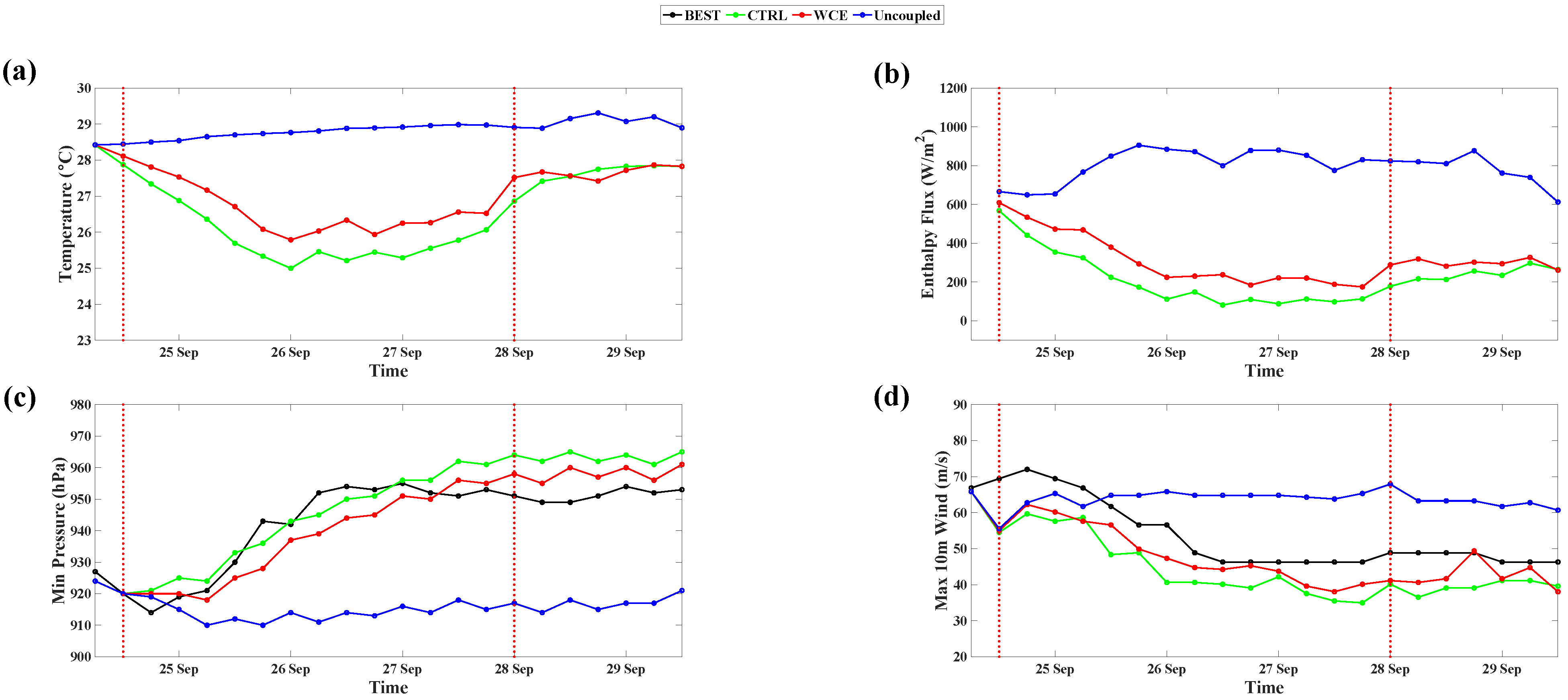
3.3. Impact of WCEs on TC Intensity

Figure 18, Figure 19, Figure 20, Figure 21, Figure 22 and Figure 23 show the minimum central pressures and maximum wind speeds in the uncoupled, coupled, and WCE experiments for all TC cases examined in this study: JEBI1, JEBI2, TRAMI1, TRAMI2, KONG-REY1, and KONG-REY2. As expected, the storm intensity in the uncoupled experiments is stronger in all TC cases than in the coupled experiments despite their following similar tracks (not shown). Note that [31] also found nearly identical track simulations in their coupled and uncoupled experiments. When the SST is fixed, it does not account for the SST cooling induced by storms, leading to an unlimited heat energy supply from the ocean for TC intensification. The largest differences in the TC intensity between the uncoupled and coupled experiments are found in Trami, which is the slowest-moving storm among the three simulated TCs. The slow movement of Trami allowed enough time to mix and cool the upper ocean beneath the storm and produced strong upwelling within the storm core area, as shown in Figure 16. This resulted in the largest differences in the averaged SST and enthalpy flux between the coupled and uncoupled experiments.

To better understand the impact of WCEs on TC intensity, the area-averaged SSTs, and enthalpy fluxes within a 100 km radius of the storm center are included in Figure 18, Figure 19, Figure 20, Figure 21, Figure 22 and Figure 23. Vertical dashed lines indicate the periods when the storms passed over the WCEs, determined by the time from when the storm’s radius of maximum wind enters and exits the WCE area. These lines only serve as reference points. It is important to note that the effects of the interaction between the TCs and the WCEs extended beyond these time periods, as evident in the figures. In the WCE experiments, the cooling of the ocean surface was inhibited over the eddies, as illustrated by the higher area-averaged SSTs compared to the control experiments in all three TCs (Figure 18a, Figure 19a, Figure 20a, Figure 21a, Figure 22a and Figure 23a). This inhibition is due to the presence of deep warm water with a high OHC within the WCE, as illustrated in Figure 11. This warm water acts as a barrier between the TC and the colder ocean water below [12].

Consequently, the reduced SST cooling resulted in higher enthalpy fluxes (Figure 18b, Figure 19b, Figure 20b, Figure 21b, Figure 22b and Figure 23b), transferring more heat energy from the ocean to the storms. The storm intensity increased during and after the eddy passage. The most significant increase in TC intensity is observed in Trami (Figure 20 and Figure 21), where the differences in the SST cooling and enthalpy fluxes over the eddy are the largest.

To quantitatively assess and compare the impacts of WCEs on SST, enthalpy fluxes, and TC intensity across all TC cases, we introduce a Maximum WCE Potential Index (MWPI). MWPI is defined as

$$\mathrm{M}\mathrm{W}\mathrm{P}\mathrm{I}=\frac{∆I_{WCE}}{∆I_{uncpl}}\times 100$$

(2)

where $∆I_{uncpl}$ represents the maximum difference between the uncoupled and CTRL experiments, and $∆I_{WCE}$ represents the maximum difference between the WCE and CTRL experiments. The maximum differences are calculated during the period starting when the storm enters the WCE until one day after it exits the WCE.

Table 2. Average maximum delta values and MWPI of two sets of experiments for each TC.

TC		SST (°C)	$\mathbf{EF}\left(\mathbf{W}/{\mathbf{m}}^2\right)$	$\mathbf{Pmin}\left(\mathbf{hPa}\right)$
	${∆I}_{WCE}$	0.43	100.51	6.00
JEBI	$∆I_{uncpl}$	1.27	256.97	12.50
	MWPI	33.9%	39.1%	48.0%
	${∆I}_{WCE}$	1.07	181.59	9.00
TRAMI	$∆I_{uncpl}$	3.36	735.99	43.50
	MWPI	31.8%	24.7%	20.7%
	${∆I}_{WCE}$	0.52	71.70	3.50
KONG-REY	$∆I_{uncpl}$	1.41	219.52	13.00
	MWPI	36.9%	32.7%	26.9%

presents the values of $∆I_{uncpl}$ and $∆I_{WCE}$ for the area-averaged SST, the area-averaged enthalpy flux (EF), and the minimum central pressure (Pmin), along with the calculated values of MWPI for TCs Jebi, Trami, and Kong-rey. Since we conducted two sets of experiments, 12 h apart, for each TC, the table displays the average values of $∆I_{uncpl}$, $∆I_{WCE}$, and MWPI between the two sets. Note that we did not calculate MWPI for the maximum wind speed due to its high-frequency fluctuations. The highest values of $∆I_{uncpl}$ and $∆I_{WCE}$ for SST and enthalpy flux are observed in TC Trami. In the CTRL experiment, the maximum SST cooling underneath the storm is $∆I_{uncpl}$ = 3.36 °C. However, in the WCE experiment, this cooling is reduced by $∆I_{WCE}$ = 1.07 °C. This reduction in SST cooling, combined with an increase in wind speed, results in a significant rise in enthalpy flux by $∆I_{WCE}$ = 181.59 W/m². Consequently, Trami experienced the largest increase in the minimum central pressure (9 hPa) among the simulated TCs.

Despite these significant changes, the MWPI value for Trami is only 24.7% for the enthalpy flux and 20.7% for Pmin. This is mainly due to the very strong SST cooling in this case, which led to the very large differences in enthalpy flux ($∆I_{uncpl}$ = 735.99 W/m²) and minimum pressure (43.5 hPa) between the CTRL and uncoupled experiments. The highest MWPI value for Pmin is found in Jebi (48%), followed by Kong-rey (26.9%). Overall, MWPI ranges from 31.8% to 36.9% for SST, 24.7 to 39.1% for enthalpy flux, and from 20.7 to 79.3% for minimum pressure across all experiments.

To investigate the influence of WCE size on storm intensification, we conducted additional sensitivity experiments using the JEBI1, TRAMI1, and KONG-REY1 cases, in which the WCE radii were set to 140, 200, and 300 km.

Table 3. Maximum delta values and MWPI in the WCE size sensitivity experiments for JEBI1, TRAMI1, and KONG-REY1.

Name		SST (°C)			$\mathbf{Pmin}\left(\mathbf{hPa}\right)$
		140 km	200 km	300 km	140 km	200 km	300 km
	${∆I}_{WCE}$	0.31	0.40	0.42	3	5	5
JEBI1	$∆I_{uncpl}$	1.14	1.14	1.14	16	16	16
	MWPI	27.2%	35.1%	36.8%	18.8%	31.3%	31.3%
	${∆I}_{WCE}$	0.77	0.80	0.97	12	13	14
TRAMI1	$∆I_{uncpl}$	3.75	3.75	3.75	44	44	44
	MWPI	20.5%	21.3%	25.9%	27.3%	29.5%	31.8%
	${∆I}_{WCE}$	0.50	0.66	0.73	2	3	9
KONG-REY1	$∆I_{uncpl}$	1.69	1.69	1.69	18	18	18
	MWPI	29.6%	39.1%	43.2%	11.1%	16.7%	50.0%

presents the calculated values of $∆I_{uncpl}$, $∆I_{WCE}$, and MWPI for SST and Pmin in these experiments. In most of these cases, TC interaction with a larger size WCE resulted in higher values of $∆I_{WCE}$ and MWPI. The differences in the impact of WCE on TC intensity are particularly significant between the small and large eddies in Jebi and Kong-rey, with MWPI for Pmin changing from 18.8% to 31.3% for Jebi, and 11.1% to 50% for Kong-rey. Trami’s MWPI for intensity exhibits less sensitivity to WCE size, varying from 27.3% to 31.8%, likely due to its slower translational speed.

4. Summary and Discussions

This numerical modeling study uses the HWRF atmospheric model coupled with the MPIPOM-TC ocean model to investigate the impact of warm core eddies (WCEs) on storm intensity in three Northwest Pacific tropical cyclones, Trami, Kong-rey, and Jebi, during 2018, representing slow-, medium, and fast-moving storms. To assess the impact of WCEs on TC intensity, three experiments are conducted for each storm: without WCE (control experiment), with fixed SST (uncoupled experiment), and with WCE included. In the WCE experiments, idealized WCEs are embedded into the three-dimensional MPIPOM-TC model fields.

The results of the control experiments demonstrate that SST distribution alone along the storm’s track cannot explain the simulated changes in storm intensity, as it does not account for storm-induced cooling. In all simulated TCs, the ocean heat content (OHC) along the track significantly influenced the storm intensity. For example, in Jebi and Kong-rey, the gradual intensification observed during the first day of simulations can be attributed to high OHC values along their respective tracks. These elevated OHC values, as observed in the North Equatorial Current (NEC) between 8° N and 17° N [51], reduce SST cooling, thus providing more heat energy for storm intensification. Despite the presence of high OHCs, the simulated rapid weakening of Trami is attributed to significant SST cooling caused by strong vertical mixing and upwelling underneath the storm due to its slow translation speed. In very slow-moving storms, upwelling reaches its peak in the storm’s eyewall region, where wind-induced mixing is the strongest.

This study uses uncoupled experiments with fixed SSTs as a reference for the TC maximum potential intensity, allowing for an unlimited energy supply for storm intensification. The largest TC intensity difference between the coupled and uncoupled simulations is found in Trami, mainly due to its slowest translation speed and largest SST cooling.

To investigate the impact of WCEs, experiments with and without an embedded WCE are conducted and compared. WCEs are placed at the same latitude in all experiments, with their centers positioned along the TC track to examine the maximum impact on storm intensity. To quantify the WCE effect, area-averaged values of SST and enthalpy flux within a 100 km radius of the storm center are calculated. The results indicate that in all TCs, regardless of the storm translation speed, the presence of WCEs reduces the storm-induced upper ocean cooling and increases enthalpy flux. The most significant impact of WCEs on reducing SST cooling is found in Trami, which is the slowest-moving TC. Although strong upwelling generated by Trami is capable of penetrating through the WCE warm layer, the mixed layer cooling is still considerably less than in the CTRL experiment. In all TC experiments, more heat energy is supplied to the storms during their passage over WCEs, leading to intensification as indicated by the decrease in central pressure and the increase in maximum wind speed.

To quantitatively assess the impact of WCEs on ocean response and TC intensity across all the simulated TC cases, a Maximum WCE Potential Index (MWPI) is introduced. For a WCE with a 200 km radius, MWPI ranges from 31.8% to 36.9% in reducing the SST cooling and from 24.7% to 39.1% in increasing enthalpy fluxes. MWPI varies from 26.9% to 48% in increasing TC intensity, measured by the minimum central pressure (Pmin). These results indicate that although all simulated TCs interact with practically the same WCE, MWPI can vary significantly due to the differences in storm intensity and translation speed. Sensitivity experiments with small (140 km radius) and large (300 km radius) WCEs reveal higher MWPI values when TCs interact with larger WCEs. MWPI differences in Pmin between the small and large eddies range from 18.8% to 31.3% for Jebi, 27.3% to 31.8% for Trami, and 11.1% to 50% for Kong-rey. The lower sensitivity of the MWPI values to WCE size in Trami is likely due to its slower translational speed.

In our study, we assimilated real-time GFS SSTs into the initial temperature fields. Although the GFS SST has a relatively coarse resolution, we successfully captured the intensity evolution of TCs, similar to previous studies that utilized higher-resolution HYCOM SST data. However, we recognize the importance of accurately representing SST conditions to fully capture the dynamics of TCs and their interactions with WCEs.

While this study models real TCs, using artificial WCEs introduces certain limitations in making accurate assessments of storm intensity changes. To improve our understanding of the role of WCEs in TCs and quantify their impacts, it is imperative to undertake more realistic modeling studies in the future, using fully coupled TC–ocean models in conjunction with field observations. Such studies are important for improving TC intensity prediction, which remains a challenging problem.

References

1. Emanuel, K.A. An air-sea interaction theory for tropical cyclones. Part I: Steady-state maintenance. J. Atmos. Sci. 1986, 43, 585–605. [Google Scholar] [CrossRef]
2. Cione, J.J.; Uhlhorn, E.W. Sea surface temperature variability in hurricanes: Implications with respect to intensity change. Mon. Weather Rev. 2003, 131, 1783–1796. [Google Scholar] [CrossRef]
3. Bao, J.W.; Fairall, C.W.; Michelson, S.A.; Bianco, L. Parameterizations of sea-spray impact on the air–sea momentum and heat fluxes. Mon. Weather Rev. 2011, 139, 3781–3797. [Google Scholar] [CrossRef]
4. Kowaleski, A.M.; Evans, J.L. Thermodynamic observations and flux calculations of the tropical cyclone surface layer within the context of potential intensity. Weather Forecast. 2015, 30, 1303–1320. [Google Scholar] [CrossRef]
5. Price, J.F. Upper ocean response to a hurricane. J. Phys. Oceanogr. 1981, 11, 153–175. [Google Scholar] [CrossRef]
6. Ginis, I. Tropical cyclone-ocean interactions. Adv. Fluid Mech. Ser. 2002, 33, 83–114. [Google Scholar]
7. Bender, M.A.; Ginis, I. Real-case simulations of hurricane–ocean interaction using a high-resolution coupled model: Effects on hurricane intensity. Mon. Weather Rev. 2000, 128, 917–946. [Google Scholar] [CrossRef]
8. Shay, L.K.; Goni, G.J.; Black, P.G. Effects of a warm oceanic feature on hurricane Opal. Mon. Weather Rev. 2000, 128, 1366–1383. [Google Scholar] [CrossRef]
9. Schade, L.R.; Emanuel, K.A. The ocean’s effect on the intensity of tropical cyclones: Results from a simple coupled atmosphere–ocean model. J. Atmos. Sci. 1999, 56, 642–651. [Google Scholar] [CrossRef]
10. Chan, J.C.L.; Duan, Y.; Shay, L.K. Tropical cyclone intensity change from a simple ocean–atmosphere coupled model. J. Atmos. Sci. 2001, 58, 154–172. [Google Scholar] [CrossRef]
11. Jaimes, B.; Shay, L.K.; Uhlhorn, E.W. Enthalpy and momentum fluxes during hurricane Earl relative to underlying ocean features. Mon. Weather Rev. 2015, 143, 111–131. [Google Scholar] [CrossRef]
12. Lin, I.-I.; Wu, C.-C.; Emanuel, K.A.; Lee, I.-H.; Wu, C.-R.; Pun, I.-F. The interaction of supertyphoon Maemi (2003) with a warm ocean eddy. Mon. Weather Rev. 2005, 133, 2635–2649. [Google Scholar] [CrossRef]
13. Wang, G.; Zhao, B.; Qiao, F.; Zhao, C. Rapid intensification of super typhoon Haiyan: The important role of a warm-core ocean eddy. Ocean Dyn. 2018, 68, 1649–1661. [Google Scholar] [CrossRef]
14. Hong, X.; Chang, S.W.; Raman, S.; Shay, L.K.; Hodur, R. The interaction between hurricane Opal (1995) and a warm core ring in the Gulf of Mexico. Mon. Weather Rev. 2000, 128, 1347–1365. [Google Scholar] [CrossRef]
15. Emanuel, K.; DesAutels, C.; Holloway, C.; Korty, R. Environmental control of tropical cyclone intensity. J. Atmos. Sci. 2004, 61, 843–858. [Google Scholar] [CrossRef]
16. Wu, C.-C.; Lee, C.-Y.; Lin, I.-I. The effect of the ocean eddy on tropical cyclone intensity. J. Atmos. Sci. 2007, 64, 3562–3578. [Google Scholar] [CrossRef]
17. McTaggart-Cowan, R.; Bosart, L.F.; Gyakum, J.R.; Atallah, E.H. Hurricane Katrina (2005). Part I: Complex life cycle of an intense tropical cyclone. Mon. Weather Rev. 2007, 135, 3905–3926. [Google Scholar] [CrossRef]
18. Vianna, M.L.; Menezes, V.V.; Pezza, A.B.; Simmonds, I. Interactions between hurricane Catarina (2004) and warm core rings in the South Atlantic ocean. J. Geophys. Res. 2010, 115, C07002. [Google Scholar] [CrossRef]
19. Yablonsky, R.M.; Ginis, I. Impact of a warm ocean eddy’s circulation on hurricane-induced sea surface cooling with implications for hurricane intensity. Mon. Weather Rev. 2012, 141, 997–1021. [Google Scholar] [CrossRef]
20. Jaimes, B.; Shay, L.K. Enhanced wind-driven downwelling flow in warm oceanic eddy features during the intensification of tropical cyclone Isaac (2012): Observations and theory. J. Phys. Oceanogr. 2015, 45, 1667–1689. [Google Scholar] [CrossRef]
21. Jaimes, B.; Shay, L.K.; Brewster, J.K. Observed air-sea interactions in tropical cyclone Isaac over Loop Current mesoscale eddy features. Dyn. Atmos. Ocean. 2016, 76, 306–324. [Google Scholar] [CrossRef]
22. Emanuel, K. Increasing destructiveness of tropical cyclones over the past 30 years. Nature 2005, 436, 686–688. [Google Scholar] [CrossRef] [PubMed]
23. Peduzzi, P.; Chatenoux, B.; Dao, H.; De Bono, A.; Herold, C.; Kossin, J.; Mouton, F.; Nordbeck, O. Global trends in tropical cyclone risk. Nat. Clim. Chang. 2012, 2, 289–294. [Google Scholar] [CrossRef]
24. Lin, I.-I.; Black, P.; Price, J.F.; Yang, C.-Y.; Chen, S.S.; Lien, C.-C.; Harr, P.; Chi, N.-H.; Wu, C.-C.; D’Asaro, E.A. An ocean coupling potential intensity index for tropical cyclones. Geophys. Res. Lett. 2013, 40, 1878–1882. [Google Scholar] [CrossRef]
25. Qiu, B. Seasonal eddy field modulation of the North Pacific subtropical countercurrent: TOPEX/Poseidon Observations and Theory. J. Phys. Oceanogr. 1999, 29, 2471–2486. [Google Scholar] [CrossRef]
26. Roemmich, D.; Gilson, J. Eddy transport of heat and thermocline waters in the North Pacific: A key to interannual/decadal climate variability? J. Phys. Oceanogr. 2001, 31, 675–687. [Google Scholar] [CrossRef]
27. Hwang, C.; Wu, C.-R.; Kao, R. TOPEX/Poseidon observations of mesoscale eddies over the subtropical countercurrent: Kinematic characteristics of an anticyclonic eddy and a cyclonic eddy. J. Geophys. Res. Ocean. 2004, 109. [Google Scholar] [CrossRef]
28. Yablonsky, R.M.; Ginis, I. Limitation of one-dimensional ocean models for coupled hurricane–ocean model forecasts. Mon. Weather Rev. 2009, 137, 4410–4419. [Google Scholar] [CrossRef]
29. Ma, Z.; Fei, J.; Liu, L.; Huang, X.; Li, Y. An investigation of the influences of mesoscale ocean eddies on tropical cyclone intensities. Mon. Weather Rev. 2017, 145, 1181–1201. [Google Scholar] [CrossRef]
30. Sun, J.; Wang, G.; Xiong, X.; Hui, Z.; Hu, X.; Ling, Z.; Yu, L.; Yang, G.; Guo, Y.; Ju, X.; et al. Impact of warm mesoscale eddy on tropical cyclone intensity. Acta Oceanol. Sin. 2020, 39, 1–13. [Google Scholar] [CrossRef]
31. Wada, A. Roles of oceanic mesoscale eddy in rapid weakening of typhoons Trami and Kong-Rey in 2018 simulated with a 2-km-mesh atmosphere-wave-ocean coupled model. J. Meteorol. Soc. Jpn. 2021, 99, 1453–1482. [Google Scholar] [CrossRef]
32. Kawakami, Y.; Nakano, H.; Urakawa, L.S.; Toyoda, T.; Sakamoto, K.; Yoshimura, H.; Shindo, E.; Yamanaka, G. Interactions between ocean and successive typhoons in the Kuroshio region in 2018 in atmosphere–ocean coupled model simulations. J. Geophys. Res. Ocean. 2022, 127, e2021JC018203. [Google Scholar] [CrossRef]
33. Chang, K.F.; Wu, C.C.; Ito, K. On the rapid weakening of typhoon Trami (2018): Strong sea surface temperature cooling associated with slow translation speed. Mon. Weather Rev. 2023, 151, 227–251. [Google Scholar] [CrossRef]
34. Li, X.; Cheng, X.; Fei, J.; Huang, X.; Ding, J. The modulation effect of sea surface cooling on the eyewall replacement cycle in typhoon Trami (2018). Mon. Weather Rev. 2022, 150, 1417–1436. [Google Scholar] [CrossRef]
35. Li, X.; Cheng, X.; Fei, J.; Huang, X. A numerical study on the role of mesoscale cold-core eddies in modulating the upper-ocean responses to typhoon Trami (2018). J. Phys. Oceanogr. 2022, 52, 3101–3122. [Google Scholar] [CrossRef]
36. Hirano, S.; Ito, K.; Yamada, H.; Tsujino, S.; Tsuboki, K.; Wu, C.C. Deep eye clouds in tropical cyclone Trami (2018) during T-PARCII dropsonde observations. J. Atmos. Sci. 2022, 79, 683–703. [Google Scholar] [CrossRef]
37. Tallapragada, V.; Bernardet, L.; Biswas, M.K.; Gopalakrishnan, S.; Kwon, Y.; Liu, Q.; Marchok, T.; Sheinin, D.; Tong, M.; Trahan, S.; et al. Hurricane Weather Research and Forecasting (HWRF) model: 2013 scientific documentation. HWRF Dev. Testbed Cent. Tech. Rep. 2014, 99, 1–13. Available online: http://www.dtcenter.org/HurrWRF/users/docs/ (accessed on 3 February 2024).
38. Biswas, M.K.; Carson, L.; Newman, K.; Bernardet, L.; Kalina, E.; Grell, E.; Frimel, J. Community HWRF Users Guide v3.9a. 2018. Available online: https://repository.library.noaa.gov/view/noaa/16281 (accessed on 3 February 2024).
39. Yablonsky, R.M.; Ginis, I.; Thomas, B.; Tallapragada, V.; Sheinin, D.; Bernardet, L. Description and analysis of the ocean component of NOAA’s operational Hurricane Weather Research and Forecasting Model (HWRF). J. Atmos. Ocean. Technol. 2015, 32, 144–163. [Google Scholar] [CrossRef]
40. Yablonsky, R.M.; Ginis, I.; Thomas, B. Ocean modeling with flexible initialization for improved coupled tropical cyclone-ocean model prediction. Environ. Model. Softw. 2015, 67, 26–30. [Google Scholar] [CrossRef]
41. Mellor, G.L.; Yamada, T. Development of a turbulence closure model for geophysical fluid problems. Rev. Geophys. 1982, 20, 851. [Google Scholar] [CrossRef]
42. Carnes, M.R. Description and Evaluation of GDEM-V 3.0; Naval Research Laboratory: Washington, DC, USA, 2009; pp. 1–24. [Google Scholar]
43. Reynolds, R.W.; Smith, T.M. Improved global sea surface temperature analyses using optimum interpolation. J. Clim. 1994, 7, 929–948. [Google Scholar] [CrossRef]
44. Yablonsky, R.M.; Ginis, I. Improving the ocean initialization of coupled hurricane–ocean models using feature-based data assimilation. Mon. Weather Rev. 2008, 136, 2592–2607. [Google Scholar] [CrossRef]
45. Trahan, S.; Sparling, L. An analysis of NCEP tropical cyclone vitals and potential effects on forecasting models. Weather Forecast. 2012, 27, 744–756. [Google Scholar] [CrossRef]
46. Cheng, Y.H.; Ho, C.R.; Zheng, Q.; Kuo, N.J. Statistical characteristics of mesoscale eddies in the North Pacific derived from satellite altimetry. Remote Sens. 2014, 6, 5164–5183. [Google Scholar] [CrossRef]
47. Liu, Y.; Dong, C.; Guan, Y.; Chen, D.; McWilliams, J.; Nencioli, F. Eddy analysis in the subtropical zonal band of the North Pacific ocean. Deep Sea Res. Part I Oceanogr. Res. Pap. 2012, 68, 54–67. [Google Scholar] [CrossRef]
48. Wada, A.; Usui, N. Importance of tropical cyclone heat potential for tropical cyclone intensity and intensification in the Western North Pacific. J. Oceanogr. 2007, 63, 427–447. [Google Scholar] [CrossRef]
49. Wada, A. Verification of tropical cyclone heat potential for tropical cyclone intensity forecasting in the Western North Pacific. J. Oceanogr. 2015, 71, 373–387. [Google Scholar] [CrossRef]
50. Song, D.; Xiang, L.; Guo, L.; Li, B. Estimating typhoon-induced sea surface cooling based upon satellite observations. Water 2020, 12, 3060. [Google Scholar] [CrossRef]
51. Kang, S.K.; Kim, S.-H.; Lin, I.-I.; Park, Y.-H.; Choi, Y.; Ginis, I.; Cione, J.; Shin, J.Y.; Kim, E.J.; Kim, K.O.; et al. The North Equatorial Current and rapid intensification of super typhoons. Nat. Commun. 2024, 15, 1742. [Google Scholar] [CrossRef]
Figure 1. The HWRF coupled model domains. The region with SST is the outer HWRF domain. The blue box is the Northwest Pacific MPIPOM-TC domain. The black solid boxes inside show the sizes of the intermediate and innermost movable HWRF domains.
Atmosphere 15 00445 g001
Figure 2. Upper panels: tracks of JTWC BEST and control experiments for TCs Jebi, Trami, and Kong-rey. Circles indicate the storm center every 6 h. Middle panels: minimum central pressure (hPa) and Lower panels: 10 m maximum wind speed (m/s) in JTWC BEST and control experiments every 6 h as a function of time.
Atmosphere 15 00445 g002
Figure 3. (a) AVISO sea surface height anomaly (m) on 21 September 2017. The eddy edges are enclosed by black lines. (b) Temperature (°C) profiles in the background (black line) based on GDEM climatology and the center of WCE (red line) based on the WCE observed during Typhoon Maemi.
Atmosphere 15 00445 g003
Figure 4. (a) Spatial distribution of temperature (°C) at 75 m in the idealized WCE. (b) Zonal vertical cross-section through the center of WCE. Vertical dashed line indicates the WCE center.
Atmosphere 15 00445 g004
Figure 5. (a) Spatial distribution of temperature (°C) at 75 m in GDEM climatology, and (c) zonal vertical cross-section at 20.4° N along the dashed line in (a). (b,d) after WCE with 200 km radius assimilation into GDEM climatology for TC Kong-rey experiment initialized at 1800 UTC 30 September (KONG-REY1). BEST track and center positions of Kong-rey every 6 h are overlaid in (b). Vertical dashed line in (d) indicates the center of WCE.
Atmosphere 15 00445 g005
Figure 6. Same as Figure 5, but for (a,c) WCE with 140 km and (b,d) WCE with 300 km radius.
Atmosphere 15 00445 g006
Figure 7. Spatial distribution of sea surface height anomaly (m) at 1800 UTC 30 September in the KONG-REY1 experiments (a) WCE (140), (b) WCE (200), and (c) WCE (300). SSHA is calculated from the model output (WCE–CTRL). Simulated track and center positions of Kong-rey every 6 h are overlaid.
Atmosphere 15 00445 g007
Figure 8. Spatial distribution of (a) SST (°C) and (b) OHC (kJ/cm2) with ocean currents for KONG-REY1 CTRL experiment at 1800 UTC 30 September. The storm track is shown by the black line.
Atmosphere 15 00445 g008
Figure 9. Time series of area-averaged OHC (kJ/cm2) for (a) JEBI1, (b) TRAMI1, and (c) KONG-REY1. OHC is calculated within 100 km radius. Vertical red dashed lines indicate the time period when the storm passed over WCE.
Atmosphere 15 00445 g009
Figure 10. Same as Figure 8, but for JEBI1 CTRL experiment at 1200 UTC 30 August.
Atmosphere 15 00445 g010
Figure 11. Spatial distribution of SST (°C) with ocean currents for TRAMI1 CTRL experiment (a) at 0000 UTC 24 September and (c) at 0000 UTC 27 September. Zonal vertical cross sections at 20.4° N (b) at 0000 UTC 24 September and (d) at 0000 UTC 27 September.
Atmosphere 15 00445 g011
Figure 12. Spatial distribution of SST (°C) and enthalpy flux (W/m2) in (a,d) CTRL, (b,e) WCE experiments, and (c,f) anomaly (WCE–CTRL) for JEBI1 at 0600 UTC 1 September. The black circle indicates the location and approximate size of WCE, and the black dot indicates the storm center. The lines indicate the storm tracks in WCE and CTRL experiments.
Atmosphere 15 00445 g012
Figure 13. Same as Figure 12, but for TRAMI1 at 0600 UTC 27 September.
Atmosphere 15 00445 g013
Figure 14. Same as Figure 12, but for KONG-REY1 at 1200 UTC 3 October.
Atmosphere 15 00445 g014
Figure 15. Zonal vertical cross section of temperature (°C) at the center of WCE in (a) CTRL, (b) WCE, and (c) anomaly (WCE–CTRL) for JEBI1 at 0600 UTC 1 September. Vertical dashed line indicates the center of WCE.
Atmosphere 15 00445 g015
Figure 16. Same as Figure 15, but for TRAMI1 at 0600 UTC 27 September.
Atmosphere 15 00445 g016
Figure 17. Same as Figure 15, but for KONG-REY1 at 1200 UTC 3 October.
Atmosphere 15 00445 g017
Figure 18. Time series of area-averaged (a) SST (°C), (b) enthalpy flux (W/m2) within 100 km radius, (c) minimum central pressure (hPa), and (d) 10 m maximum wind speed (m/s) for JEBI1. Vertical red dashed lines indicate the time period when the storm passed over WCE.
Atmosphere 15 00445 g018
Figure 19. Same as Figure 18, but for JEBI2.
Atmosphere 15 00445 g019
Figure 20. Same as Figure 18, but for TRAMI1.
Atmosphere 15 00445 g020
Figure 21. Same as Figure 18, but for TRAMI2.
Atmosphere 15 00445 g021
Figure 22. Same as Figure 18, but for KONG-REY1.
Atmosphere 15 00445 g022
Figure 23. Same as Figure 18, but for KONG-REY2.
Atmosphere 15 00445 g023