1. Introduction
Atmospheric aerosol has a direct impact on the atmospheric radiative balance and global climate cycles. It also plays an indirect role in determining the microphysical properties of clouds, which affects physical processes in clouds and the formation of atmospheric precipitation. Aerosol is one of the crucial components in the hydrological cycle. We only refer to the interaction of aerosols with water, which is a significant aspect of aerosol physics. Aerosol particles serve as the nucleus of cloud particle formation, and increased concentrations of aerosol particles modify the microphysical, optical, and radiative properties of clouds. On the other hand, clouds and precipitation trap polluting aerosols, removing them from the atmosphere, a process known as wet aerosol removal, which is important in air pollution studies [
1,
2].
Despite the importance of aerosols, their influence on global atmospheric processes has not been fully investigated. Describing their impact on climate is always a challenge. Aerosol dynamics are defined by various and complex mathematical models [
3,
4]. This statement can be supported by several arguments:
- (i)
The physical-chemical properties of aerosols;
- (ii)
The interaction processes of aerosols with water present in the three states of aggregation in the atmosphere;
- (iii)
The interaction processes of solar radiation with aerosols.
In such a framework, since theoretical mathematical models describing atmospheric dynamics involve the use of nonlinear differential equations, analytical solutions are more difficult to obtain (note that analytical solutions are usually correlated, either special symmetries or adequate boundary conditions [
3]). Because of the nonlinearities mentioned above, computational methods are usually preferred.
Computational models are commonly used, either in integer or fractional manifold space (the manifolds in which one operates with
—order differentials are defined as integer manifolds, while the manifolds in which fractional differentials are operated are called fractional manifold) [
5,
6]. The description of atmospheric dynamics can be enhanced by using Scale Relativity Theory [
7,
8], either for mono-fractal or multifractal atmospheric dynamics. In both cases, the dynamics of the structural units of any type of atmosphere, which is considered a complex system, are described by continuous and non-differentiable curves (fractal curves/multifractal curves). More precisely, by using motion curves with a single fractal dimension, only mono-fractal atmospheric dynamics can be specified [
9], while by using motion curves that can have several fractal dimensions simultaneously, multifractal atmospheric dynamics can be specified [
10,
11]. This procedure has resulted in the following:
- (i)
A β model for the generation and analysis of atmospheric turbulence [
12];
- (ii)
A computational method for the determination of the planetary boundary layer and its properties [
13];
- (iii)
The removal of atmospheric turbulence through laminar channels [
14].
Rosu et al. [
12] proposed a multifractal model to understand the dynamics of the turbulent atmosphere by reducing it to the standard β model. The authors suggest that the turbulent atmosphere can be considered a complex system, with its structural units supporting dynamics on continuous but non-differentiable multifractal curves. The authors implement the multifractality approach through the theoretical framework of scale relativity theory with arbitrary and constant fractal dimension, using non-differentiable functions. They argue that the atmosphere is a multifractal due to the continuous and non-differentiable curves of atmospheric particles’ trajectories. The equations that underpin atmospheric dynamics are expressed using a scale covariant derivative operator to describe the behaviour of these atmospheric entities [
8,
15,
16].
Ice clouds, also known as cirrus clouds, are important for Earth’s climate system and atmospheric processes. They are high-altitude clouds made up of ice crystals and are typically found in the upper troposphere and lower stratosphere [
17,
18].
Accurately modelling ice clouds is crucial in contemporary atmospheric science due to their significant influence on global climate, weather patterns, and radiative forcing, and their connection to various environmental and societal issues [
19,
20]. Ice clouds have a profound impact on the Earth’s energy balance by affecting both incoming solar radiation and outgoing terrestrial radiation. They possess unique radiative properties that regulate the Earth’s temperature. Ice crystals reflect incoming sunlight, but they also trap heat emitted by the Earth, contributing to the greenhouse effect [
21,
22,
23]. Accurate modelling of ice clouds is essential for assessing their role in global warming, climate change, weather forecasting, and air traffic and aviation.
This paper presents an alternative approach to ice cloud dynamics by implementing the previously discussed mechanisms of atmospheric laminar channels [
14]. Rosu et al. [
12] recently presented a mathematical model that describes the motion of atmospheric entities, considering both differential and non-differential scale resolutions. The model is based on a set of differential equations for the velocity fields, which reflect the interdependent complex mechanisms involved in the motion of atmospheric entities. The concept of multifractalization by Markov-type stochastic processes was introduced by the authors [
24]. This involves specific coefficients that are associated with the transitions from multifractal to non-multifractal states. In atmospheric dynamics, two distinct patterns emerge based on stochastic fractalization/multifractalization: monofractal patterns exhibit homogeneous behaviour with a single fractal dimension and consistent scaling across time intervals, and multifractal patterns display non-homogeneous behaviour with multiple fractal dimensions, allowing for the identification of universal patterns in atmospheric dynamics despite apparent differences [
8,
9,
25].
This paper investigates non-linear behaviours in atmospheric aerosol dynamics at the transition between turbulent and laminar flows using the Scale Relativity Theory. The article is structured as follows: The ‘Theoretical Model’ section presents a mathematical model that defines, by means of differentiable and nondifferentiable spatial-temporal coordinates, both the differentiable and non-differentiable velocities, and specific constants related to transitions from laminar to turbulence in the atmospheric dynamics. In such context, the singularity spectrum characterizes atmospheric dynamics, emphasizing nature of the atmosphere as a complex system. This section presents an analysis of how differential equations can be used to model the behaviour of atmospheric aerosols at different scales, incorporating diffusion processes and deposition mechanisms within turbulent and laminar dynamics. It also discusses the solution of diffusion equations for initial one-dimensional distributions in unbounded media using Fourier integrals. The ‘Results’ section presents a study that analysed atmospheric dynamics using data on radar reflectivity factor and ceilometer. The theoretical approach was correlated using experimental data from ceilometer and radar reflectivity factor data, which identified laminar channels at specific altitudes and scales. The analysis revealed patterns of ascending and descending laminar channels at different altitudes, providing insights into atmospheric stability and cloud formations. The final section contains the discussions and conclusions.
2. Theoretical Model
It is acknowledged, in accordance with references [
12,
13,
14], that the atmosphere can be represented as a fractal/multi-fractal mathematical object, both structurally and functionally. The dynamics of this object, as described by the Multifractal Theory of Motion [
10], is represented by continuous and non-differentiable curves (multifractal curves), which implies the functionality of the scale covariant derivative.
where we used the following notations:
In relations (1) and (2),
represents the spatial coordinates, described by continuous and nondifferentiable mathematical functions that depend on scale resolution. The temporal coordinate,
t, is described by continuous and differentiable mathematical functions that are independent of scale resolution.
represents the differentiable velocity (i.e., the velocity at differential scale resolution), while
represents the nondifferentiable velocity (i.e., the velocity at nondifferentiable scale resolution).
and
are specific constants of the differentiable-nondifferentiable scale transition associated with the forward and backward atmospheric dynamics, respectively. The singularity spectrum of order
, denoted by
, is determined by
, where
is the fractal dimension of the motion curves of the structural units of any atmosphere. It is important to note that the atmosphere is always assimilated to a complex system [
8,
11,
12,
13,
14].
In this context, using the singularity spectrum of order to describe atmospheric dynamics has clear advantages:
The dynamics of the structural units of the atmosphere may exhibit a dominant fractal dimension, which could aid in identifying a global atmospheric pattern that is compatible with a certain global atmospheric structurality and functionality.
The dynamics of the structural units of the atmosphere may contain a “set” of fractal dimensions, which could aid in identifying zonal atmospheric patterns that are compatible with specific local atmospheric structures and functions.
Through the -order singularity spectrum, one can identify universality classes in the field of atmospheric dynamics, even when the attractors associated with these dynamics have different aspects.
The explicit form of the tensor
, i.e., that associated with the non-multifractal scale transition, is dictated by multifractalization through stochasticity. The most common method of fractalization is through stochastic processes [
9,
10]. In this context, it is important to clarify that the stochastic or chaotic processes used in the study of atmospheric dynamics can be categorized into two types. The first type includes homogeneous atmospheric dynamics, which are characterized by a single global fractal dimension and exhibit the same scaling properties in any time interval (such as fractional Brownian processes). The second category comprises atmospheric dynamics that can be described using multiple fractal dimensions and quantify only local singularities, known as multifractal processes.
Therefore, we can distinguish following types of atmospheric dynamics:
- i.
Multifractal atmospheric dynamics via Markov stochasticity imposed by the following constraints [
7,
24]:
where
is a diffusion-type coefficient associated with the multifractal-non-multifractal scale transition and
is the Kronecker pseudotensor. In such an alternative:
so that Equation (1)becomes as follows:
- ii.
Multifractal atmospheric dynamics by non-Markov stochasticity imposed by the following constraints [
12,
13]:
where
and
are diffusion-type coefficients associated with the multifractal-non-multifractal scale transition. In such an alternative:
so that Equation (1) becomes the following:
Assuming now the functionality of the principle of scale covariance, according to which the laws of atmospheric physics remain invariant with respect to both spatial and temporal transformations and scale transformations, different conservation laws can be constructed.
For example, if one applies the complex operator (8) to the density of states
, then the conservation law takes the following form:
or yet, explained on resolution scales as follows:
at differential scale resolutions, i.e., as follows:
at non-differential scale resolutions. Next if we denote with the following:
the velocity associated with the multifractal-non-multifractal scale transition, by adding relations (10) and (11), the conservation law of the density of states associated with the multifractal-non-multifractal scale transition is obtained as follows:
In the following, we present the consequences of such a differential equation in modelling atmospheric dynamics. For this purpose, let us consider the differential Equation (13) in the one-dimensional case and subject to the following constraint:
This becomes the following:
where we made the notation as follows:
where
D depends on the aerosols (geometrical and physical properties), atmosphere, and scale resolution scale properties.
The above model can describe, for example, at various scale resolutions, nonlinear behaviours of atmospheric aerosols that obey simultaneously diffusion and deposition processes through transitions from turbulence to laminar dynamics (diffusion and deposition processes are discussed in their classical sense, with no reference to optical processes). From this perspective, the turbulence–laminar transition will work as multifractal–nonmultifractal scale transition where V denotes the deposition rate associated with such transition.
By making the variable change as follows:
which implies the following:
the differential Equation (15) becomes as follows:
From the initial conditions and the boundary one as follows:
the boundary conditions corresponding to
n are obtained, i.e., as follows:
This problem can be reduced to one without boundary conditions by extending the solution to include the region
, where
n assumes an initial distribution that simulates the boundary condition for
at any time
. At the same time one can choose the following:
so that for any extended region, the initial condition will be as follows:
The problem is how to solve the diffusion equation for an initially specified dimensional distribution in an unbounded medium. This can be solved by developing the solution as a Fourier integral:
After substituting the differential Equation (19) we obtain the following:
with the solution as follows:
where
was obtained by substituting the initial distribution
n into Equation (25). Therefore, Equation (24)can be expressed as an integral over the entire initial distribution as follows:
Once the integral above is resolved with respect to
k, solving it for
n becomes straightforward, leading to the following:
The solution can be completed by substituting Equation (23) into Equation (29) and calculating the integral. The result for
is given by the following equation:
where
is the Laplace function given by the following:
values of this function being tabulated.
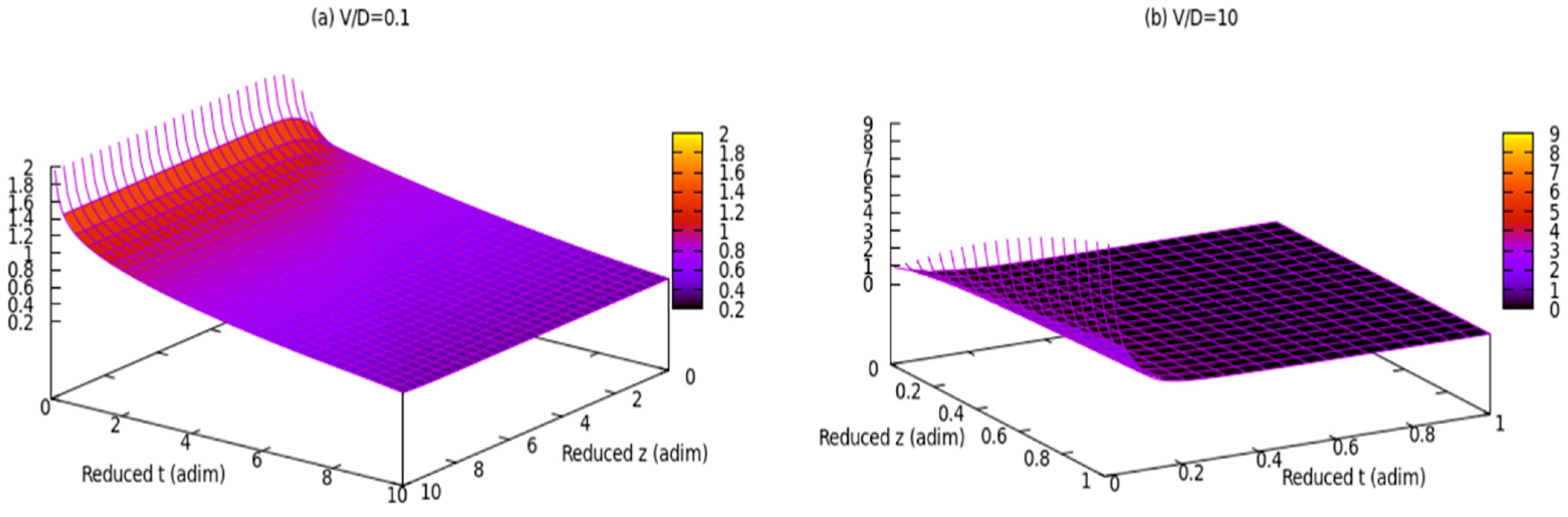
In
Figure 1, we illustrate the variations in dimensionless coordinates (used here as ‘
adim’), namely reduced
z(
adim) and reduced
t(
adim), with respect to density dependencies. It is evident that, at a dimensionless rate of
,
experiences an initial increase with reduced
z(
adim) for small values of reduced
t(
adim) and subsequently decreases. Conversely, for larger reduced
z(
adim),
decreases with reduced
z(
adim). In the case of a dimensionless rate
,
increases with reduced
z(
adim) for small, reduced
t(
adim) values and then stabilizes, remaining constant. Meanwhile, for larger reduced
t(
adim),
remains constant throughout.
The deposition rate of the aerosol on the surface,
, is given by the following:
Figure 2 illustrates a 3D depiction of deposition rate in relation to time and
V2. This provides a qualitative depiction of the deposition rate, indicating that an increase in quadratic velocity could result in the highest deposition rate over a shorter time period. However, over an extended period, the deposition rate behaviour may undergo a reversal.
Both
Figure 1 and
Figure 2 show that both density and deposition rate stabilize in space and time. Such a situation is realised at the boundary between turbulent and laminar dynamics, i.e., according to [
12,
13] along the laminarity channel.
According to Equation (32) the diffusion current is infinite at t = 0. This is because an infinite gradient of the concentration has been artificially assumed at z = 0, t = 0.
For
, Equation (32) becomes the following:
Which is equal to the diffusive deposition speed in the absence of sedimentation plus half the velocity in the case of pure sedimentation. For particles of radius into the air, at and is about 40 s, i.e., , assuming a density of a particle is . For , the deposition speed is so the Brownian motion has no effect.
In reality, the atmosphere is not motionless, and neither is the Earth’s surface a perfect wall. In general, there will be an upward flow of atmospheric aerosols (with respect to aerosol transport in the absence of emission cumulation), usually through turbulent diffusion, which tends to balance sedimentation and other processes at different timescales.
Turbulence in the atmosphere leads to the mixing of air masses and the diffusion of particles, including pollutants, water vapor, and other substances. This turbulent diffusion can be thought of as a mechanism that redistributes matter within the atmosphere, contributing to the upward transport of particles against gravitational settling [
26].
3. Results
To facilitate the comparison of our theoretical findings with empirical data, we must undertake the computation of laminar data, as outlined in the preceding methods section, using radar reflectivity factor data. Additionally, ceilometer data has been extracted for comparison. In this study, we employed a CHM15k ceilometer operating at a wavelength of 1064 nm and a DJUG RPG-FMCW-94-DP Doppler non-scanning mode cloud radar platform (radar reflectivity factor data) [
27]. These instruments are situated at the UGAL–REXDAN research facility in Galați, Romania, located at coordinates 45.435125 N, 28.036792 E, and positioned at an elevation of 65 m above sea level. It is noteworthy that the selection and deployment of these instruments strictly adhere to the standards mandated by the Aerosol Clouds and Trace Gases Research Infrastructure community (ACTRIS) [
27]. The ACTRIS Cloudnet data portal (which includes central management, quality assurance, provenance, and storage) provides a service for processing and curating ground-based cloud remote sensing measurements that has been recognized by the scientific community since 2003 [
27,
28,
29,
30].
For the computational aspects of our analysis, all necessary calculations were executed using Python 3.10.
In the context of atmospheric dynamics, we have employed the agreed methodology proposed by Rosu et al. [
12,
14] and Cazacu et al. [
13]. This methodology utilises Lyapunov exponents in order to identify laminar channels within turbulent flows [
12,
13,
14]. The Lyapunov exponents are used to identify these regions of laminar behaviour in turbulent atmospheric flows by analysing the rate of divergence or convergence of nearby trajectories in the system [
9]. This can help in understanding the complex behaviour of atmospheric flows and potentially lead to the development of more accurate models for predicting and controlling these flows.
The purpose of this approach is to explore the utilization of the application of multi-fractal and scale-relativistic theory to model atmospheric dynamics, with a goal to identify laminar and non-laminar regions within the intrinsically chaotic and turbulent atmosphere.
The approach used involves the logistic-type approximation of multifractal equations of motion, coupled with simpler gauge models, to identify instances of laminar behaviour within turbulent flows at certain scales. This is based on the understanding that atmospheric parameters can be modelled as multifractal functions, which undergo scale symmetry breaking at each stage of a turbulent energy cascade. This methodology identifies quasi-laminar behaviour near the planetary boundary layer height and laminar channels throughout an atmospheric column. These findings could enhance our understanding of complex vertical transport behaviours.
One important factor is the correlation between Lyapunov exponents and laminar channels, which can be analysed through bifurcation diagrams and logistic maps [
12,
13,
14]. By using inequalities related to Lyapunov exponents, it is possible to identify the presence of laminar, periodic, or non-chaotic behaviour at specific scales. This approach utilises the relationship between the logistic map, which is known for its period-doubling behaviour and chaotic regimes, and the equations that govern atmospheric velocity fields, though in an approximate manner.
The experimental data from a ceilometer (lidar) platform and radar reflectivity factor data were used to validate the theoretical approach. Analysis of this data allowed us to identify laminar channels, which indicate quasi-laminar behaviour at certain altitudes and scales.
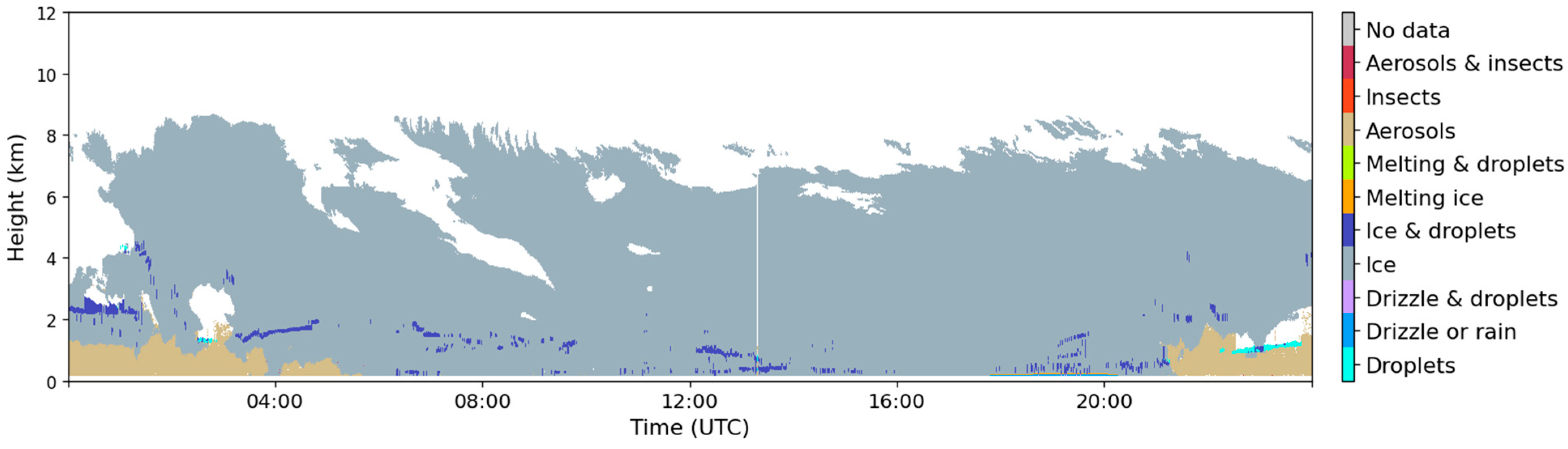
Figure 3 presents the overall atmospheric time-series characterization obtained from the Cloudnet database [
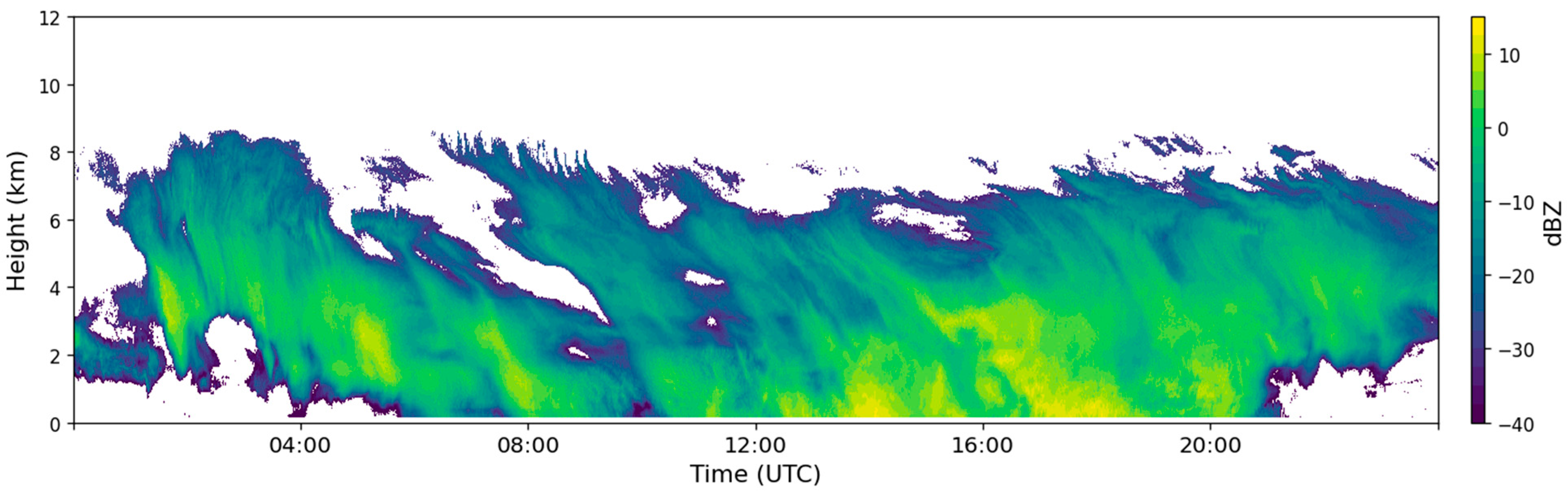
27] using both ceilometer and radar reflectivity factor data. The atmosphere is dominated by large ice cloud particles. It should be noted that, for this application, the ceilometer is generally unsuitable as a data-collecting platform. Additionally, applications related to laminar channels extrapolated in the atmosphere through multifractal theory have only been developed using ceilometer or lidar data so far. The ceilometer is unable to obtain higher altitude data in cloudy conditions due to oversaturation of the backscattered light sensor, as shown in
Figure 4. Therefore, it is necessary to use radar reflectivity factor data, as shown in
Figure 5. This marks the first instance of radar data being employed for laminar channel applications.
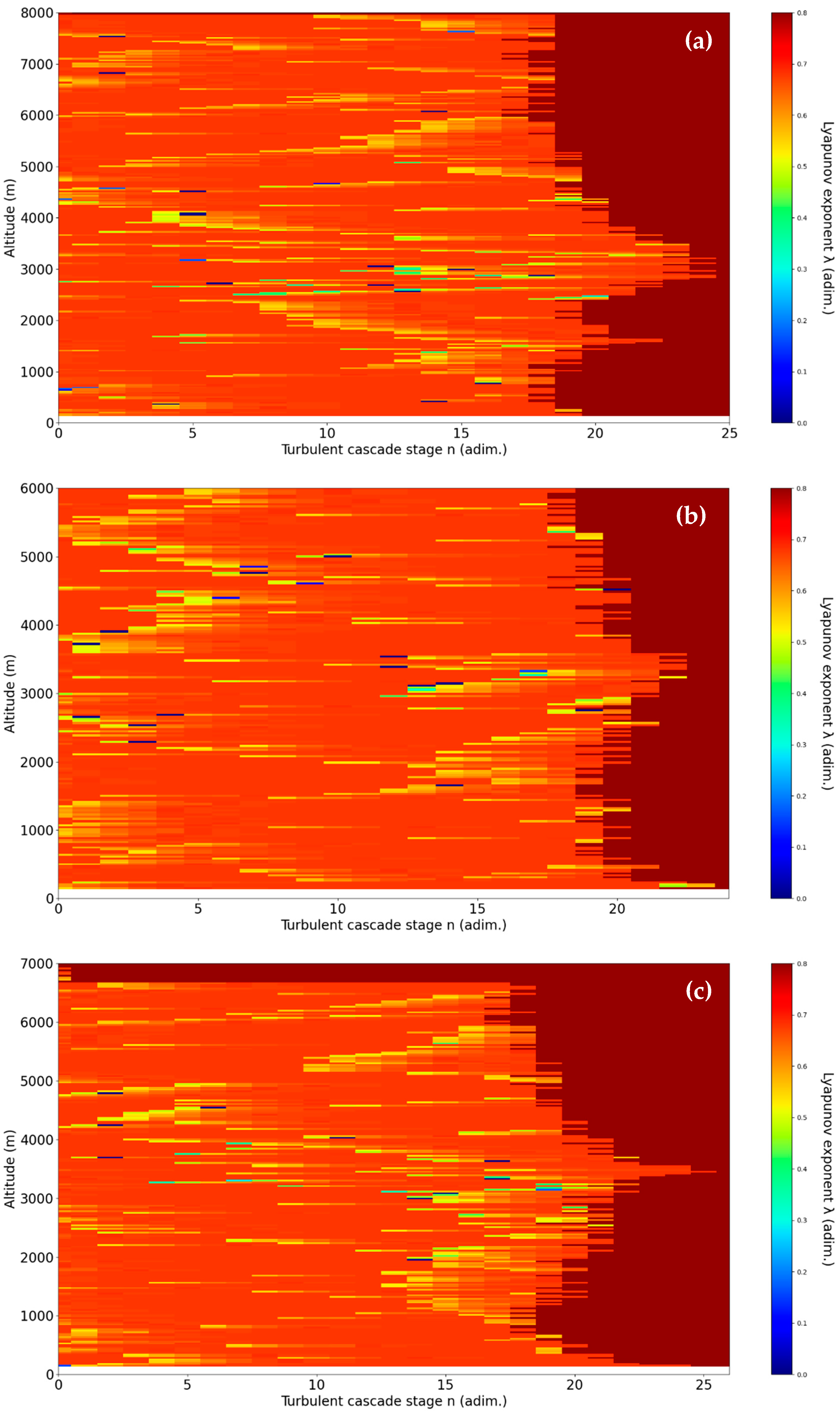
Figure 6a accurately describes the descent of cloud formations through lower altitude descending laminar channels. However, it is interesting to note that weak ascending laminar channels are observed at higher altitudes. The explanation is that in this region, the top of the cloud formation does not descend but exits the profile range of the radar reflectivity factor. In other words, that part of the cloud is ascending in a direction that is not accessible to the radar, and thus it appears to be descending. The laminar analysis proves to be useful in differentiating such cases.
Also, anomalous laminar bands appear in the upper regions, which are representative of the very sudden fluctuations and instabilities which are visible at the top of the cloud in that timeframe in
Figure 4. In any case, it seems that the laminar channel analysis can be used to determine when upper parts of cloud masses exhibit high instability.
In
Figure 6b, in this particular timeframe, atmospheric stability is mostly expected, and this is what the laminar analysis also shows. There is no significant ascending or descending laminar channels.
In
Figure 6c, stability can be seen by the raw data and by the laminar analysis; however, the analysis shows ascending laminar channels at higher altitudes. It is visible, however, that the cloud formation is indeed slightly ascending at higher altitudes in this instance, and thus the laminar analysis correctly predicts atmospheric behaviour. Once again, in the instance analysed in
Figure 6d, we are expecting stability, and stability is indeed found. Another interesting pattern is noticed in the analysis, and it must be explained: the peak that appears in the turbulent cascade stage axis always appears in areas with the largest number of backscattering bodies. This occurs because high numbers of turbulent cascade stages indicate areas of very low dissipation, and thus, in such areas, cloud formations are dissipated much slower and airborne ice densities increase. It is then apparent that the laminar analysis can show which areas of the profile have the most airborne ice.
Figure 6a and
Figure 7 shows an interesting correlation with our model as they demonstrate a significant gradient of ice particle speed at 4:00 at relatively low height, indicating a laminar channel. This is also suggested by the ceilometer and radar reflectivity data, which show an increased backscattering profile at similar heights. This is consistent with the previous described theoretical model (see for example Equation (33), in which it is observed that
is the velocity associated with the laminar–turbulent flow transition, speed that can be assimilated to the sedimentation rate of aerosols, while
corresponds to diffusion deposition speed inversely proportional to
and proportional to
, coefficient assimilated to fractal–nonfractal transition, i.e., the transition from laminar to turbulent flows), which can predicts an increased deposition rate at the transition from laminar to turbulent flows.


 ,
, 


