Article

Ross–Weddell Dipole Critical for Antarctic Sea Ice Predictability in MPI–ESM–HR

by
Davide Zanchettin
1,*,
Kameswarrao Modali
2,
Wolfgang A. Müller
3 and
Angelo Rubino
1
1
Department of Environmental Sciences, Informatics and Statistics, University Ca’Foscari of Venice, Via Torino 155, 30172 Mestre, Italy
2
Deutsches Klimarechenzentrum GmbH (DKRZ), Bundesstraße 45a, D-20146 Hamburg, Germany
3
Max Planck Institute for Meteorology, Bundesstraße 53, D-20146 Hamburg, Germany
*
Author to whom correspondence should be addressed.
Atmosphere 2024, 15(3), 295; https://doi.org/10.3390/atmos15030295
Submission received: 25 January 2024 / Revised: 22 February 2024 / Accepted: 26 February 2024 / Published: 28 February 2024

Abstract

:
We use hindcasts from a state-of-the-art decadal climate prediction system initialized between 1979 and 2017 to explore the predictability of the Antarctic dipole—that is, the seesaw between sea ice cover in the Weddell and Ross Seas, and discuss its implications for Antarctic sea ice predictability. Our results indicate low forecast skills for the Antarctic dipole in the first hindcast year, with a strong relaxation of March values toward the climatology contrasting with an overestimation of anomalies in September, which we interpret as being linked to a predominance of local drift processes over initialized large-scale dynamics. Forecast skills for the Antarctic dipole and total Antarctic sea ice extent are uncorrelated. Limited predictability of the Antarctic dipole is also found under preconditioning around strong warm and strong cold events of the El Niño-Southern Oscillation. Initialization timing and model drift are reported as potential explanations for the poor predictive skills identified.

1. Introduction

Antarctic sea ice forms in the open Southern Ocean around the Antarctica landmass, and its spatio-temporal evolution is largely shaped by equatorward drifting and melting forced by the circumpolar system of southern midlatitude westerly winds and ocean currents. These winds and currents set the northern boundary of Antarctic sea ice and, by limiting anomalous atmospheric and oceanic poleward heat flows, reduce its exposure to global changes [1,2,3]. The Southern Ocean, and the Antarctic circumpolar current in particular, feature large eddy activity and spontaneously generate strong ocean intrinsic variability [4,5,6,7,8]. Accordingly, Antarctic sea ice has displayed modest historical trends in the early satellite era [9,10,11], as its variability was dominated by the seasonal component [12]. The more pronounced Antarctic sea ice extent anomalies observed since the 2000s, especially in the West Antarctic [13,14], have revitalized interest in interannual and decadal variability and the predictability of this critical component of the Earth system [15,16,17,18,19,20]. Even more so, the record minimum extents observed in 2022 and 2023, in concomitance with Southern Ocean subsurface warming, have been portrayed as the first evidence of a new state of Antarctic sea ice [21]. However, despite potential sources of predictability identified in the Pacific [18], Indian [22] and Atlantic sectors [23,24], decadal prediction of Antarctic sea ice remains a challenge for current coupled climate models [25,26].
Interannual variability of Antarctic sea ice is dominated by a seesaw in sea ice distribution encompassing the Ross–Amundsen Seas and Bellingshausen–Weddell Seas, known as the Antarctic dipole (ADP), which mainly represents a standing wave in the western hemisphere of the Antarctic [27]. The ADP index accordingly describes temporal variations in the strength of this seesaw, with positive phases of the index describing concomitant anomalous sea ice cover gains in the Weddell Sea and losses in the Ross Sea, and vice versa for negative phases. The structure and magnitude of this ADP varies seasonally following seasonal changes in the overlying atmospheric circulation anomalies [10].
The ADP is associated with the cyclonic flow around the Amundsen Sea Low [28], where the sea ice dipole is a thermodynamical and dynamical response to the cold equatorward wind over the Ross Sea and the warm poleward winds into the Antarctic Peninsula/Bellingshausen Sea region. Deepening/shallowing or displacement of the Amundsen Sea Low are thus associated with ADP anomalies [29]. Wind-driven ADP and Antarctic sea ice variability and trend have been attributed to several factors, ranging from intrinsic climate variability to external forcing by stratospheric ozone changes or an increase in atmospheric greenhouse gas concentrations [30,31,32]. In addition to local wind forcing, sea ice variability and trends in the key regions of the ADP have been associated with surface freshening and changes in the upper stratification of the Southern Ocean that are triggered by increased precipitation [33] or are part of an ocean-sea ice feedback [34].
Teleconnections have been identified between the ADP and extratropical and tropical variability in the Southern Hemisphere: on interannual time scales, the ADP and Antarctic sea ice variability are intertwined with variability of the storm track in the Southern Hemisphere though a variety of thermodynamical and dynamical mechanisms, and feedbacks that evolve through the austral winter semester [35]. The ADP is associated with the Pacific South American pattern, which is in turn part of the El Niño-Southern Oscillation (ENSO) global teleconnection [36,37,38]. The ENSO-ADP linkage contributes to the host of evidence from observational and climate modelling studies that point to the tropical Pacific having a significant effect on Antarctic sea ice cover [10,11,39,40,41,42].
This study builds on this evidence, which suggests that the ADP index exhibits persistent interannual anomalies (especially after being triggered by ENSO forcing), to assess predictability of the ADP in a state-of-the-art decadal climate prediction system. It attempts to determine if ENSO, and specifically its teleconnection and associated biases, predominate over other sources of variability, including the intrinsic variability of the Southern Ocean dynamics.

2. Materials and Methods

2.1. Decadal Climate Prediction System

This study makes use of the preoperational MiKlip system for decadal climate predictions, which is based on the high-resolution version of the Max Planck Institute—Earth System Model (MPI–ESM–HR) [43]. MPI–ESM–HR is a conglomerate of a coupled general circulation model and subsystem models for land, vegetation, and biogeochemistry. In MPI–ESM–HR, the atmospheric general circulation model ECHAM6 uses a T127/~100 km horizontal resolution and 95 hybrid sigma pressure levels that extend up to 0.01 hPa; the ocean-sea ice model MPIOM [44] uses the TP04 configuration with an eddy-permitting 0.4° global resolution on a tripolar grid with 40 z-levels.
In MPI–ESM, oceanic biases prevail in the intermediate layers of the ocean, which reflects the inability of the model to maintain the correct water mass properties [43,44]. In general, the ocean in MPI–ESM gets too warm and saline at intermediate levels and in the deep ocean, whereas it is too cold and fresh in the upper layers. Antarctic sea ice and its seasonal cycle are generally underestimated in MPI–ESM, which is likely due to a bias in the modeled low-pressure system over the Amundsen Sea, with repercussions for air pressure distribution over the Weddell Sea. MPI–ESM–HR and similar or lower-resolution configurations of MPI–ESM have been widely tested and used in studies of climate dynamics and variability [3,45,46,47], as well as in studies of climate predictability [48,49,50,51].
We use the output of the MiKlip decadal prediction experiments, which are based on full-field assimilation of the ORAS4 ocean reanalysis data [52] contributed to the dcppA experiment of the Decadal Climate Prediction Project (DCPP) [53]. The simulations include a historical assimilation run covering the period November 1958–November 2018, hindcasts initialized on 1 November of each year between 1960 and 2017 and using historical forcing. Each hindcast consists of five ensemble members that differ in the initial state (r1, …, r5). Our analysis is limited to the period 1979–2018, as sea ice values are relaxed toward the climatology before the satellite era, which could be inconsistent with other assimilated data and trigger unrealistic dynamics. The external radiative forcing data are based on the recommendations by the sixth phase of the Coupled Model Intercomparison Project (CMIP6), which [54] provides an overview of.

2.2. Data Preprocessing

The output of MPI–ESM–HR is pre-processed to remove the effects of systematic climate model errors, including drift and bias [48,55,56]. The drift/bias correction method recommended by the DCPP [53] is employed, and is based on empirical estimates that are determined as the mean error of all ensembles, when compared to the assimilation run.
Spatially integrated sea ice cover for different key regions of the Southern Ocean is considered, and specifically, the domains of the Weddell Sea and Ross Sea basins span latitudes ≤60° S at longitudes between 57° W and 12° E (to the coastline), and between 166° E and 155° W (to the coastline), respectively.
The ADP index is calculated as the difference between the spatially-integrated sea ice covers for the Weddell Sea and the Ross Sea.
ENSO is evaluated using the monthly Nino3.4 index, defined as the spatially averaged sea-surface temperature within the domain encompassing 5° S–5° N latitude and 170° W–120° W longitude.

2.3. Statistical Analyses

Forecast skills are estimated using the root mean square error (rmse) and the Persistence Index, as detailed in [57]. The value of the initialization year is used as reference for the calculation of the persistence index.
Trends are estimated using a linear regression with least squares. Time series are detrended separately for each month of the year. Statistical significance of correlations accounts for autocorrelation in the series following [58].
Based on the ADP index, years are clustered into two groups, describing strong positive (upper quartile) and strong negative (lower quartile) values of the index for both March and September values. Unless otherwise specified, the significance of local sea ice concentration anomalies for the so-identified clusters is tested with a rank sum (Mann–Whitney U) test that compares values for each cluster year with those for all other years.

3. Results

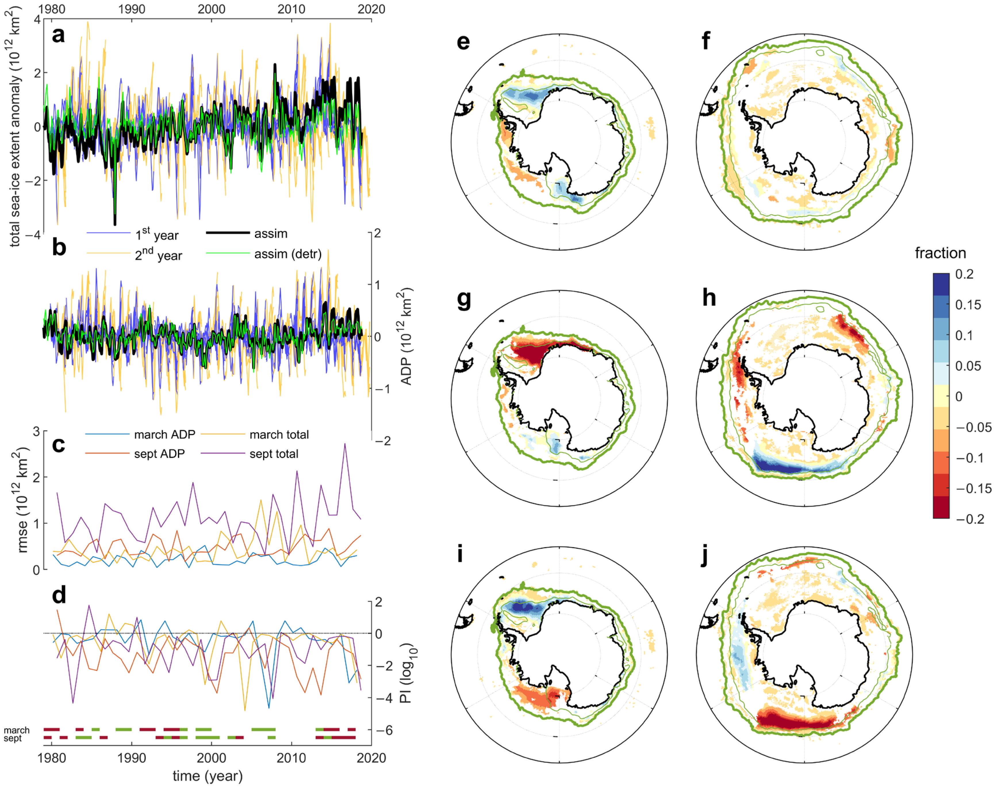
3.1. Antarctic SeaIce Evolution and Predictability

Figure 1 illustrates Antarctic sea ice extent evolution and predictability in the MPI–ESM–HR decadal prediction system. The total Antarctic sea ice extent is characterized by a long-term positive trend and substantial interannual variability, which are both, in overall terms, poorly captured by the hindcasts, as evidenced by the envelope of first and second hindcast year values that widely embed the assimilated time series (Figure 1a). Certain years (most noticeably 1997, 1998, 2010, 2016 and 2018) are clearly affected by systematic errors that exceed the range of observed year-by-year variability and are already developed within the first hindcast year. Accordingly, hindcast skill metrics show substantial year-by-year variability for both March and September extents (Figure 1c). The persistence index resembles the rmse in producing generally poor predictions, with only a few years characterized by positive values, which is indicative of skillful hindcasts (Figure 1d). The analysis confirms strong year-to-year changes in Antarctic sea ice predictability, and highlights the separation of winter and summer dynamics (i.e., a skillful prediction of minimum extent does not guarantee a skillful prediction of the following maximum).
The ADP is characterized by contrasting trends in summer and winter months that describe a progressively enhanced seasonal cycle, and by substantial interannual and decadal variability (Figure 1b). The ADP significantly contributes to year-by-year total sea ice extent variability in September (r = −0.44, p = 0.004 for 1979–2018 detrended series) but less so in March (r = 0.27, p = 0.104 for 1979–2018 detrended series) (Figure 2). Correlations increase for non-detrended time series (r = −0.47, p = 0.002 and r = 0.52, p = 0.018 for September and March, respectively), suggesting a connection between the ADP and total Antarctic sea ice trends. This seasonal connection is confirmed by the pattern of March sea ice concentration trends when it is superimposed on a positive phase of the ADP, with sea ice increase in the Weddell Sea and decrease in the Ross Sea (Figure 1e) contrasting with the weaker and more coherent trends in September in the same basin (Figure 1f). Lead-lag correlations help to establish causal relationships between the ADP and total Antarctic sea ice cover. Figure 2a illustrates the complexity of the interactions through the course of the year, where the ADP leads total sea ice in December, and then lags behind it in late austral summer and autumn. The positive correlations during this period of the year suggest that there is constructive superposition of the regional and circumpolar anomalies. In contrast, as noted above, correlations are generally negative during the austral winter, which is indicative of negative feedbacks; significant values when the ADP leads suggest they originate in sea ice anomalies in the Western Hemisphere. The development of interactions between ADP and sea ice concentrations in austral summer and toward the climatological annual minimum in March highlights dynamics that are internal to the Weddell Sea: in an initial positive phase of the ADP in November, anomalous sea ice gains develop in January to the east of the tip of the Antarctic peninsula, near to the 15% sea ice concentration margin, and then move eastward toward the shelf, reinforcing the positive ADP in February as the sea ice margin shrinks (Figure 2b–e).
A cluster analysis of the Weddell and Ross Seas total sea ice covers describes how both basins contribute to large anomalies of the ADP (Figure 3a–c): For March, both basins contribute to the ADP anomaly, with significantly anomalous gains (losses) in the Weddell (Ross) Sea for positive against negative phases of the ADP. Median differences (1012 km2) are 0.577 for ADP, 0.505 for the Weddell Sea and −0.157 for the Ross Sea. For September, only the Ross Sea exhibits significant differences in sea ice cover between opposite phases of the ADP, whereas the Weddell sea ice cover changes are irrelevant (median differences, in 1012 km2 are 0.248 and 0.025, respectively). There is therefore an asymmetry between the relative roles of Weddell and Ross sea ice cover for the ADP in March and September. The assimilated spatial patterns of sea ice concentration reveal the elements of this asymmetry and suggest that different dynamics operate under strong positive and strong negative phases of the ADP: In March, strong negative ADP highlights strong anomalous sea ice loss in the Weddell Sea (Figure 1g), while strong positive ADP stems from sea ice gain in the Weddell Sea, coupled with sea ice loss in the Ross Sea (Figure 1i); in September, the phase of the ADP appears to strongly relate to anomalous sea ice gain or loss around the sea ice edge in the Ross Sea, while anomalies of the opposite sign relate to the upstream Drake passage, and only produce a weak signature in the Weddell Sea (Figure 1h,j).
In a similar way to total Antarctic sea ice extent, but more recurrently, first year hindcast errors for the ADP can exceed observed year-by-year variability, which is indicative of an overall poor predictive performance (Figure 1b). The ADP also exhibits strong year-by-year variations in predictability, as seen in skill metrics that include rmse and persistence index (Figure 1c,d), with no correlation between skills for the ADP and for total sea ice extent. Clustering years based on strong positive and strong negative values of the ADP (Figure 1d) does not reveal a dependency of skills on the state of the ADP, in either March or September (rank sum tests performed on rmse and the persistence index yield non-significant results).
For March, first year hindcasts display a strong relaxation of the ADP and both Weddell and Ross sea ice cover anomalies toward the climatology, as shown by the box-whisker plots shrunk around the zero value for both the positive and negative ADP clusters (Figure 3a–c). The difference between hindcast medians has an opposite sign, compared to the assimilation of the ADP and the Ross sea ice cover, estimated as −0.202 1012 km2 and 0.085 1012 km2, respectively. The associated anomalous patterns confirm the ubiquitous weakness of Antarctic sea ice concentration anomalies in hindcasts around strong anomalous phases of the ADP (Figure 3g,i). For September, the ADP clusters yield hindcasts that are characterized by a large spread, most often crossing the zero value within the interquartile range (Figure 3a–c). In the hindcasts, the ADP clusters are not significantly different, but do have anomalies with opposite sign than in the assimilated data. This tendency is sharper for Ross sea ice concentration (Figure 3c), where the two clusters are significantly different at p = 0.1. Patterns of sea ice concentration anomalies reveal that the Ross Sea tendency stems from a competition between sea ice loss in the interior and sea ice gain in the exterior portions of the basin (Figure 3h,j). In hindcasts, the largest sea ice concentration difference between positive and negative ADP conditions is an extensive and strong loss, with a sea ice fraction anomaly in excess of −0.2, to the east of the Weddell Sea within the 15% sea ice concentration margin.
There seems to be an interplay between difficulties in predicting ADP anomalies and sea ice cover trends. In March, tendential sea ice growth occurs especially in the Weddell and eastern Ross Seas, which is partly compensated by losses in the Bellinghausen Sea (Figure 1e); this is similar to what was observed for ADP anomalies, where trends in hindcasts are much smaller (about one order of magnitude) and the associated spatial pattern only weakly superposes on the assimilated counterpart (Figure 3e). In September, significant sea ice cover trends are weak, with a sparse circumpolar distribution (Figure 1f); trends in hindcasts show a more structured spatial pattern, with a tripole over the Weddell Sea and eastwards of it (Figure 3f). Overall, when compared to assimilated data, the magnitude of changes in hindcasts appear to be smaller in March and larger in September.

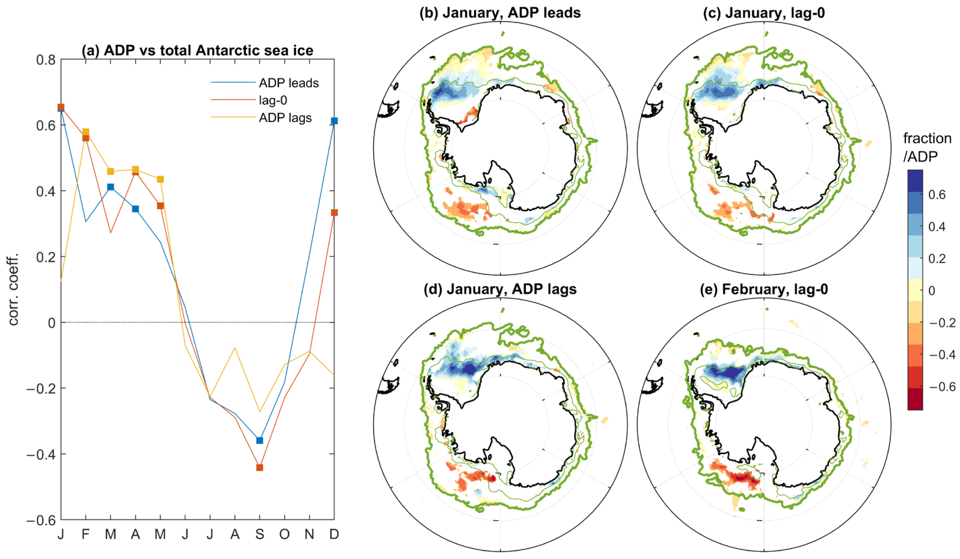
3.2. Teleconnections and Sea Ice Predictability

Figure 4 compares the evolution of Antarctic sea ice concentration, sea surface temperature and atmospheric circulation anomalies under strong positive March ADP phases, both in the assimilation run and in the hindcasts. There is substantial agreement between hindcasts and assimilated data from the first hindcast month (November), with a seesaw between anomalous sea ice gain in the western Weddell/Bellinghausen/Somov Seas and loss in the Ross Sea, which is superposed on a zonal wave train with negative upper tropospheric geopotential height anomalies over the Amundsen Sea, and consistent El Niño-like sea surface temperature anomalies (Figure 4a,f). In the assimilation, these sea ice concentration anomalies weaken in the following months, and persist in the hindcasts (at fraction anomalies around or in excess of 0.2), especially in the Bellinghausen Sea, where sea ice is largely overestimated in December and January (Figure 4b–d,g–i).
At this stage, the patterns of sea surface temperature anomalies show better consistency than sea ice between assimilated and hindcast data, although the latter feature a stronger meridional tripole in the Nino3.4 longitudinal band, encompassing positive anomalies at the equator and mid-latitudes, and negative anomalies in the tropics. Concomitantly, the atmospheric wave anomaly moves westward while dampening, with the negative geopotential height anomalies found over the Ross Sea in December becoming non-significant over the sea ice domain in January. We argue that in the hindcasts the wave remains strong and stationary, contributing to the erroneous persistence of the initialized sea ice anomalies. In February and March, the positive ADP pattern is fully developed in assimilated data, concomitant with a clear El Niño anomaly (Figure 4d,e). In contrasting the earlier months with February and March, the hindcasts show weaker sea ice and sea surface temperature anomalies than assimilated data (Figure 4i,j), yielding the vanishing sea ice concentration anomalies already observed in Figure 3i. The overall impression is that when hindcasts are compared to assimilated data they are seen to be characterized by a weaker imprint of large-scale dynamics and a predominance of a slow local relaxation of initialized conditions toward the climatology.

3.3. Model Drift

Figure 5 illustrates the month-by-month evolution of Antarctic sea ice concentration drift, up until March of the first hindcast year. In the first hindcast month, the drift already causes a ubiquitous sea ice loss around Antarctica, with locally large values exceeding 10% of the grid area, especially in the eastern Weddell Sea and in the west of the Ross Sea (Figure 5a). In the following months, this systematic erroneous sea ice loss moves toward the central portions of the Weddell and Ross Seas where, in concomitance with the seasonal shrinking of the sea ice margin, it strengthens up to an underestimation of sea ice cover that is more than 30% than the amount in assimilated data (Figure 5b,c). In March, the regions characterized by the strongest drift correspond to the ADP key regions in the Ross and Weddell Seas (compare Figure 5e with Figure 1g,i). Accordingly, despite the drift being removed from hindcasts in the post-processing of the model output, the associated systematic erroneous local sea ice loss appears to predominate over other dynamics, and leads toward a fast dampening of initialization constraints.

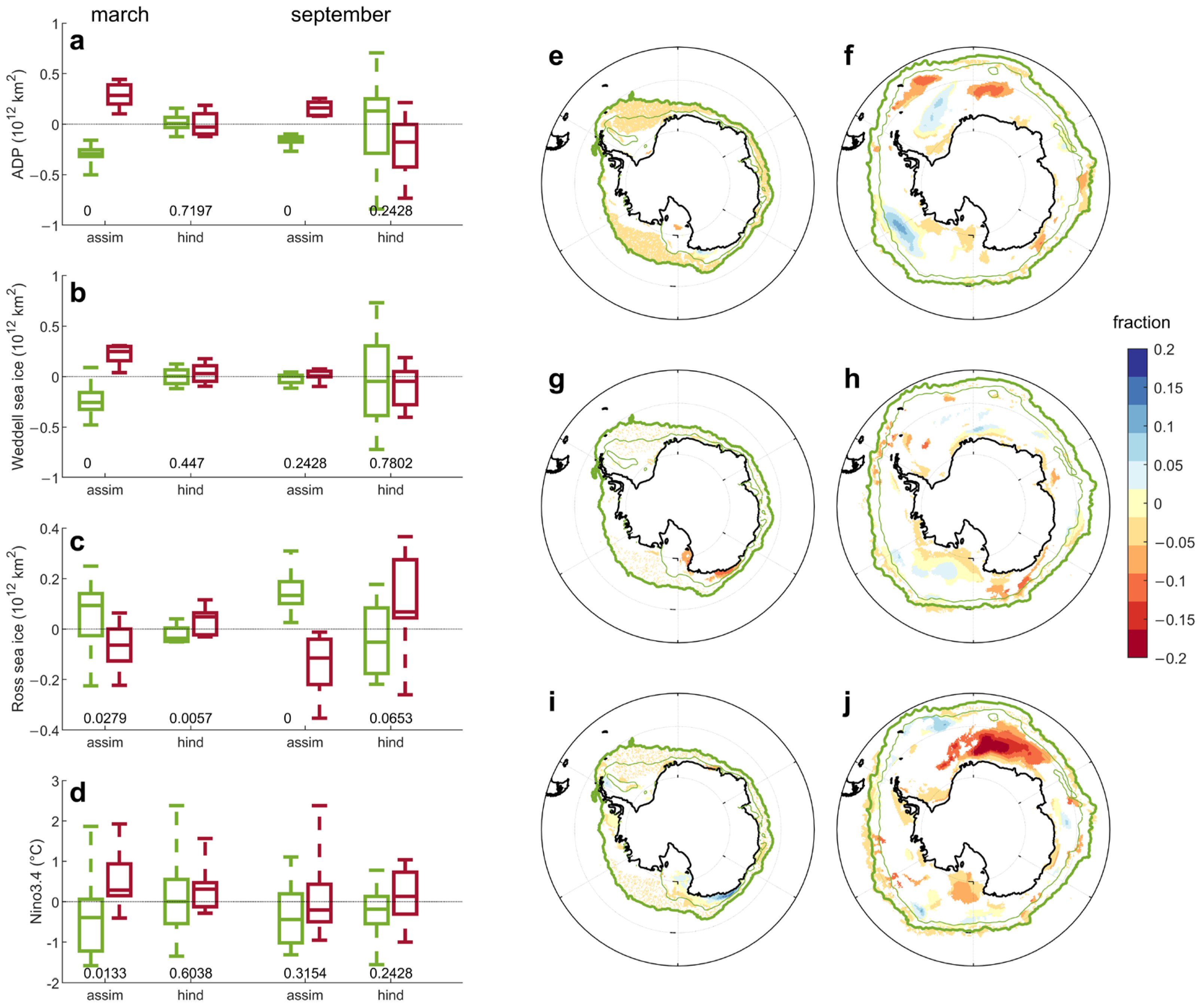
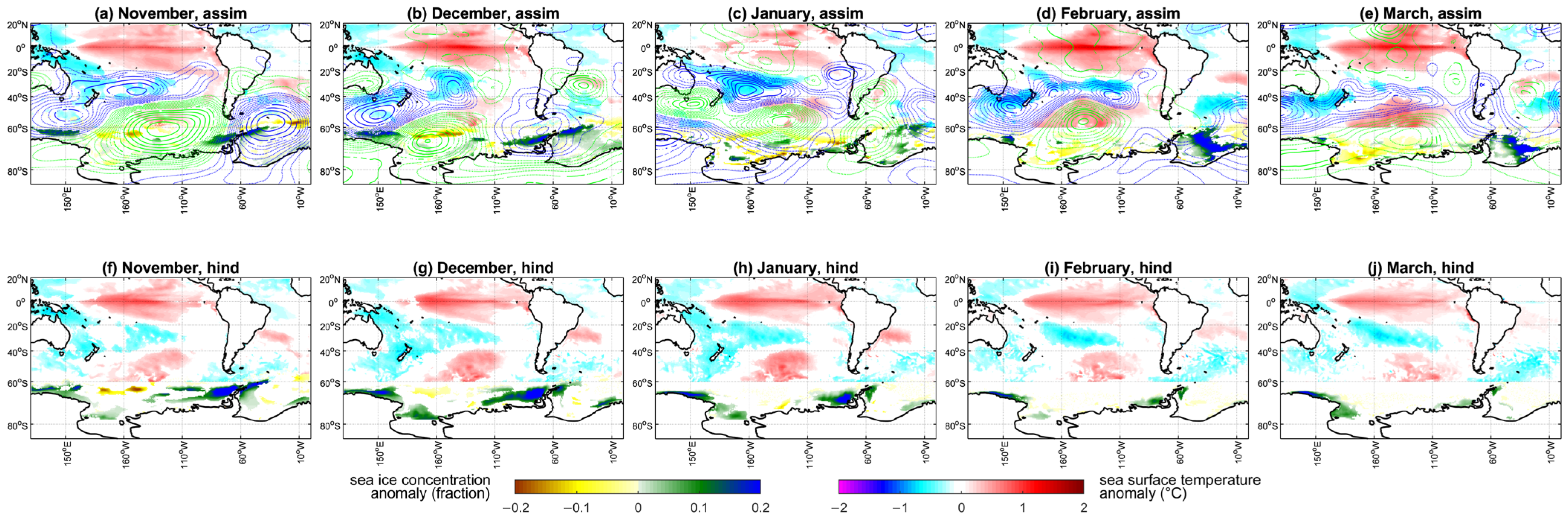
3.4. ENSO as a Source of ADP Predictability

ENSO is a known forcing factor of ADP variability, which is confirmed here by the significantly different ENSO state for strong positive and strong negative phases of the ADP in March, which correspond to prevalent El Niño- and La Niña-like anomalies, respectively (Figure 3d). Specifically, the median of the Nino3.4 index in strong (negative) positive ADP phases is +0.28 °C (−0.39 °C). However, compared to assimilated data, the hindcasts largely underestimate ENSO anomalies in March, with largely overlapping distributions of the Nino3.4 index (+0.31 and +0.001 °C in strong positive and strong negative phases of the ADP, respectively) yielding non-significant ENSO differences (Figure 3d). Since this corresponds to a failure of the ADP forecast (Figure 3a–c and Figure 4e,j), we are led to question the extent to which the lack of predictability in the ADP can be attributed to the weak skill of ENSO predictions.
Figure 6 illustrates the evolution in assimilation and hindcasts of ENSO and Antarctic sea ice anomalies around the occurrence of major El Niños (first hindcast March in 1983, 1992, 1998, 2010, 2016) and La Niñas (first hindcast March in 1985, 1989, 2000, 2008, 2011). In assimilated data related to major El Niño and La Niña events, ENSO remains in a significantly different state from the May preceding to the June following the peak of the event (black squares in Figure 6d). Hindcasts show an even longer persistence of differences, with both ensemble mean and individual hindcasts (grey squares in Figure 6d) lasting up to one year after the peak of the event and reemerging in the following austral autumn (mostly related to enduring warm conditions following El Niños, and to a stronger shift to El Niño-like anomalies one year after La Niñas—see Figure 6d). Specifically, at around the peak of the El Niños, defined as the December–February average, the ensemble average of the Nino3.4 anomaly for all El Niño events is 2.33 °C for the assimilation and 1.95 °C for the hindcasts; in the following austral winter, defined as the June–August average, the ensemble average for all El Niño events is −0.32 °C for the assimilation and 0.60 °C for the hindcasts.
The ADP shows significant differences only before the peak of El Niño/La Niña, a feature which is only captured by predictions in the first hindcast month (November of Year 0) (Figure 6a). In March of the first hindcast year, the ensemble average of the ADP anomaly for all El Niño (La Niña) events is 0.044 (−0.115), 1012 km2 in the assimilation and 0.011 (−0.016) 1012 km2 in the hindcasts. Instead, the ADP is significantly different in the two autumns/winters following the peak of El Niño/La Niña, with a good overlap with the development of too warm El Niño conditions. The ensemble average of the ADP anomaly for all El Niño (La Niña) events in the austral winter following the peak of the event is −0.048 (−0.027), 1012 km2 for the assimilation and −0.057 (0.091) 1012 km2 for the hindcasts. The large forecast spread during these periods however indicates the low signal-to-noise ratio of simulated ENSO influences on the ADP.
Analysis of clusters of Weddell and Ross Sea ice covers further complicates a robust attribution of ADP anomalies around major ENSO events. The assimilated data already only show significant differences sporadically, most noticeably for Ross Sea sea ice cover in the austral winter preceding the peak of El Niño/La Niña (Figure 6b,c), which however strongly depended on one event (the 2008 La Niña). Hindcasts show significant differences in the Weddell Sea during the first hindcast year (sporadic), and in the Ross Sea during the second hindcast year. Finally, this suggests that multiple mechanisms acting on the two characteristic basins of the ADP contribute to its apparent predictability being conditioned to ENSO.

4. Discussion

Our study adds to the host of recent scientific evidence [16,17,18,25,26,59] that especially highlight Antarctic sea ice and the Antarctic dipole as critical aspects of near-term climate variability and predictability, especially in the austral summer season [26,60]. The stark contrast between the large and extensive assimilated sea ice anomalies, clustered by construction around opposite phases of the ADP, and the lack of responses in the corresponding predicted values describes the limited predictability of these components of Antarctic sea ice variability in our model setup. According to our analysis, this limited predictability of the ADP holds even around strong ENSO events, which have previously been identified as a major remote source of ADP variability [10,36,37,38]. Since assimilated data indicate ENSO as a source of ADP variability and hindcasts indicate predictability for ENSO, at least in contrasting major El Niños and La Niñas, the lack of ADP predictability under strong ENSO events implies that other factors dominate over the ENSO forcing.
Among the possible causes of the poor forecast skills are a predictability barrier linked to the timing of initialization and the erroneous representation in the model of oceanic and atmospheric processes—or more generally of the interactions and feedbacks in the climate system. The hindcast initialization in November implies that ENSO anomalies are well developed, as El Niños typically reach their mature phase in boreal winter [61]; however, other precursors of Antarctic sea ice variability, especially the southern annular mode [62,63,64], might not be well constrained. Also, Antarctic sea ice mostly responds to large-scale modes during the austral cold season [10], and the limited predictability evidenced here may therefore arise from several months of growing errors in sea ice precursors, since the initialization in late austral spring until the teleconnection is fully established. These growing errors may disrupt the seasonal asymmetry between the ADP and total Antarctic sea ice, where austral summer is characterized by constructive superposition of anomalies and winter by anticorrelation. The effects of initialization timing remain difficult to quantify based on our results, as this would require additional hindcasts initialized at different times over the year.
The long-lasting differences between clusters of hindcasts initialized around strong warm and cold phases of ENSO may support the recently suggested potential for multi-year predictability of ENSO [65]. However, caveats to our analysis include consideration of only the strongest ENSO events, a weak threshold for statistical significance and possible biases in ENSO oscillatory dynamics. Further investigation is therefore required before concluding that MPI–ESM–HR features a broader window of opportunity for ENSO prediction beyond the spring predictability barrier.
Concerning systematic errors, Antarctic sea ice is generally underestimated in MPI–ESM, and is affected by a poor representation of the observed seasonal cycle [44]. As shown here, the model’s drift toward the biased Antarctic sea ice climatology is rapid following the initialization, with substantial errors diagnosed already in the first hindcast month and further reinforced in the following months, concomitant with the seasonal sea ice shrinking during austral spring and summer. This underestimation appears to contribute to an artificial ADP dampening, as also shown by a multi-model analysis of global warming scenario experiments, in which reduced Antarctic sea ice weakens the ADP variability [66]. Furthermore, model drifts toward this biased climatology are known to dynamically interfere with hindcast signals, residuals and background climate, critically contributing to uncertainty in decadal climate predictions [48]. Due to the drift, artificial anomalies in sea ice concentration can reach values of −40% in the Weddell Sea in the first March following initialization (Figure 5e), a value that is comparable to, or even locally exceeds, the expected difference between assimilated positive and negative phases of the ADP (Figure 1g,i). Accordingly, hindcasts produce vanishing sea ice concentration anomalies (Figure 3g,i) as the drift overwhelms other signals. This suggests that the drift is the dominant factor contributing to lack of ADP predictability in austral summer in our hindcasts. The mechanism underlying Antarctic sea ice drift is unidentified, but arguably involves thermodynamic processes linked to the warm surface bias in the Southern Ocean, detected in this and lower resolution versions of MPI–ESM [43]. Also, current climate models share a bias in Antarctic sea ice thickness, which calls for improvements in sea ice dynamics as well [67].
Lack of realism in the simulation of the seasonal phase-locking of ENSO (as shown in lower resolution versions of MPI–ESM in [44]) may have profound dynamical implications for the ADP during the drifting phase of the hindcasts, especially during austral spring [11]. Similar concerns arise in relation to the spatial patterns of ENSO, as the bulk of ENSO activity in MPI–ESM–HR is constrained to the central Pacific [43] and may lack the variety of ENSO flavors and associated teleconnections shown in observations [68,69,70]. Beyond biases in ENSO, the various potential mechanisms of tropical forcing of high-latitude processes relevant to the ADP may suffer from a biased simulated representation. The underexplored remote sources of Antarctic sea ice variability include the tropical Atlantic [23,24]. In this regard, our analysis of ADP highlights (for hindcasts but not assimilated data) extensive and strong sea ice concentration anomalies to the east of the Weddell Sea that call for further investigations of Atlantic–Antarctic teleconnections.
Southern Ocean dynamics, and especially their predominant intrinsic component [5,6,7], can also critically affect Antarctic sea ice variability and predictability. Purely intrinsic ocean dynamics cannot be disentangled from the atmospheric driven component of our coupled model system; yet clustering strong and weak states of Southern Ocean total surface kinetic energy—a common diagnostic of intrinsic ocean variability—indicates lack of predictability within a few months of initialization, due to the large ensemble spread of the hindcasts (not shown). MPI–ESM–HR may significantly overestimate the strength of the Antarctic circumpolar current [43], which would affect the simulated representation of intrinsic ocean variability as well [7]. Overall, this calls for improved understanding and simulation of fundamental processes that can drive ocean variability, both locally as well as remotely. Beyond dedicated sensitivity experiments to disentangle the relative roles of the various sources of Antarctic sea ice variability, the large spread diagnosed in some quantities calls for larger ensembles of hindcasts that will work toward robust Antarctic sea ice predictions, even under strong preconditioning.

5. Conclusions

This study describes the low forecast skills of the Antarctic sea ice dipole in the first hindcast year demonstrated by a decadal climate prediction system based on the MPI–ESM–HR model. In the hindcasts, which are initialized at the beginning of November, sea ice concentration in the core regions for the Antarctic dipole quickly relaxes toward the climatology, even under strong forcing from Antarctic dipole predictors, such as a strong El Niño. This model drift, systematically inducing erroneous sea ice concentration anomalies of up to −40% in the Weddell Sea within five months of initialization, overwhelms predictable sea ice signals, especially in austral summer. The drift is thus the main factor determining the lack of predictability of the Antarctic dipole and total Antarctic sea ice in this model setup. Our study calls for a stronger research focus on the sources of Antarctic sea ice drifts and biases, including their seasonal evolution.

Author Contributions

Conceptualization, D.Z.; methodology, D.Z.; validation, D.Z.; formal analysis, D.Z.; investigation, D.Z.; data curation, D.Z.; writing—original draft preparation, D.Z.; writing—review and editing, A.R., K.M. and W.A.M.; visualization, D.Z.; funding acquisition, D.Z. and A.R.; revision: D.Z. All authors have read and agreed to the published version of the manuscript.

Funding

This research contributes to the project IPSODES (‘Investigating the predictability of the Southern Ocean dynamics through ensemble simulation hindcasts’), which was funded by the “Programma Nazionale di Ricerca in Antartide”—PNRA (project identifier: PNRA18_00199).

Institutional Review Board Statement

Not applicable.

Informed Consent Statement

Not applicable.

Data Availability Statement

All data used in this study are available from the Earth System Grid Federation. A subset of the data is available from the repository at: https://doi.org/10.5281/zenodo.7415692 (accessed on 25 February 2024).

Acknowledgments

Ricardo Viana Barreto contributed to data retrieval and pre-processing. We would like to thank the German Climate Computing Centre (DKRZ) for providing their computing resources to the MiKlip project.

Conflicts of Interest

The authors declare no conflicts of interest.

References

  1. Zhang, J. Increasing Antarctic Sea Ice under Warming Atmospheric and Oceanic Conditions. J. Clim. 2007, 20, 2515–2529. [Google Scholar] [CrossRef]
  2. Zhang, J. Modeling the Impact of Wind Intensification on Antarctic Sea Ice Volume. J. Clim. 2014, 27, 202–214. [Google Scholar] [CrossRef]
  3. Zanchettin, D.; Bothe, O.; Timmreck, C.; Bader, J.; Beitsch, A.; Graf, H.-F.; Notz, D.; Jungclaus, J.H. Inter-hemispheric asymmetry in the sea-ice response to volcanic forcing simulated by MPI-ESM (COSMOS-Mill). Earth Syst. Dyn. 2014, 5, 223–242. [Google Scholar] [CrossRef]
  4. Hogg, A.M.; Blundell, J.R. Interdecadal variability of the Southern Ocean. J. Phys. Oceanogr. 2006, 36, 1626–1645. [Google Scholar] [CrossRef]
  5. Sérazin, G.; Penduff, T.; Grégorio, S.; Barnier, B.; Molines, J.-M.; Terray, L. Intrinsic Variability of Sea Level from Global Ocean Simulations: Spatiotemporal Scales. J. Clim. 2015, 28, 4279–4292. [Google Scholar] [CrossRef]
  6. Wilson, C.; Hughes, C.W.; Blundell, J.R. Forced and intrinsic variability in the response to increased wind stress of an idealized Southern Ocean. J. Geophys. Res. Oceans 2015, 120, 113–130. [Google Scholar] [CrossRef]
  7. Sgubin, G.; Pierini, S.; Dijkstra, H.A. Intrinsic variability of the Antarctic Circumpolar Current system: Low- and high-frequency fluctuations of the Argentine Basin flow. Ocean Sci. 2014, 9, 201–213. [Google Scholar] [CrossRef]
  8. O’Kane, T.J.; Matear, R.J.; Chamberlain, M.A.; Risbey, J.S.; Sloyan, B.M.; Horenko, I. Decadal variability in an OGCM Southern Ocean: Intrinsic modes, forced modes and metastable states. Ocean Model. 2013, 69, 1–21. [Google Scholar] [CrossRef]
  9. Stammerjohn, S.E.; Martinson, D.G.; Smith, R.C.; Yuan, X.; Rind, D. Trends in Antarctic annual Sea Ice retreat and advance and their relation to El Niño-Southern Oscillation and Southern Annular Mode variability. J. Geophys. Res. 2008, 113, C03S90. [Google Scholar] [CrossRef]
  10. Simpkins, G.R.; Ciasto, L.M.; Thompson, D.W.J.; England, M.H. Seasonal relationships between large-scale climate variability and Antarctic sea ice concentration. J. Clim. 2012, 25, 5451–5469. [Google Scholar] [CrossRef]
  11. Fan, T.; Deser, C.; Schneider, D.P. Recent Antarctic sea ice trends in the context of Southern Ocean surface climate variations since 1950. Geophys. Res. Lett. 2014, 41, 2419–2426. [Google Scholar] [CrossRef]
  12. Himmich, K.; Vancoppenolle, M.; Madec, G.; Sallée, J.-B.; Holland, P.R.; Lebrun, M. Drivers of Antarctic sea ice advance. Nat. Commun. 2023, 14, 6219. [Google Scholar] [CrossRef]
  13. Yuan, N.; Ding, M.; Ludescher, J.; Bunde, A. Increase of the Antarctic Sea Ice Extent is highly significant only in the Ross Sea. Sci. Rep. 2017, 7, 41096. [Google Scholar] [CrossRef]
  14. Parkinson, C.L. A 40-y record reveals gradual Antarctic sea ice increases followed by decreases at rates far exceeding the rates seen in the Arctic. Proc. Natl. Acad. Sci. USA 2019, 116, 14414–14423. [Google Scholar] [CrossRef]
  15. Morioka, Y.; Behera, S.K. Remote and local processes controlling decadal sea ice variability in the Weddell Sea. J. Geophys. Res.-Oceans 2021, 126, e2020JC017036. [Google Scholar] [CrossRef]
  16. Libera, S.; Hobbs, W.; Klocker, A.; Meyer, A.; Matear, R. Ocean-Sea Ice Processes and Their Role in Multi-Month Predictability of Antarctic Sea Ice. Geophys. Res. Lett. 2022, 49, e2021GL097047. [Google Scholar] [CrossRef]
  17. Eayrs, C.; Li, X.; Raphael, M.N.; Holland, D.M. Rapid decline in Antarctic sea ice in recent years hints at future change. Nat. Geosci. 2021, 14, 460–464. [Google Scholar] [CrossRef]
  18. Liu, Y.; Sun, C.; Li, J.; Kucharski, F.; Di Lorenzo, E.; Adnan Abid, M.; Li, X. Decadal oscillation provides skillful multiyear predictions of Antarctic sea ice. Nat. Commun. 2023, 14, 8286. [Google Scholar] [CrossRef]
  19. Zhang, L.; Delworth, T.L.; Yang, X.; Zeng, F.; Lu, F.; Morioka, Y.; Bushuk, M. The relative role of the subsurface Southern Ocean in driving negative Antarctic Sea ice extent anomalies in 2016–2021. Comm. Earth Environ. 2022, 3, 2662–4435. [Google Scholar] [CrossRef]
  20. Massonnet, F.; Barreira, S.; Barthé lemy, A.; Bilbao, R.; Blanchard-Wrigglesworth, E.; Blockley, E.; Bromwich, D.H.; Bushuk, M.; Dong, X.; Goessling, H.F.; et al. SIPN South: Six years of coordinated seasonal Antarctic sea ice predictions. Front. Mar. Sci. 2023, 10, 1148899. [Google Scholar] [CrossRef]
  21. Purich, A.; Doddridge, E.W. Record low Antarctic sea ice coverage indicates a new sea ice state. Commun. Earth Environ. 2023, 4, 314. [Google Scholar] [CrossRef]
  22. Yu, L.; Zhong, S.; Vihma, T.; Sui, C.; Sun, B. The Impact of the Indian Ocean Basin Mode on Antarctic Sea Ice Concentration in Interannual Time Scales. Geophys. Res. Lett. 2022, 49, e2022GL097745. [Google Scholar] [CrossRef]
  23. Li, X.; Holland, D.M.; Gerber, E.P.; Yoo, C. Impacts of the north and tropical Atlantic Ocean on the Antarctic Peninsula and sea ice. Nature 2014, 505, 538–542. [Google Scholar] [CrossRef]
  24. Morioka, Y.; Zhang, L.; Delworth, T.L.; Yang, X.; Zeng, F.; Nonaka, M.; Behera, S.K. Multidecadal variability and predictability of Antarctic sea ice in the GFDL SPEAR_LO model. Cryosphere 2023, 17, 5219–5240. [Google Scholar] [CrossRef]
  25. Yang, C.-Y.; Liu, J.; Hu, Y.; Horton, R.M.; Chen, L.; Cheng, X. Assessment of Arctic and Antarctic sea ice predictability in CMIP5 decadal hindcasts. Cryosphere 2016, 10, 2429–2452. [Google Scholar] [CrossRef]
  26. Morioka, Y.; Iovino, D.; Cipollone, A.; Masina, S.; Behera, S.K. Decadal Sea Ice Prediction in the West Antarctic Seas with Ocean and Sea Ice Initializations. Commun. Earth Environ. 2022, 3, 189. [Google Scholar] [CrossRef]
  27. Yuan, X.J.; Martinson, D.G. The Antarctic dipole and its predictability. Geophys. Res. Lett. 2001, 28, 3609–3612. [Google Scholar] [CrossRef]
  28. Hosking, J.S.; Orr, A.; Marshall, G.J.; Turner, J.; Phillips, T. The Influence of the Amundsen-Bellingshausen Seas Low on the Climate of West Antarctica and Its Representation in Coupled Climate Model Simulations. J. Clim. 2013, 26, 6633–6648. [Google Scholar] [CrossRef]
  29. Hobbs, W.R.; Massom, R.; Stammerjohn, S.; Reid, P.; Williams, G.; Meier, W. A review of recent changes in Southern Ocean sea ice, their drivers and forcings. Glob. Planet. Chang. 2014, 143, 228–250. [Google Scholar] [CrossRef]
  30. Haumann, F.A.; Notz, D.; Schmidt, H. Anthropogenic influence on recent circulation-driven Antarctic sea ice changes. Geophys. Res. Lett. 2014, 41, 8429–8437. [Google Scholar] [CrossRef]
  31. Purich, A.; Cai, W.; England, M.H.; Cowan, T. Evidence for link between modelled trends in Antarctic sea ice and underestimated westerly wind changes. Nat. Commun. 2016, 7, 10409. [Google Scholar] [CrossRef]
  32. Ferreira, D.; Marshall, J.; Bitz, C.M.; Solomon, S.; Plumb, A. Antarctic ocean and sea ice response to ozone depletion: A two-time-scale problem. J. Clim. 2015, 28, 1206–1226. [Google Scholar] [CrossRef]
  33. Liu, J.; Curry, J.A. Accelerated warming of the Southern Ocean and its impacts on the hydrological cycle and sea ice. Proc. Natl. Acad. Sci. USA 2010, 107, 14987–14992. [Google Scholar] [CrossRef]
  34. Lecomte, O.; Goosse, H.; Fichefet, T.; Lavergne, C.D.; Barthélemy, A.; Zunz, V. Vertical ocean heat redistribution sustaining sea-ice concentration trends in the Ross Sea. Nat. Commun. 2014, 8, 258. [Google Scholar] [CrossRef]
  35. Zhang, L.; Ren, X.; Wang, C.Y.; Gan, B.; Wu, L.; Cai, W. An observational study on the interactions between storm tracks and sea ice in the Southern Hemisphere. Clim. Dyn. 2024, 62, 17–36. [Google Scholar] [CrossRef]
  36. Yuan, X. ENSO-related impacts on Antarctic sea ice: A synthesis of phenomenon and mechanisms. Antarct. Sci. 2004, 16, 415–425. [Google Scholar] [CrossRef]
  37. Yuan, X.J.; Li, C.H. Climate modes in southern high latitudes and their impacts on Antarctic sea ice. J. Geophys. Res. 2008, 113, C06S91. [Google Scholar] [CrossRef]
  38. Zhang, C.; Li, T.; Li, S. Impacts of CP and EP El Niño Events on the Antarctic Sea Ice in Austral Spring. J. Clim. 2021, 34, 9327–9348. [Google Scholar] [CrossRef]
  39. Meehl, G.A.; Arblaster, J.M.; Bitz, C.M.; Chung, C.T.Y.; Teng, H. Antarctic sea-ice expansion between 2000 and 2014 driven by tropical Pacific decadal climate variability. Nat. Geosc. 2016, 9, 590–595. [Google Scholar] [CrossRef]
  40. Purich, A.; England, M.H.; Cai, W.; Chikamoto, Y. Tropical Pacific SST drivers of recent Antarctic sea ice trends. J. Clim. 2016, 29, 8931–8948. [Google Scholar] [CrossRef]
  41. Turner, J. The El Niño-Southern Oscillation and Antarctica. Int. J. Climatol. 2004, 24, 1–31. [Google Scholar] [CrossRef]
  42. Isaacs, F.E.; Renwick, J.A.; Mackintosh, A.N.; Dadic, R. ENSO Modulates Summer and Autumn Sea Ice Variability Around Dronning Maud Land, Antarctica. J. Geophys. Res. Atmos. 2021, 126, e2020JD033140. [Google Scholar] [CrossRef]
  43. Müller, W.A.; Jungclaus, J.H.; Mauritsen, T.; Baehr, J.; Bittner, M.; Budich, R.; Bunzel, F.; Esch, M.; Ghosh, R.; Haak, H.; et al. A Higher-resolution Version of the Max Planck Institute Earth System Model (MPI-ESM1.2-HR). J. Adv. Model. Earth Syst. 2018, 10, 1383–1413. [Google Scholar] [CrossRef]
  44. Jungclaus, J.H.; Fischer, N.; Haak, H.; Lohmann, K.; Marotzke, J.; Matei, D.; Mikolajewicz, U.; Notz, D.; von Storch, J.S. Characteristics of the ocean simulations in the Max Planck Institute Ocean Model (MPIOM) the ocean component of the MPI-Earth system model. J. Adv. Model. Earth Syst. 2013, 5, 422–446. [Google Scholar] [CrossRef]
  45. Moreno-Chamarro, E.; Zanchettin, D.; Lohman, K.; Jungclaus, J.H. An abrupt weakening of the subpolar gyre as trigger of Little Ice Age-type episodes. Clim. Dyn. 2017, 48, 727–744. [Google Scholar] [CrossRef]
  46. Gutjahr, O.; Putrasahan, D.; Lohmann, K.; Jungclaus, J.H.; von Storch, J.S.; Brüggemann, N.; Haak, H.; Stössel, A. Max Planck Institute Earth System Model (MPI-ESM1.2) for the High-Resolution Model Intercomparison Project (HighResMIP). Geosci. Model Dev. 2019, 12, 3241–3281. [Google Scholar] [CrossRef]
  47. Zanchettin, D.; Fang, S.-W.; Khodri, M.; Omrani, N.-E.; Rubinetti, S.; Rubino, A.; Timmreck, C.; Jungclaus, J.H. Thermohaline patterns of intrinsic Atlantic Multidecadal Variability in MPI-ESM-LR. Clim. Dyn. 2023, 61, 2371–2393. [Google Scholar] [CrossRef]
  48. Zanchettin, D.; Gaetan, C.; Arisido, M.W.; Modali, K.; Toniazzo, T.; Keenlyside, N.; Rubino, A. Structural decomposition of decadal climate prediction errors: A Bayesian approach. Sci. Rep. 2017, 7, 12862. [Google Scholar] [CrossRef]
  49. Schuster, M.; Grieger, J.; Richling, A.; Schartner, T.; Illing, S.; Kadow, C.; Müller, W.A.; Pohlmann, H.; Pfahl, S.; Ulbrich, U. Improvement in the decadal prediction skill of the North Atlantic extratropical winter circulation through increased model resolution. Earth Syst. Dyn. 2019, 10, 901–917. [Google Scholar] [CrossRef]
  50. Pohlmann, H.; Müller, W.A.; Bittner, M.; Hettrich, S.; Modali, K.; Pankatz, K.; Marotzke, J. Realistic Quasi-Biennial Oscillation Variability in Historical and Decadal Hindcast Simulations Using CMIP6 Forcing. Geophys. Res. Lett. 2019, 46, 14118–14125. [Google Scholar] [CrossRef]
  51. Borchert, L.F.; Menary, M.B.; Swingedouw, D.; Sgubin, G.; Hermanson, L.; Mignot, J. Improved Decadal Predictions of North Atlantic Subpolar Gyre SST in CMIP6. Geophys. Res. Lett. 2021, 48, e2020GL091307. [Google Scholar] [CrossRef]
  52. Balmaseda, M.A.; Mogensen, K.; Weaver, A.T. Evaluation of the ECMWF ocean reanalysis system ORAS4. Q. J. R. Meteorol. Soc. 2013, 139, 1132–1161. [Google Scholar] [CrossRef]
  53. Boer, G.J.; Smith, D.M.; Cassou, C.; Doblas-Reyes, F.; Danabasoglu, G.; Kirtman, B.; Kushnir, Y.; Kimoto, M.; Meehl, G.A.; Msadek, R.; et al. The Decadal Climate Prediction Project (DCPP) contribution to CMIP6. Geosci. Model Dev. 2016, 9, 3751–3777. [Google Scholar] [CrossRef]
  54. Marotzke, J.; Müller, W.A.; Vamborg, F.S.; Becker, P.; Cubasch, U.; Feldmann, H.; Kaspar, F.; Kottmeier, C.; Marini, C.; Polkova, I.; et al. MiKlip—A National Research Project on Decadal Climate Prediction. Bull. Am. Meteorol. Soc. 2016, 97, 2379–2394. [Google Scholar] [CrossRef]
  55. Meehl, G.A.; Goddard, L.; Boer, G.; Burgman, R.; Branstator, G.; Cassou, C.; Corti, S.; Danabasoglu, G.; Doblas-Reyes, F.; Hawkins, E.; et al. Decadal climate prediction: An update from the trenches. Bull. Am. Meteorol. Soc. 2014, 95, 243–267. [Google Scholar] [CrossRef]
  56. Hawkins, E.; Dong, B.; Robson, D.J.; Sutton, R.; Smith, D.M. The interpretation and use of biases in decadal climate predictions. J. Clim. 2014, 27, 2931. [Google Scholar] [CrossRef]
  57. Rubinetti, S.; Taricco, C.; Alessio, S.; Rubino, A.; Bizzarri, I.; Zanchettin, D. Robust Decadal Hydroclimate Predictions for Northern Italy based on a Twofold Statistical Approach. Atmosphere 2020, 11, 671. [Google Scholar] [CrossRef]
  58. Dawdy, D.R.; Matalas, N.C. Statistical and probability analysis of hydrologic data, part III: Analysis of variance, covariance and time series. In Handbook of Applied Hydrology, a Compendium of Water-Resources Technology; Ven Te, C., Ed.; McGraw-Hill Book Company: New York, NY, USA, 1964; pp. 8.68–8.90. [Google Scholar]
  59. Bushuk, M.; Winton, M.; Haumann, F.A.; Delworth, T.; Lu, F.; Zhang, Y.; Jia, L.; Zhang, L.; Cooke, W.; Harrison, M.; et al. Seasonal Prediction and Predictability of Regional Antarctic Sea Ice. J. Clim. 2021, 34, 6207–6233. [Google Scholar] [CrossRef]
  60. Morioka, Y.; Iovino, D.; Cipollone, A.; Masina, S.; Behera, S.K. Summertime sea-ice prediction in the Weddell Sea improved by sea-ice thickness initialization. Sci. Rep. 2021, 11, 11475. [Google Scholar] [CrossRef] [PubMed]
  61. Neelin, J.D.; Jin, F.-F.; Syu, H.-H. Variations in ENSO phase locking. J. Clim. 2000, 13, 2570–2590. [Google Scholar] [CrossRef]
  62. Doddridge, E.W.; Marshall, J. Modulation of the seasonal cycle of Antarctic sea ice extent related to the Southern Annular Mode. Geophys. Res. Lett. 2017, 44, 9761–9768. [Google Scholar] [CrossRef]
  63. Hall, A.; Visbeck, M. Synchronous variability in the Southern Hemisphere atmosphere, sea ice, and ocean resulting from the annular mode. J. Clim. 2002, 15, 3043–3057. [Google Scholar] [CrossRef]
  64. Wang, S.; Liu, J.; Cheng, X.; Kerzenmacher, T.; Hu, Y.; Hui, F.; Braesicke, P. How do weakening of the stratospheric polar vortex in the Southern Hemisphere affect regional Antarctic sea ice extent? Geophys. Res. Lett. 2021, 48, e2021GL092582. [Google Scholar] [CrossRef]
  65. Liu, Y.; Donat, M.G.; England, M.H.; Alexander, L.V.; Hirsch, A.L.; Delgado-Torres, C. Enhanced multi-year predictability after El Niño and La Niña events. Nat. Commun. 2023, 14, 6387. [Google Scholar] [CrossRef]
  66. Li, S.; Cai, W.; Wu, L. Weakened Antarctic Dipole Under Global Warming in CMIP6 Models. Geophys. Res. Lett. 2021, 48, e2021GL094863. [Google Scholar] [CrossRef]
  67. Nie, Y.; Lin, X.; Yang, Q.; Liu, J.; Chen, D.; Uotila, P. Differences Between the CMIP5 and CMIP6 Antarctic Sea Ice Concentration Budgets. Geophys. Res. Lett. 2023, 50, e2023GL105265. [Google Scholar] [CrossRef]
  68. Graf, H.F.; Zanchettin, D. Central Pacific El Niño, the ‘‘subtropical bridge’’ and Eurasian Climate. J. Geophys. Res. 2012, 117, D01102. [Google Scholar] [CrossRef]
  69. Pascolini-Campbell, M.; Zanchettin, D.; Bothe, O.; Timmreck, C.; Matei, D.; Jungclaus, J.H.; Graf, H.-F. Toward a record of Central Pacific El Niño events since 1880. Theor. Appl. Climatol. 2015, 119, 379–389. [Google Scholar] [CrossRef]
  70. Fogt, R.L.; Bromwich, D.H.; Hines, H.M. Understanding the SAM influence on the South Pacific ENSO teleconnection. Clim. Dyn. 2010, 36, 1555–1576. [Google Scholar] [CrossRef]
Figure 1. Antarctic sea ice predictions in MPI–ESM–HR. (a,b) Monthly-mean Antarctic total sea ice extent (a) and Antarctic dipole or ADP (b) anomalies, defined as deviations from the monthly climatology, in the assimilation run (black: raw data; green: detrended data) and in the first (blue) and second (orange) hindcast years initialized from 1979 to 2017; (c,d) root mean squared errors (c) and persistence index (d) for first year March and September predictions (detrended data), with indication of years clustered according to positive (pale green) and negative (brown) phases of the ADP. (ej) sea ice concentration trends (top, values per decade) and anomalies associated with the clusters for negative (mid) and positive (bottom) phases of the ADP for March (e,g,i) and September (f,h,j). Only anomalies significant at p = 0.1 (trend) and p = 0.25 (cluster) are plotted. The thick (thin) lines are the climatological sea ice edge at the 0 and 0.15 sea ice concentration levels.
Atmosphere 15 00295 g001
Figure 2. Relationship between total Antarctic total sea ice extent and Antarctic dipole (ADP) in MPI–ESM–HR. (a) Correlation coefficients between detrended 1979–2018 annual time series for individual months (x-axis reference is for ADP), where total Antarctic sea ice extent data are from the same as month as for ADP (red), the preceding month (orange) or the following month (blue). Squares indicate statistically significant correlations (p < 0.05); (be) regressions of sea ice concentration on the ADP (1012 km2) for January, with ADP leading by one month (b), January at lag-0 (c), January, with ADP lagging by one month (d), February at lag-0 (e). Only local regression significant at p = 0.1 are shown. The thick (thin) lines are the climatological sea ice edge at the 0 and 0.15 sea ice concentration levels.
Atmosphere 15 00295 g002
Figure 3. Predictions of key components of Antarctic sea ice variability in MPI–ESM–HR. (ad) Cluster analysis of monthly-mean March (left) and September (right) shows anomalies of the Antarctic dipole (ADP) (a), Weddell (b) and Ross (c) sea ice area and Nino3.4 (d) clustered around strong negative (green) and strong positive (red) phases of the ADP, in assimilation and first year hindcasts. The numbers at the bottom are p values for a rank sum test that compares the two clusters; (ej) sea ice concentration trends (top, values per decade) and anomalies associated with the clusters for negative (mid) and positive (bottom) phases of the ADP for March (e,g,i) and September (f,h,j) in the first year hindcasts. Only anomalies significant at p = 0.1 (trend) and p = 0.25 (cluster) are plotted. The thick (thin) lines are the climatological sea ice edge at the 0 and 0.15 sea ice concentration levels.
Atmosphere 15 00295 g003
Figure 4. Evolution of Antarctic sea ice, sea surface temperature and atmospheric circulation toward strong positive phases of the Antarctic dipole, or ADP, in March, simulated in MPI–ESM–HR. (ae) Anomalies for the assimilation run; (fj) anomalies for the hindcasts. Only statistically significant anomalies at p = 0.25 are shown, except for atmospheric circulation changes (continuous contour: significant; dashed contour: non-significant). Data are linearly detrended. Sea surface temperature anomalies are only shown until 60° S. Atmospheric circulation changes, only available for the assimilation run, are diagnosed via geopotential height at 300 hPa (blue: positive; green: negative).
Atmosphere 15 00295 g004
Figure 5. Evolution of the drift in Antarctic sea ice concentration in MPI–ESM–HR. Hindcast average error in sea ice concentration (units are grid area fraction) during the first five forecast months, including November (a), December (b), January (c), February (d) and March (e). The thick (thin) lines are the climatological sea ice edge at the 0 and 0.15 sea ice concentration levels.
Atmosphere 15 00295 g005
Figure 6. ENSO as a precursor of Antarctic sea ice variability in MPI–ESM–HR. Evolution of Antarctic dipole or ADP (a), Weddell (b) and Ross (c) sea ice cover and Nino3.4 index (d) anomalies for prominent warm (yellow: assimilation; brown: hindcasts) and cold (blue: assimilation; green: hindcasts) ENSO events. Data are deseasonalized and smoothed with a 3-month running average. Black (grey; large: hindcast mean; small: individual hindcasts) squares indicate when the difference between anomalies under warm and cold ENSO is statistically significant (p = 0.1). Hindcasts are initialized in November of Year 0.
Atmosphere 15 00295 g006
Disclaimer/Publisher’s Note: The statements, opinions and data contained in all publications are solely those of the individual author(s) and contributor(s) and not of MDPI and/or the editor(s). MDPI and/or the editor(s) disclaim responsibility for any injury to people or property resulting from any ideas, methods, instructions or products referred to in the content.

