Article

Objective Algorithm for Detection and Tracking of Extratropical Cyclones in the Southern Hemisphere

by
Carina K. Padilha Reinke
1,*,
Jeferson P. Machado
1,
Mauricio M. Mata
1,
José Luiz L. de Azevedo
1,
Jaci Maria Bilhalva Saraiva
1 and
Regina Rodrigues
2
1
Oceanology Post-Graduate Program, Institute of Oceanography, Federal University of Rio Grande, Av. Itália Km 8, Carreiros, Rio Grande 96203-900, RS, Brazil
2
Department of Oceanography, Federal University of Santa Catarina, Florianópolis 88040-900, SC, Brazil
*
Author to whom correspondence should be addressed.
Atmosphere 2024, 15(2), 230; https://doi.org/10.3390/atmos15020230
Submission received: 19 January 2024 / Revised: 1 February 2024 / Accepted: 9 February 2024 / Published: 14 February 2024

Abstract

:
In this study, we propose an easy and robust algorithm to identify and track extratropical cyclone events using 850 hPa relative vorticity data, gaussian filter and connected-component labeling technique, which recognize the cyclone as areas under a threshold. Before selecting the events, the algorithm can include essential characteristics that are good metrics of intensity, like minimum mean sea level pressure and maximum 10-m winds. We implemented the algorithm in the Southern Hemisphere, using a 41-year high resolution dataset. Sensitivity tests were performed to determine the best parameters for detection and tracking, such as degree of smoothing, thresholds of relative vorticity at 850 hPa and the minimum area within the threshold. Two case studies were used to assess the positive and negative points of the methodology. The results showed that it is efficient in obtaining the position of extratropical cyclones in their most intense stage, but it does not always perform well during cyclolysis. We compare the methodology using 1-h temporal resolution to that using a 6-hours temporal resolution, and their reproducibility regarding the literature. The extratropical cyclone climatology in the Southern Hemisphere is provided and discussed. The algorithm developed here can be applied to datasets with good spacial and temporal resolution, providing a better inventory of extratropical cyclones.

1. Introduction

Extratropical cyclones are responsible for transporting a large amount of heat, moisture, and momentum, playing a fundamental role in atmospheric circulation [1,2]. Typically, extratropical cyclones cause damages and natural hazards because they are associated with strong winds, intense precipitation and extreme waves. Understanding how these meteorological systems change over the years and their climatological features over a region can help in predicting local weather, mainly with respect to precipitation, wind, and wave intensity [3,4,5].
The first efforts to identify extratropical cyclones from digital data were reported more than three decades ago (e.g., [6,7]). The increase in the amount of information obtained by reanalysis data over a long period of time provides the challenge of organizing an automatic method for identifying and tracking extratropical cyclones on a gridded map, connecting the path of events [3]. Methods use different input parameters like mean sea level pressure (e.g., [8,9,10]), minimum low-pressure level geopotential height [11], or low-pressure level relative vorticity (e.g., [4,12,13,14]). Ulbrich et al. [3] pointed out that schemes that detect extratropical cyclones using mean sea level pressure may produce unreliable results over high ground due to the effects of vertical extrapolation and the real orography in reanalysis datasets. Moreover, Hodges et al. [15] explained that vorticity data is more focused on the wind field, giving more information on the high-frequency synoptic scale, while sea level pressure data is linked to the mass field and represents the low-frequency scale better.
In addition to choosing the best meteorological variable that identifies the position of the cyclones, other restrictions must be considered. One of the challenges is to track the events when several grid points can be considered the next location of a cyclone. There are methods that apply an across-time “nearest neighborhood” approach to connect the identified cyclone centers of two consecutive time step with the nearest neighbors [16,17], other studies apply algorithms based on displacement speed [7,10] and, innovating, Inatsu [12] uses connected-component label technique (CCL) to connect cyclone as areas that overlap in consecutive time steps. Another step to improve the selection of centers of cyclones is applying spacial filters, usually a mean filter. Flauonas [18] tested three degrees of spacial filtering, in order to capture the physical characteristics of cyclones. Also, in order to remove spurious or very short lived systems in cyclone identification schemes, the minimum lifetime of events can be selected, with values of 12 h [10], 18 h [9] or 24 h [17,18,19,20,21]. Table 1 shows a list of relevant extratropical cyclones detecting and tracking methods, all based on objective criteria. Some of these methods were designed upon a more coarse spacial and temporal resolution dataset, compared to those available today. Furthermore, the difference between the methods reflect the multiple understandings of what best characterizes a cyclone.
Cyclone detection and tracking are highly complex [27], and differences in results can occur depending on the methodology or the dataset. The first efforts to intercompare tracking and detection methods of extratropical cyclones and reanalysis datasets were from Trigo et al. [17], who compared results from ERA-40 and NCEP/NCAR reanalysis and Raible et al. [28], who compare three different cyclone detection and tracking schemes with different reanalysis datasets. They identify differences in terms of the number of cyclones and cyclone intensity. However, their interannual variability and number of more intense events agreed. A project named Intercomparison of Mid-Latitude Storm Diagnostics (IMLAST) was created to identify uncertainties related to the choice of method [27]. Using the same input dataset, a minimum life cycle of 24 h and 6-h intervals, they concluded that the consistency across the methods is generally higher for deep cyclones. The periods of development and cyclolysis diverge over the methods; however, the most intense part of the life cycle is similar. The number of cyclone centers differs, but overall they agree in terms of interannual variability and geographical distribution, with some exceptions, such as in the Mediterranean. Comparing the hemispheres, the distribution of cyclone density is more zonally symmetric in the Southern Hemisphere than in the Northern Hemisphere, because of the larger land mass and the topographic features in the latter [24]. Recently, Reale et al. [29] compared the identification of cyclones of explosive activity by a group of methods and found that the area of greatest activity of these explosive cyclones agreed with previous studies, despite the huge spread in the number of explosive cyclone identified. Gramcianinov et al. [30] compared the results of Atlantic extratropical cyclones characteristics using two different datasets and showed small differences in cyclone number and characteristics and divergences in the intensity distributions.
The objective of this study is thus to implement an easy way to identify, track and characterize extratropical cyclones, using a gaussian filter, which provides a more delicate filtering of the contours. Moreover, the technique identifies events with CCL, which is recognized as a good method in the literature. An important contribution of this work is to generate a cyclone identification and track database to understand the modifications of cyclone frequency and intensity over the last decades. This paper provides an description of the methodology as well as tests of sensitivity and performance of individual events to evaluate the algorithm. Also, we compare the results using 1-h resolution and 6-h resolution, extracted from the same dataset and for the same period. To understand the differences with other methodologies, we present the Southern Hemisphere climatology of extratropical cyclones using 40-yr high-resolution ERA5 reanalysis dataset from the European Centre for Medium-Range Weather Forecasts (ECMWF).

2. Materials and Methods

2.1. Data

In this study, we use meteorological data from ERA5/ECMWF reanalysis, the fifth generation ECMWF reanalysis for the global climate and weather. According to Hersbach [31], a major strength of this new reanalysis is the much higher temporal and spatial resolutions than those of previous reanalysis. The horizontal resolution is 31 km, and it has 137 vertical levels, spanning the surface of the Earth to 0.01 hPa, in hourly output, in a regular Gaussian grid (F128). In addition to that, it has improved the assimilation of the reprocessed dataset, with respect to previous products.
We use the relative vorticity data available from ERA5/ECMWF reanalysis to find maximum values of cyclonic vorticity, in vorticity fields at 850 hPa level. The parameter is a measure of the rotation of air in the horizontal, around a vertical axis, relative to a fixed point on the surface of the Earth. In the classical theory (e.g., [32]), the microscopic measure of rotation in a fluid is a vector field, defined as the curl of the velocity of the fluid, resulting its relative vorticity ( ζ ). From a scale analysis, only the vertical component ( ζ z ) is used, leading to the Equation (1).
ζ z = v x u y
The corresponding expression in spherical coordinates can be written as Equation (2) form, where u and v are the local zonal and meridional velocities (m/s) respectively, r is the earth’s radius, θ is the latitude and λ is the longitude.
ζ z = 1 r c o s θ v λ u c o s θ θ
This study applies the program of identification and tracking of cyclones in the Southern Hemisphere, therefore clockwise rotation (negative relative vorticity) is associated with cyclones. Mean sea level pressure data and 10-m winds data at grid points (ERA5/ECMWF) are used to characterize the most intense events.

2.2. Methods

Basically, three independent steps compose the algorithm: detection of the position of the potential cyclones, linkage of the events and addition of mean sea level pressure and 10-m wind data, to identify the intensity of the events. These three steps are detailed distinctly in the following.

2.2.1. Identifying Cyclones

The relative vorticity field is usually very noisy, mainly in low levels of the troposphere. One way to improve the noisy characteristic of the field is applying a preprocessing stage by a spatial filter. Other studies used the B-spline technique [33], time band-pass filtering [12,34], 1-2-1 filter [35] or 1-1-1 filter [18]. In the present study, we use a multidimensional Gaussian filter (G(x,y)) implemented by scipy.ndimage python package. This filter allows a more delicate smoothing of the orographic and coastal effects and also smooths the maximum local vorticity that is nested with the noisy fields, compared to the medium filter [36]. The degree of smoothing is determined by the standard deviation of the Gaussian ( σ ). The Gaussian filter is calculated by the Equation (3):
G ( x , y ) = 1 2 π σ 2 e x 2 + y 2 2 σ 2
where x and y are the zonal and meridional distances from the point for which the smoothed is calculated. As this parameter increases, the smoothing operation on the relative vorticity field becomes stronger.
After this preprocessing stage, the connected-component labeling technique (CCL) is used. CCL is explained by Samet [37] and used for extratropical cyclones by Inatsu [12] and Inatsu and Amada [38]. In the relative vorticity field, the group of data that satisfies a pre-set threshold is selected for a single time frame. This group represents an area big enough to attempt the recognized characteristics of extratropical cyclones. At this point, a binary matrix of the relative vorticity field is constructed, with areas that satisfy the threshold. These enclosed independent surfaces are considered possible positions of extratropical cyclones at that time frame. The center of mass ( C M a ) of each area is calculated (Equation (4)) in a simplified form [39] to identify the location of the enclosed independent surfaces (a),
C M a = i = N i = 1 m i R i m i
where (m,R) is the mass and position, respectively, of singles grid points and N is the number of grid points of the enclosed independent surfaces (a). The center of mass from the relative vorticity field indicates that the latitude/longitude position of the area is influenced by the position within the area captured by CCL technique where the relative vorticity is greatest. To further explain, if we imagine a circular area in which the southwest sector has the highest vorticity, the identification position of this area will not be at the central point of the circular area, but will be shifted southwest.
The center of mass will be labeled and treated as a unique possible cyclone position at that time frame. The higher resolution of ERA5 data exposes the noisy characteristic of the relative vorticity field, labeling some enclosed independent surfaces that clearly are not cyclones. To reduce this resolution problem, we simply discarded areas of less than a given limit of grid points.
Therefore, the algorithm’s performance up to this step is influenced by the choice of the standard deviation of the Gaussian filter (during the preprocessing stage), the threshold of relative vorticity at 850 hPa and the minimum area attending the threshold that characterizes an extratropical cyclone. In this study, we show the following tests: gaussian standard deviation of 0.5, 1.0, 1.5 and 3.0; threshold of relative vorticity of −10−5 s−1, −5 ×10⁻⁵ s−1, −10−4 s−1 and −2 × 10⁻⁴ s−1 and minimum area of 9, 12, 15 and 18 grid points. The tests of Gaussian standard deviation and different thresholds of relative vorticity at 850 hPa are applied to the relative vorticity field of 1 July 2020, 12 UTC, when strong winds associated with an extratropical cyclone at 35° S and 46° W caused damage on the coast of Southern Brazil. A weaker event was at the Atlantic Ocean, at 50° S and 48° W. For the minimum area test, the algorithm is applied to 10 years, from 2013 to 2022, and some differences of the choices are discussed.
From these tests, we chose the standard deviation of the Gaussian filter of 0.5, threshold of relative vorticity of −10−4 s−1 and masked areas less than 15 grid points, at the relative vorticity of ERA5/ECMWF. This step was applied to the South Hemisphere, for the whole study period generating a file of possible positions of each extratropical cyclone.

2.2.2. Tracking Cyclone Events

Following this step, a link between the time frames is chained. The first independent enclosed area is searched at the following time frame around a defined displacement maximum, that can be adjusted. For this study, we adjust the maximum displacement in 150 km/h, similar to the algorithm of Crawford et al. (2021) [22]. Lifetime condition is another typical criterion of extratropical cyclone tracking algorithms. Like in many studies (e.g., [38]), we consider a minimum lifetime of 12 h. It is obvious that a shorter lifetime condition would increase the number of cyclones considerably and a longer one would decrease it. However, we use a 12-h minimum lifetime to be comparable to other methodologies in the literature.
Cyclogenesis refers to the first-time frame of the emerged event identification. If there is no identification that corresponds to the displacement and lifetime criteria at the next time frame, the label identification is discarded. If it attends the two criteria, the algorithm moves to the next time frame until no identification corresponds to the criteria. Then, the event is selected, and the last time frame indicates the event’s end or cyclolysis. Figure 1 shows an example of sequence of hourly points center of mass of detected areas that match the relative vorticity threshold. The points of the southweast Atlantic can be selected and connected as an event, because it continues under the maximum displacement for at least 12 h.
These stages generate a list of events with the latitude/longitude of cyclogenesis, position during the following time frame and the latitude/longitude of cyclolysis, with the more intense relative vorticity and the area in grid points, captured by the CCL. This database may be used to understand the frequency of cyclones over a region, areas of cyclogenesis and cyclolisis, the growth rate, as well as select the more intense events of an area.

2.2.3. Quantifying Cyclone Characteristics

The minimum mean sea level pressure and maximum 10-m wind associated with all time frames of the events are investigated to characterize each event in terms of intensity. To do this, an “effective area” for each time the cyclone is scanned, centered at the cyclone vorticity center of mass of the area selected by the connected-component labeling technique. It was stipulated that 12 grid points, corresponding to approximately 3.6 latitude/longitude degrees at temperate regions, is a good effective area to characterize the maximum intensity of the events. Figure 2 shows, as an example, the effective area of an intense event of 27 October 2016, 6 UTC. The minimum sea level pressure detected was 986.5 hPa, and the maximum 10-m wind was 71.3 km/h. Thus, with this identifying and tracking extratropical cyclone method, the events can be selected by their characteristics, in a subsequent study.
Part of the area of relative vorticity above the threshold can be out of the effective area. In addition, the center of mass of the area can have a relative vorticity lower than the threshold because of the shape of the area. Other studies have developed different ways to characterize cyclone events in terms of minimum sea level pressure and maximum 10-m winds, considering a circular disk around the maximum vorticity [18] or the minimum pressure center [19]. However, a fixed area is the simplest choice and an effective alternative for our algorithm.
Figure 3 shows the flowchart of the program of identification of extratropical cyclones proposed in this study. In the next section, we present the tests of different levels of filtering, different values of threshold and a sensitivity test of minimum area criteria.

3. Results

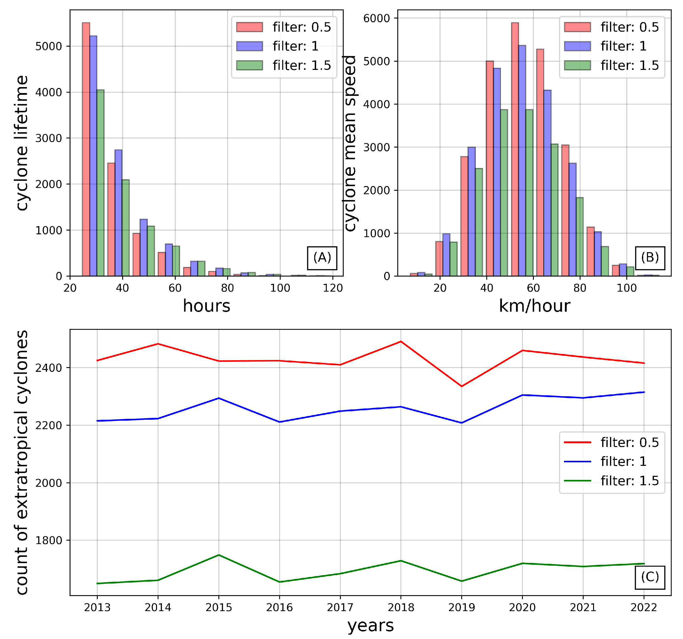
3.1. Sensitivity to the Smoothing Parameter for the Relative Vorticity Field

Figure 4A shows the mean sea level (contours) and relative vorticity field (shading) obtained directly from ERA5 for 1 July 2020, 12 UTC, when an intense extratropical cyclone was near the coast of Uruguay and southern Brazil (35° S/46° W) and another weak cyclone was positioned at 50° S and 48° W. Using standard deviation of Gaussian filter of 0.5 to the same time frame (Figure 4B), intense characteristic of coastal cyclone and weak characteristic of the southeast cyclone are preserved. However, tests of sigma equal to 1 (Figure 4C) and 3 (Figure 4D) over-smoothed the relative vorticity field, to the extent of nullifying the weak event or reducing its area. A test of sigma equal to 5 underestimates the number of cyclones for 2020 (not shown) giving unrealistic results.
According to analysis of the relative vorticity field of this known event, it can be seen that weak events are detected just in low level of smoothing, then a more detailed study of the extratropical cyclone features is shown just to 0.5, 1.0 and 1.5 degree of smoothing, applied to 10 years in Figure 5. As expected, the number of events depends on the filtering strength, with more events using lower degree of smoothing. Figure 5A shows that there are more events of less than two days and Figure 5B shows that the mean speed of the events are between 40 km/h and 60 km/h using the three levels of smoothing. These are expected features of cyclones in Southern Hemisphere. The mean count of extratropical cyclones is 2430, 2258 and 1693 using 0.5, 1.0 and 1.5 respectively. Thus, the supression of events was on average 25%, comparing smoothing level from 1.0 to 1.5, and 7% comparing 0.5 to 1.0. For the following steps, we used a smoothing parameter of 0.5.

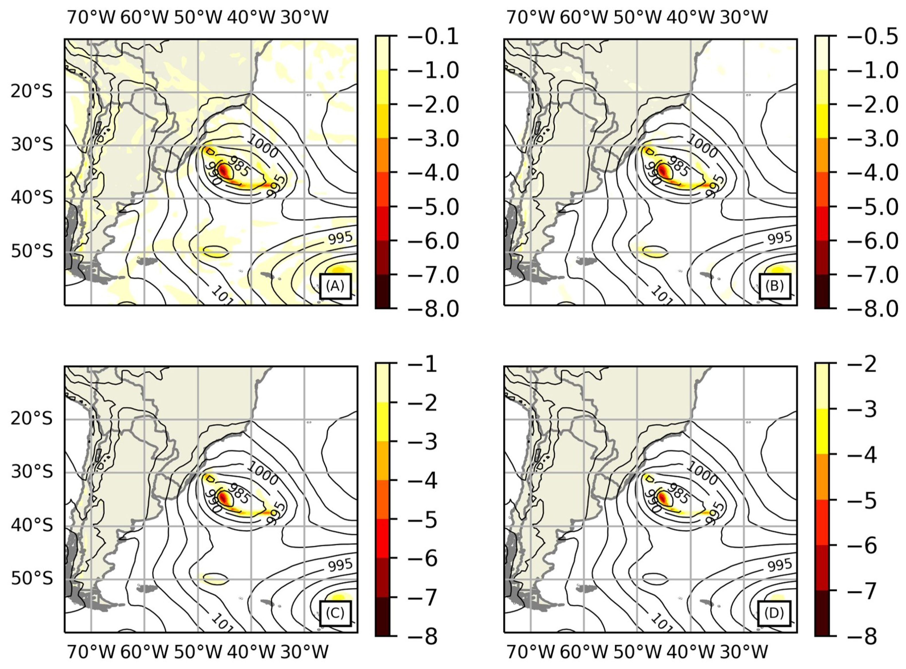
3.2. Sensitivity to Threshold of Relative Vorticity

The choice of the threshold of relative vorticity will calibrate the number of possible cyclone centers and remove signals that are not related to these systems. Figure 6 shows the relative vorticity field from ERA5/ECMWF on 1 July 2020, 12 UTC, with the standard deviation of Gaussian filter of 0.5, for four different thresholds of relative vorticity. Figure 6A shows a noisy field with a threshold of −10−5 s−1. A threshold of −0.5 × 10⁻⁴ s−1 generates a spurious signal mainly at the Andes (Figure 6B). On the other hand, the threshold of 2 × 10⁻⁴ s−1 (Figure 6D) cannot identify the cyclone centers in the region. Then, from the visual analysis of the relative vorticity field, we conclude that a good threshold to identify the events and suppress the spurious signals in our tests is 10−4 s−1 (Figure 6C).

3.3. Sensitivity to the Minimum Area of Relative Vorticity under the Threshold

Figure 7 presents the mean monthly cyclone centers detected between 2013 and 2022 using 0.5 of filter parameter, threshold of relative vorticity of 10−4 s−1 and with different thresholds of minimum area of relative vorticity labels. As expected, the number of cyclone centers per day depends on the choice of the minimum area size. This criterion should be neither so strict as to remove real small cyclones, nor so lenient as to include spurious cyclones. Furthermore, there is an expectation that more events will take place in the winter than in the summer because the large-scale temperature gradients are higher in the winter [3]. Using a minimum area of less than 9 points (not shown) yields an unrealistic number of cyclones (more than 1000 per month). It can be an indication that persistent signals are counted as different cyclone events, like those generated by orography. However, Figure 7 shows minimum area tests of 9, 12, 15 and 18 points and the expected increase in the number of cyclones in winter is obtained. Moreover, correlation of monthly number of cyclones between the 9 and 12 tests are 0.983, between 12 and 15 tests are 0.987 and between 15 and 18 are 0.985, suggesting that the results converge around test of minimum area equal to 15.
Figure 8 shows the frequency distribution of cyclone lifetime (A), frequency distribution of cyclone mean speed (B) and the time series of total annual number of extratropical cyclones between 2013 and 2022 (C). Although the number of cyclones detected using the different tests are clearly dependent on the choice of the minimum area criterion, cyclone lifetime and mean speed distribution are similar using the four tests. Table 2 shows the mean lifetime and standard deviation in hours and the mean speed mean and standard deviation for the four tests and they have no significant changes on the results. This means that these characteristics of cyclones are not sensitive to the area criteria within this range of values. For the rest of the study, we selected the 15 minimum area criteria as a good choice.

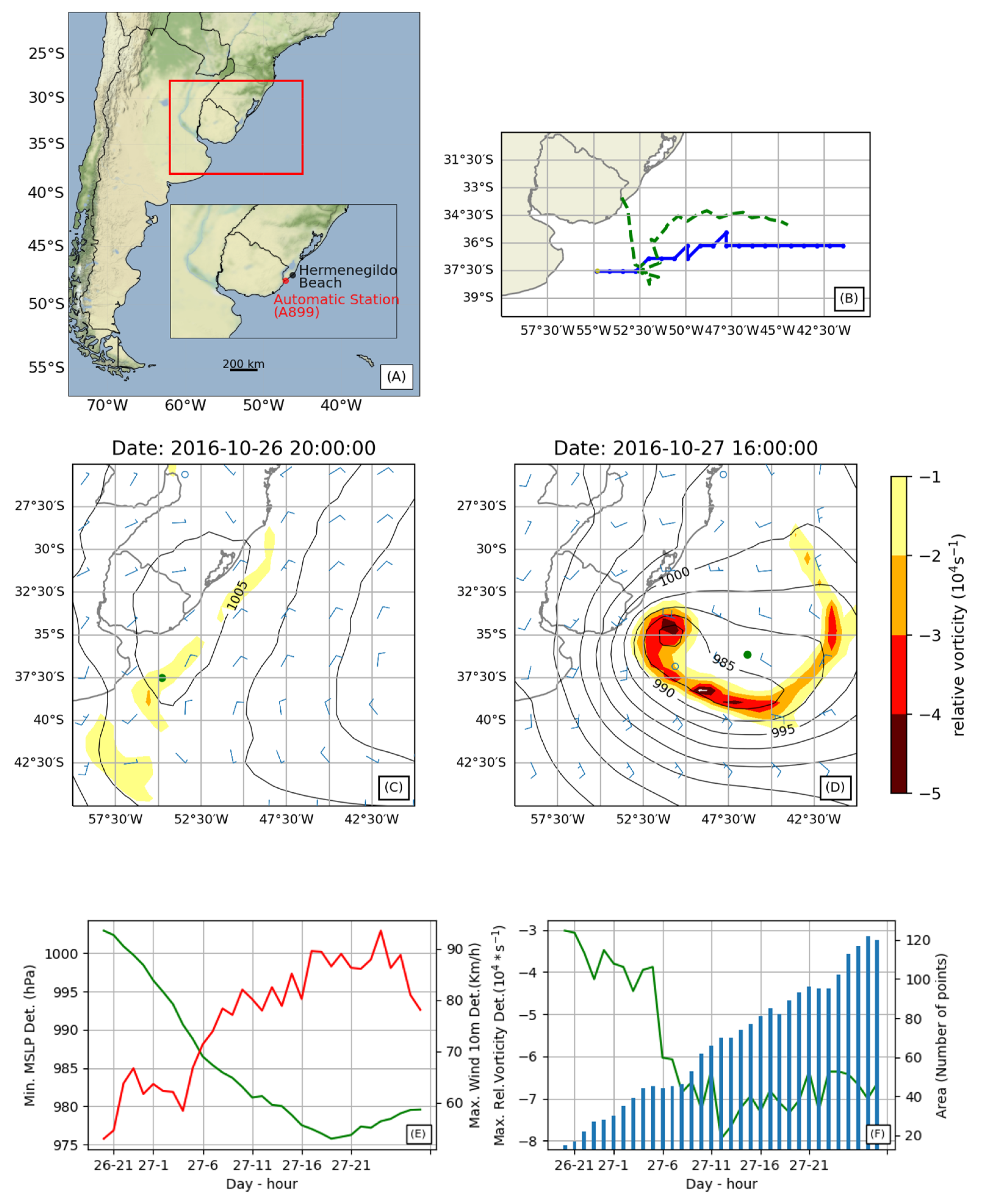
3.4. First Case Study: Extratropical Cyclone of 26–28 October 2016

An intense extratropical event in southern Brazil was documented by Albuquerque et al. [40] and Oliveira et al. [41], with impacts at Hermenegildo beach (33.7° S, 53.4° W, Figure 9A). It was an event of high wave energy, with significant shifts in coastal morphology. The automatic station of Santa Vitoria do Palmar (identified by A899), at 33.74° S/53.37° W (Figure 9A), recorded a maximum wind gust of 111.2 Km/h at 17 UTC of 27 October 2016 and a minimum mean sea level pressure of 997.4 hPa at 15 UTC and 16 UTC of 27 October 2016. The cyclone started to develop on 26 October, with lower mean sea level pressure over Uruguay and southern Brazil. Figure 9B shows the storm track identified by the algorithm (blue line) and identified by a visual inspection of the pressure field (green line). The evolution of the cyclone track from the algorithm agrees relatively well with that from the visual detection. Figure 9C,D show the similarity of the visual field inspection and the algorithm results (green point) and the location of the extratropical cyclone at the initial frame (20 UTC 27 October) and during the more intense stage (16 UTC on 27 October) respectively. Figure 9E,F show the evolution of cyclone intensity by the maximum 10-m winds, minimum mean sea level pressure, maximum relative vorticity detection and the size of vorticity above the threshold at each time frame. All the parameters show the intense period between 12 UTC on 27 October and 03 UTC on 28 October. The last time frame has strong winds, low mean sea level pressure and intense relative vorticity, which may be associated with a loss of the cyclolysis process. These results suggest that our algorithm had the best accuracy at the initial stage and during the intense period of the cyclone for the case study.

3.5. Second Case Study: Extratropical Cyclone of 15–17 August 2020

The second case study has the important feature of merging with another low-pressure center. When two or more neighbouring cyclones merge or split, the recognition of the cyclone trajectory becomes more difficult [42]. There is an improvement in recognizing merging or splitting extratropical cyclones by using techniques such as connected-component label (e.g., [10,12,26,42]). Figure 10A shows the storm track identified by the algorithm (blue line) and that identified by a visual inspection (green line), using sea level pressure field. Both tracks converge over all stages of the cyclone lifecycle. The extratropical cyclone developed over the southwest Atlantic at 20 UTC on 15 August 2020 (Figure 10B). Figure 10C shows the event in the more intense stage, with a maximum relative vorticity of −8.6 −10−4 s−1. Along the southeastward displacement, it started to merge at 00 UTC on 17 August 2020. Figure 10D shows the event on the merged stage.
Figure 10E,F present the evolution of minimum sea level pressure, maximum 10-m winds, maximum relative vorticity at 850 hPa and total area above the threshold over the cyclone time frames. A minimum mean sea level pressure and a maximum area above the threshold occurred during the last hours of 16 August. However, the maximum winds and more intense relative vorticity was during the early hours of the event. This can be a consequence of the merging process just before the weakening that is observed during cyclolysis. In the subsequent time frame, the algorithm maximum displacement part promoted the end of the event. Possibly part of the decay process of the event was not included by the program, due to the increase in area within the threshold, which displaces the calculated center of mass, making the dissolution phase shorter. These two events highlight the ability of the method to track the cyclogenesis process and the more intense stage of the events and a possible suppression of part of the cyclolysis stage.

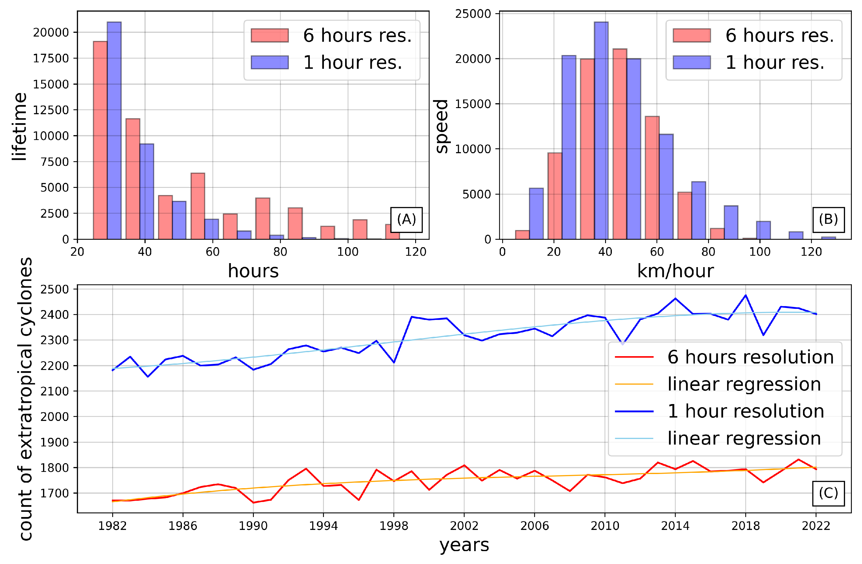
3.6. Temporal Resolution

We expect that the finer the temporal resolution, the better the tracking process because the search in the following time step is done within a shorter time gap, and a shorter radius of searching if the propagation speed does not change [16]. Another implication of using higher time resolution data is that the cyclones are weaker on the average, because weaker systems with shorter tracks are not identified in coarser time resolution data [21]. However, Crawford et al. [23] examined the sensitivity of cyclone detection and tracking for the Northern Hemisphere and showed that refining beyond 3 h does not necessarily lead to more accurate detection and tracking, using the algorithm explained by Crawford and Serreze [22] applied to finer temporal resolution dataset.
In addition to this, most climatology are constructed based on 6-hourly atmospheric fields. Gramcianinov [30] compared the 6-hourly and 1-hourly tracking using the same tracking method and thresholds. The results showed a higher genesis density in Uruguay and a smaller density in southern Brazil, using 1-hourly data. According to the authors, this difference can be associated with the identification of the cyclonic systems at earlier stages of development using 1-hourly data.
Our study compares the cyclone tracking performance using 6-hourly and 1-hourly datasets. Figure 11 shows the frequency distribution of cyclone lifetime, cyclone mean speed and the count of extratropical cyclones per year from 1982 to 2022, with 1-hourly and 6-hourly temporal resolution. Crawford et al. [43] detached that changing from 6-hourly to 1-hourly resolution shorter events are more inclined to late detection or early termination and explained that this leads to a grow of short-lived events. The same influence was observed in ours results, that is more events of less than two days using 1-hourly resolution. In terms of mean speed, although the mean values are similar, the frequency distribution is more dispersed using 1-hourly resolution, with a standard deviation of 21.2 km/h to 1-hourly and 15.3 km/h to 6-hourly resolution. The time series of total annual number of extratropical cyclones for the two resolutions, applied to 41 years (Figure 11C) show an increasing tendency. The coefficient of determination is of 0.56 and 0.77 for 6-hourly and 1-hourly resolution, respectively.
Violin plot of extratropical cyclone tracking in Southern Hemisphere for the period of 1982–2022 (Figure 12A) highlights that 1-hourly temporal resolutions has more events per year than 6-hourly resolution, with an average of 2314 for the 1-hourly dataset and 1750 for the 6-hourly dataset.
Considering the period of 1982 to 2022, the duration of the events using 1-hourly and 6-hourly datasets has analogous difference to the frequency distribution of lifetime, with an average of 24 h from the former and 49 h for the latter (Figure 12B). One explanation to this difference could be a premature termination of tracks and/or split of two tracks in situations that would be continued if analysed manually by a meteorologist. These issues can be addressed in a future improvement of the program. Heading of Figure 12C, track length in km tends to be shorter using the finer temporal resolution dataset, because the search of the next frame has a shorter time gap, and this implies more details along the cyclone track, with more events of short lifetime and short distance traveled included in the group of events. The track distance averages from 1355 km using the 1-hourly dataset to 2224 km using 6-hourly dataset. The third quartile also shows a difference, with 1628 km and 2917 km using 1-hourly and 6-hourly dataset resolution, respectively.
The evaluation of cyclone speed (Figure 12D) shows similar average values using the 6-hourly dataset comparing to those obtained by IMILAST intercomparison project. However, the average speed 56 km/h using the 1-hourly dataset is slightly higher than that from the 6-hourly dataset (46 km/h) and IMILAST intercomparison project. This can be explained by the inclusion of faster cases, with finer temporal resolution and the more disperse distribution shown in Figure 11B.
Focusing on the intensity of the events, Figure 12E shows the relative vorticity minimum at 850 hPa, identified using the two temporal resolutions. The averages are −4.4 × 10⁻⁴ s−1 and −4.3 × 10⁻⁴ s−1 for the 1-hourly and 6-hourly datasets, respectively. As expected, using the 1-hourly resolution, the algorithm is more efficient in finding the most intense events, indicated by the elongated range of values in the violin plot. In terms of the average of the area with relative vorticity above the threshold (Figure 12F), the two temporal resolutions are similar, 106 and 95 for the 1-hourly and 6-hourly dataset, respectively. When using the finer resolution, the algorithm captures slightly larger areas.

3.7. Extratropical Cyclone Climatology

Generally, studies using different methodologies of detecting and tracking of extratropical cyclones present the number of cyclone centers, either by month or season, and per unit area over a hemisphere. This is called system density by Simmonds and Keay [24]. When these results are presented as a percentage of the total time, it is usually called cyclone frequency or cyclone density [27]. Most of the previous studies use different 6-hourly reanalysis datasets. To determine the robust features among the different methodologies, the IMILAST project compiled climatologies of cyclone frequency over the same period (20-yr period), with the same time resolution (6 hourly), and the same dataset (ERA-Interim/ECMWF dataset, with 1.5° spatial resolution), with the same minimum lifetime of 24 h [27], for both hemispheres. Here, we compare the results obtained from our algorithm with those from the IMILAST project and other studies, taking into consideration that our study uses a different dataset, with higher temporal and spatial resolution, for a longer period. So, we intend to present the similarities and differences with these assumptions in mind.
Figure 13 shows the mean number of cyclogenesis per month, with a cap area of 106 km2 in the Southern Hemisphere for the four seasons. It is evident that the greatest number of cyclogenesis occurs along the 70° S–50° S latitude band, which agrees with Simmonds and Keay [24]. Consistent with previous studies and as expected, the frequency and spatial extent of cyclogenesis are higher during winter. Our methodology also reproduces the absence of cyclogenesis west of the Andes and an intensification of cyclogenesis along the southeastern coast of South America [44,45]. As the perturbation crosses the Andes at middle latitudes, the lower-level perturbation advances following the orography and propagates on the lee side of the Andes, detached from the upper-level perturbation and suppressing the instability. Approaching the southeastern coast of South America, the perturbation encounters a more favorable baroclinic structure, promoting cyclogenesis. The strong region of cyclogenesis observed in the coastal area of Antarctica was also observed by Treut and Kalnay [46], Murray and Simmonds [7],Hodges [33], Simmonds and Keay [24], Hoskings and Hodges [47] and Valsangkar et al. [48].

4. Discussion and Conclusions

In this article, we presented an algorithm to detect and track extratropical cyclones, studying the choice of parameters for the ERA5 reanalysis, in the Southern Hemisphere. To identify cyclonic centers, we use relative vorticity at 850 hPa and connected-component labeling, which tracks cyclones as areas rather than local minimums. We tested the use of three degrees of filtering smoothing of gaussian filter to determine the ideal level of filtering for the best detection of cyclones. Also, we showed an example of relative vorticity field at 850 hPa, using different thresholds for relative vorticity and tested four different values of minimum area criteria. With these analyses, we adjusted within the algorithm to improve its performance. We use standard deviation of the gaussian filter of 0.5 grid points, threshold of relative vorticity of −10−4 s−1, and area criteria of 15 pixels. The maximum displacement in one hour was fixed to 150 km.
The two case studies presented here highlighted the good performance to detect cyclogenesis and the more intense periods of the cyclones and identify cyclones that merge/split along their lifetime. However, the position of the cyclone center during the cyclolysis can be inaccurate, because of the increase in the area within the threshold, possible suppressing part of the dissipation process, as shown by the second case study. Despite these findings, we believe that the algorithm is useful for studying extratropical cyclones and exploring the different characteristics of the events.
Comparing the results using 1-hourly and 6-hourly temporal resolution, we find a greater average number of events per year using 1-hourly temporal resolution. This can be explained by the greater precision in identifying the time frame of cyclogenesis and cyclolysis with a finer resolution, and by the inclusion of some shorter events that would have been removed by the minimum lifetime threshold. Using 41 years of data, the annual count of extratropical cyclones of Southern Hemisphere displayed a slowly increasing trend in both temporal resolution. The duration of the cyclones of around 2 days is slightly larger using 6-hourly temporal resolutions, but it is in agreement with Neu [16], which compares various methodologies using 6-hourly resolution dataset. The distance traveled by the cyclones was a little longer using the 6-h temporal resolution due to the removal of shorter cases. The cyclones captured by 1-h temporal resolution are in average faster than those by the 6-h temporal resolution. Our 6-h temporal resolution results agreed with IMILAST in term of average speed, mainly ranging from 20 km/h to 60 km/h.
The spatial distribution of cyclogenesis frequency from our algorithm is very similar to those from other studies, in particular with regard to the most favorable areas of development of extratropical cyclones. In general, the number of events is consistent with previous studies, although there is no consensus on this among the various methods, as shown by the IMILAST project. In terms of areas of suppression and intensification of cyclogenesis in the Southern Hemisphere, our results are consistent with previous studies. Further improvements to the algorithm can be made, such as including different parameter thresholds at different altitude levels. The algorithm was implemented in Python, and its source code is freely available from the authors upon request.
Future research using the methodology developed in this study includes understanding the interannual variability of the characteristics of extratropical cyclones along the southeastern coast of South America and potential links to extreme events of ocean temperature, known as marine heat waves.

Author Contributions

Conceptualization, C.K.P.R.; methodology, C.K.P.R.; software, C.K.P.R.; validation, C.K.P.R.; formal analysis, C.K.P.R. and J.P.M.; investigation, C.K.P.R.; writing—original draft preparation, C.K.P.R. and J.P.M.; writing—review and editing, J.P.M., M.M.M., R.R. and J.L.L.d.A.; supervision, J.M.B.S.; project administration, C.K.P.R. All authors have read and agreed to the published version of the manuscript.

Funding

National Council for Scientific and Technological Development (CNPq), projects n° 406769/2021-4 and 406763/2022-4.

Institutional Review Board Statement

Not applicable.

Informed Consent Statement

Not applicable.

Data Availability Statement

The ERA5/ECMWF reanalysis data is accessible at https://cds.climate.copernicus.eu/cdsapp#!/dataset/reanalysis-era5-single-level?tab=overview accessed on 23 May 2023 and the identification and tracking program is freely available upon request (carina.padilha@gmail.com).

Acknowledgments

We are also grateful to the National Council for Scientific and Technological Development (CNPq) for projects funding (n° 406769/2021-4 and 406763/2022-4). We thank the resources provided by CAPES to support the Graduate Program in Oceanology.

Conflicts of Interest

The authors declare no conflict of interest.

References

  1. Wallace, J.M.; Hobbs, P.V. The General Circulation. In An Introductory Survey, 2nd ed.; Elsevier: Amsterdam, The Netherlands; Academic Press: Boston, MA, USA, 2006; pp. 412–450. [Google Scholar]
  2. Peixoto, J.P.; Oort, A.H. Phisics of Climate; American Institute of Phisics: College Park, ML, USA, 1992; 520p. [Google Scholar]
  3. Ulbrich, U.; Leckebusch, G.C.; Pinto, J.G. Extra-tropical cyclones in the present and future climate: A review. Theor. Appl. Climatol. 2009, 96, 117–131. [Google Scholar] [CrossRef]
  4. Catto, J.L.; Ackerley, D.; Booth, J.F.; Champion, A.J.; Colle, B.A.; Pfahl, S.; Pinto, J.G.; Quinting, J.F.; Seiler, S. The Future of Midlatitude Cyclones. Curr. Clim. Chang. Rep. 2019, 5, 407–420. [Google Scholar] [CrossRef]
  5. Sinclair, V.A.; Rantanen, M.; Haapanala, P.; Räisänen, J.; Järvinen, H. The characteristics and structure of extra-tropical cyclones in a warmer climate. Weather Clim. Dyn. 2020, 1, 1–25. [Google Scholar] [CrossRef]
  6. Lambert, S.J. A cyclone climatology of the Canadian climate centre general circulation. J. Clim. 1988, 1, 109–115. [Google Scholar] [CrossRef]
  7. Murray, R.J.; Simmonds, I. A numerical scheme for tracking cyclone centres from digital data. Part I: Development and operation of the scheme. Aust. Meteorol. Mag. 1991, 39, 155–166. [Google Scholar]
  8. Lionello, P.; Dalan, F.; Elvini, E. Cyclones in the Mediterranean region: The present and the doubled CO2 climate scenarios. Clim. Res. 2002, 22, 147–159. [Google Scholar] [CrossRef]
  9. Rudeva, I.; Gulev, S.K. Climatology of cyclone size characteristics and their changes during the cyclone life cycle. Mon. Weather Rev. 2007, 135, 2568–2587. [Google Scholar] [CrossRef]
  10. Hanley, J.; Caballero, R. Objective identification and tracking of multicentre cyclones in the ERA-Interim reanalysis dataset. Q. J. R. Meteorol. Soc. 2012, 138, 612–625. [Google Scholar] [CrossRef]
  11. Sinclair, M.R. An objective cyclone climatology for the Southern Hemisphere. Mon. Weather Rev. 1994, 122, 2239–2256. [Google Scholar] [CrossRef]
  12. Inatsu, M. The neighbor enclosed area tracking algorithm for extratropical wintertime cyclones. Atmos. Sci. Lett. 2009, 10, 267–272. [Google Scholar] [CrossRef]
  13. Hodges, K.I. A general method for tracking analysis and its application to meteorological data. Mon. Weather Rev. 1994, 12, 2573–2586. [Google Scholar] [CrossRef]
  14. Reboita, M.S.; da Rocha, R.P.; de Souza, M.R.; Llopart, M. Extratropical cyclones over the southwestern South Atlantic Ocean: HadGEM2-ES and RegCM4 projections. Int. J. Climatol. 2018, 38, 2866–2879. [Google Scholar] [CrossRef]
  15. Hodges, K.I.; Hoskins, B.J.; Boyle, J. A Comparison of Recent Reanalysis Datasets Using Objective Feature Tracking: Storm Tracks and Tropical Easterly Waves. Mon. Weather Rev. 2003, 131, 2012–2037. [Google Scholar] [CrossRef]
  16. Blender, R.; Shubert, M. Cyclone Tracking in Different Spatial and Temporal Resolutions. Mon. Weather Rev. 2000, 128, 377–384. [Google Scholar] [CrossRef]
  17. Trigo, I.F. Climatology and interannual variability of storm-tracks in the Euro-Atlantic sector: A comparison between ERA-40 and NCEP/NCAR reanalyses. Clim. Dyn. 2006, 26, 127–143. [Google Scholar] [CrossRef]
  18. Flaounas, E.; Kotroni, V.; Lagouvardos, K.; Flaounas, I. CycloTRACK (v1.0)-tracking winter extratropical cyclones based on relative vorticity: Sensitivity to data filtering and other relevant parameters. Geosci. Model Dev. 2014, 7, 1841–1853. [Google Scholar] [CrossRef]
  19. Lim, E.P.; Simmonds, I. Southern hemisphere winter extratropical cyclone characteristics and vertical organization ob-served with the ERA-40 data in 1979–2001. J. Clim. 2007, 20, 2675–2690. [Google Scholar] [CrossRef]
  20. Wang, X.L.; Swail, V.R.; Zwiers, F.W. Climatology and Changes of Extratropical Cyclone Activity: Comparison of ERA-40 with NCEP-NCAR Reanalysis for 1958–2001. J. Clim. 2006, 19, 3145–3166. [Google Scholar] [CrossRef]
  21. Pinto, J.G.; Spangehl, T.; Ulbrich, U.; Speth, P. Sensitivities of a cyclone detection and tracking algorithm: Individual tracks and climatology. Meteorol. Z. 2005, 14, 823–838. [Google Scholar] [CrossRef]
  22. Crawford, A.D.; Serreze, M.C. Does the Summer Arctic Frontal Zone Influence Arctic Ocean Cyclone Activity? J. Clim. 2016, 29, 4977–4993. [Google Scholar] [CrossRef]
  23. Crawford, A.D.; Schreiber, E.A.P.; Sommer, N.; Serreze, M.C.; Stroeve, J.C.; Barber, D.G. Sensitivity of Northern Hemisphere Cyclone Detection and Tracking Results to Fine Spatial and Temporal Resolution Using ERA5. Mon. Weather Rev. 2021, 149, 2581–2598. [Google Scholar] [CrossRef]
  24. Simmonds, I.; Keay, K. Variability of Southern Hemisphere Extratropical Cyclone Behavior, 1958-97. J. Clim. 2000, 13, 550–561. [Google Scholar] [CrossRef]
  25. Reboita, M.S.; da Rocha, R.P.; Ambrizzi, T.; Sugahara, S. South Atlantic Ocean cyclogenesis climatology simulated by regional climate model (RegCM3). Clim. Dyn. 2010, 35, 1331–1347. [Google Scholar] [CrossRef]
  26. Hewson, T.D.; Titley, H.A. Objective identification, typing and tracking of the complete life-cycles of cyclonic features at high spatial resolution. Meteorol. Appl. 2009, 17, 355–381. [Google Scholar] [CrossRef]
  27. Neu, U.; Akperov, M.G.; Bellenbaum, N.; Benestad, R.; Blender, R.; Caballero, R.; Cocozza, A.; Dacre, H.F.; Feng, Y.; Fraedrich, K.; et al. Imilast: A community effort to inter-compare extratropical cyclone detection and tracking algorithms. Bull. Am. Meteorol. Soc. 2013, 94, 529–547. [Google Scholar] [CrossRef]
  28. Raible, C.C.; Della-Marta, P.M.; Schwierz, C.; Wernli, H.; Blender, R. Northern Hemisphere extratropical cyclones: A comparison of detection and tracking methods and different reanalyses. Mon. Weather Rev. 2009, 136, 880–897. [Google Scholar] [CrossRef]
  29. Reale, M.; Margarida, L.R.; Liberato, L.R.; Lionello, P.; Pinto, J.G.; Salon, S.; Ulbrich, S. A Global Climatology of Explosive Cyclones using a Multi-Tracking Approach. Tellus Dyn. Meteorol. Oceanogr. 2019, 71, 1611340. [Google Scholar] [CrossRef]
  30. Gramcianinov, C.B.; Campos, R.M.; Camargo, R.; Hodges, K.I.; Soares, C.G.; da Silva Dias, P.L. Analysis of Atlantic extratropical storm tracks characteristics in 41 years of ERA5 and CFSR/CFSv2 databases. Ocean. Eng. 2020, 216, 108111. [Google Scholar] [CrossRef]
  31. Hersbach, H.; Bell, B.; Berrisford, P.; Hirahara, S.; Horányi, A.; Muñoz-Sabater, J.; Nicolas, J.; Peubey, C.; Radu, R.; Schepers, D.; et al. The ERA5 global reanalysis. Q. J. R. Meteorol. Soc. 2020, 146, 1999–2049. [Google Scholar] [CrossRef]
  32. Holton, J.R. Introduction to Dynamic Meteorology, 4th ed.; Elsevier: Amsterdam, The Netherlands, 2004; p. 535. [Google Scholar]
  33. Hodges, K.I. Feature tracking on the unit sphere. Mon. Weather Rev. 1995, 123, 3458–3465. [Google Scholar] [CrossRef]
  34. Hoskins, B.J.; Hodges, K.I. New Perspectives on the Northern Hemisphere winter storm tracks. J. Atmos. Sci. 2002, 59, 1041–1061. [Google Scholar] [CrossRef]
  35. Satake, Y.; Inatsu, M.; Mori, M.; Hasegawa, A. Tropical cyclone tracking using a neighbor enclosed area tracking algorithm. Mon. Weather Rev. 2013, 141, 3539–3555. [Google Scholar] [CrossRef]
  36. Gonzales, R.C.; Woods, R.E.; Prentice Hall, P. Digital Image Processing, 3rd ed.; Pearson International Edition; Pearson Education: London, UK, 1992. [Google Scholar]
  37. Samet, H. Applications of Special Data Structures: Computer Graphics, Image Processing and GIS; Addison-Wesley: Boston, MA, USA, 1989; 507p. [Google Scholar]
  38. Inatsu, M.; Amada, S. Dynamics and geometry of extratropical cyclones in the upper troposphere by a neighbor enclosed area tracking algorithm. J. Clim. 2013, 26, 8641–8653. [Google Scholar] [CrossRef]
  39. Bai, L.; Breen, D. Calculating Center of Mass in an Unbounded 2D Environment. J. Graph. Tools 2008, 13, 53–60. [Google Scholar] [CrossRef]
  40. Albuquerque, M.D.G.; Leal Alves, D.C.; Espinoza, J.M.D.A.; Oliveira, U.R.; Simões, R.S. Determining Shoreline Res-ponse to Meteo-oceanographic Events Using Remote Sensing and Unmanned Aerial Vehicle (UAV): Case Study in Southern Brazil. J. Coast. Res. 2018, 85, 766–770. [Google Scholar] [CrossRef]
  41. Oliveira, U.R.; Simões, R.S.; Calliari, L.J. Dunes erosion under an extreme high wave energy event on the central and southern coast of Rio Grande do Sul state, Brazil. Rev. Bras. Geomorfol. 2019, 20, 137–158. [Google Scholar] [CrossRef]
  42. Lu, C. A modified algorithm for identifying and tracking extratropical cyclones. Adv. Atmos. Sci. 2017, 34, 909–924. [Google Scholar] [CrossRef]
  43. Crawford, A.D.; Alley, E.E.; Cooke, A.M.; Serreze, M.C. Synoptic climatology of rain-on-snow events in Alaska. Mon. Weather Rev. 2020, 148, 1275–1295. [Google Scholar] [CrossRef]
  44. Gan, M.A.; Rao, V.B. The influence of the Andes Cordillera on transient disturbances. Mon. Weather Rev. 1994, 122, 1141–1157. [Google Scholar] [CrossRef]
  45. Vera, C.S.; Vigliarolo, P.K.; Berbry, E.H. Cold season synoptic-scale waves over subtropical South America. Mon. Weather Rev. 2002, 130, 684–699. [Google Scholar] [CrossRef]
  46. Treut, H.L.; Kalnay, E. Comparison of observed and simulated cyclone frequency distribution as determined by an objective method. Atmósfera 1990, 3, 57–71. [Google Scholar]
  47. Hoskins, B.J.; Hodges, K.I. A new perspective on Southern Hemisphere storm tracks. J. Clim. 2005, 18, 4108–4129. [Google Scholar] [CrossRef]
  48. Valsangkar, A.; Monteiro, J.M.; Narayanan, V.; Hotz, I.; Natarajan, V. An Exploratory Framework for Cyclone Identification and Tracking. IEEE Trans. Vis. Comput. Graph. 2019, 10, 1–14. [Google Scholar]
Figure 1. Example of points center of mass of areas that match the relative vorticity threshold-sequence of hourly data.
Atmosphere 15 00230 g001
Figure 2. Mean sea level pressure and relative vorticity at 850 hPa under −10−4 s−1, on 27 October 2016, 06 UTC. The green square is the “effective area” to search for the more intense characteristics of the cyclone. The yellow point is the center of mass identified by the algorithm and the blue line and points are the following time frames of the event.
Atmosphere 15 00230 g002
Figure 3. Flowchart of the detection algorithm of extratropical cyclones proposed in this study.
Atmosphere 15 00230 g003
Figure 4. Mean sea level pressure and relative vorticity at 850 hPa under −10−4 s−1, on 1 July 2020, 12 UTC. (A) raw data and with different standard deviations of the Gaussian filter: (B) 0.5, (C) 1.0 and (D) 3.0.
Atmosphere 15 00230 g004
Figure 5. Study of the features of cyclones for the three sensitivity tests of filter degree, computed from 2013 to 2022: (A) Frequency distribution of cyclone lifetime, (B) frequency distribution of cyclone mean speed and (C) time series of total annual number of extratropical cyclones.
Atmosphere 15 00230 g005
Figure 6. Mean sea level pressure (contours) and relative vorticity at 850 hPa (shading) with thresholds of: (A) −10−5 s−1; (B) −0.5 × 10⁻⁴ s−1; (C) −10−4 s−1 and (D) −2 × 10⁻⁴ s−1, on 1 July 2020, 12 UTC, using a Gaussian filter parameter of 0.5.
Atmosphere 15 00230 g006
Figure 7. Mean Cyclone centers per month detected between 2013 and 2022, using a Gaussian filter parameter of 0.5, a threshold of relative vorticity of −10−4 s−1 and different sets of minimum area (number of pixels).
Atmosphere 15 00230 g007
Figure 8. Study of the features of cyclones for the four sensitivity tests of area criterion, computed between 2013 and 2022: (A) Frequency distribution of cyclone lifecicle, (B) frequency distribution of cyclone mean speed and (C) time series of total annual number of extratropical cyclones.
Atmosphere 15 00230 g008
Figure 9. Extratropical cyclone during 26 to 28 October 2016. (A) Location of Hermenegildo Beach and automatic station of Chui (A899). (B) Cyclone track from 26 October 2016, 20 UTC to 28 October 2016, 6 UTC obtained from the program (blue line) and visual inspection (green line). (C) Mean sea level pressure and relative vorticity at 850 hPa, on 26 October 2016, 20 UTC, the green point is the position obtained from the algorithm. (D) Same as (C) except for: 27 October 2016, 16 UTC. (E) Minimum mean sea level pressure (green line) and maximum 10-m wind (red line) detected by the algorithm during the event. (F) Minimum relative vorticity (green line) and total area under the threshold (blue histograms) detected by the algorithm during the event.
Atmosphere 15 00230 g009
Figure 10. Extratropical Cyclone of 15 to 17 August 2020. (A) Cyclone track from 15 August 2020, 20 UTC to 17 August 2020, 06 UTC, obtained from the algorithm (blue line) and from visual inspection (green line). (B) Mean sea level pressure and relative vorticity at 850 hPa, 15 August 2020, 20 UTC, the green point is the position obtained from the algorithm. (C) Same as (B) except for: 16 August 2020, 06 UTC. (D) Same as (B) except for: 17 August 2020, 02 UTC. (E) Minimum mean sea level pressure (green line) and maximum 10-m wind (red line) detected by the algorithm during the event. (F) Minimum relative vorticity (green line) and total area under the threshold (blue bars) detected by the algorithm during the event.
Atmosphere 15 00230 g010
Figure 11. Study of the features of cyclones in the Southern Hemisphere using 1-hourly (blue) and 6-hourly (orange) temporal resolutions, for the period of 1982–2021: (A) Frequency distribution of cyclone lifecicle, (B) frequency distribution of cyclone mean speed and (C) time series of total annual number of extratropical cyclones.
Atmosphere 15 00230 g011
Figure 12. Violin plot of extratropical cyclones tracking in the Southern Hemisphere using 1-hourly (blue) and 6-hourly (orange) temporal resolutions, for the period of 1982–2022. (A) Events per year. (B) Duration in hours. (C) Track length in km. (D) Average speed in km/h. (E) Minimum relative vorticity of events in s−1. (F) Maximum area with relative vorticity under the threshold.
Atmosphere 15 00230 g012
Figure 13. The average number of cyclogenesis per month in the Southern Hemisphere, with a cap area of 106 km2. (A) Winter: June, July and August, (B) Summer: December, January and February, (C) Spring: September, October and November, (D) Autumn: March, April and May.
Atmosphere 15 00230 g013
Table 1. Relevant extratropical ciclone detecting and tracking methods.
ReferencesVariable Used to IdentifyMain Characteristics
Blender and Scubert, 2000 [16]; Trigo, 2006 [17].local minimum of the geopotential height of the 1000-hPa surfacenearest-neighbor search method
Crawford and Serreze, 2016 [22]; Crawford et al., 2021 [23]; Hanley and Caballero, 2012 [10]; Lionello et al., 2002 [8]Minimum mean sea level pressurenearest-neighbor search method
Murray and Simmonds, 1991 [7]; Simmonds and Keay, 2000 [24], Lim and Simmonds, 2007 [19]; Pinto et al., 2005 [21]; Rudeva and Gulev, 2007 [9].Minimum mean sea level pressureestimate the subsequent displacement and pressure change
Reboita et al., 2010 [25]; Reboita et al., 2017 [14]relative vorticity of the 925 hPa surfacenearest-neighbor search method
Inatsu, 2009 [12]relative vorticity of the 850 hPa surfacearea under a threshold
Flauonas, 2014 [18]relative vorticity of the 850 hPa surfacemost natural evolution of relative vorticity field
Hewson and Titley, 2010 [26]mean sea level pressure and relative vorticitygraphical processing
Table 2. Statistics information of lifetime and mean speed of detected cyclones using different minimum area tests.
Minimum Area TestLifetime MeanLifetime Standard DeviationMean Speed MeanMean Speed Standard Deviation
924.912.656.416.5
1224.812.256.316.4
1524.612.056.316.2
1824.411.756.316.1
Disclaimer/Publisher’s Note: The statements, opinions and data contained in all publications are solely those of the individual author(s) and contributor(s) and not of MDPI and/or the editor(s). MDPI and/or the editor(s) disclaim responsibility for any injury to people or property resulting from any ideas, methods, instructions or products referred to in the content.

