Article

Detecting Relationship between the North–South Difference in Extreme Precipitation and Solar Cycle in China

1
Chinese Academy of Meteorological Sciences, China Meteorological Administration, Beijing 100081, China
2
Key Laboratory of Space Weather, National Satellite Meteorological Center (National Center for Space Weather), China Meteorological Administration, Beijing 100081, China
3
Innovation Center for FengYun Meteorological Satellite (FYSIC), Beijing 100081, China
4
State Key Laboratory of Numerical Modeling for Atmosphere Sciences and Geophysical Fluid Dynamics, Institute of Atmospheric Physics, Chinese Academy of Sciences, Beijing 100029, China
*
Authors to whom correspondence should be addressed.
Atmosphere 2024, 15(2), 175; https://doi.org/10.3390/atmos15020175
Submission received: 30 December 2023 / Revised: 20 January 2024 / Accepted: 29 January 2024 / Published: 30 January 2024

Abstract

:
The sun plays a crucial role as the primary source of energy for the Earth’s climate system and the issue of the influence of solar activity on the climate has been actively discussed recently. However, the precise impact of solar activity on extreme precipitation on the decadal timescale remains insufficiently confirmed. In this study, we investigate the relationship between summer extreme precipitation events exceeding 20 mm (R20mm) in China and the 11-year sunspot number (SSN) cycle from 1951 to 2018. Results showed that the first mode of June–July R20mm, a “south-drought and north-flooding (SDNF)” distribution, exhibited a significant correlation with the SSN cycle (p = 0.02). The fundamental driver is likely the pronounced periodic response of stratospheric ozone to solar forcing. During summer of the high-solar-activity years (HSY), there is a notable increase in ozone concentration and high temperatures in the stratosphere, particularly in the Southern Hemisphere. This phenomenon leads to a layer of anomalous temperature inversion, suppressing convection at the subtropics. This induced downward anomalous airflow toward the north stimulates convective activity in the equatorial region and generates northward wave activities. These wave activities produce rising and sinking anomalies at different latitudes in the Northern Hemisphere troposphere, finally causing the “SDNF” pattern in China.

1. Introduction

The sun serves as the primary source of energy for Earth and plays a crucial role in driving the Earth’s climate system through various energy transmission processes [1,2]. On the other hand, due to its prominent quasi-11-year cycle and potential significance, solar variability could provide some degree of predictability for long-term regional climate variability and reduce uncertainty [3,4,5]. Therefore, sun–climate research has lasted for hundreds of years and has made important progress in recent decades [3,6,7,8,9,10,11,12,13,14,15,16,17].
The laws and causes of decadal variability in precipitation have always been one of the focuses and difficulties of meteorologists. According to data from the China National Climate Center, since 1951, there has been a significant decrease in the average number of precipitation days in China, with an average decline of 1.9 days per decade. However, the number of storm station days has increased, and the cumulative intensity of rainstorms has also risen, with an average increase of 4% per decade [18].
On a decadal timescale, the climate-forcing factors play a role in influencing Earth’s climate, including greenhouse gas concentrations, volcanic activity, aerosols, land use and land cover changes, oceanic circulation patterns, and solar variability. Consequently, numerous researchers have extensively investigated the relationship between the solar cycle (SC) and decadal precipitation variability [19,20,21,22,23,24,25,26]. Some studies have indicated a correlation between variations in solar activity and seasonal precipitation. For instance, research has revealed that the SC can influence drought and flood levels in the African Sahara [27], Arabia [28], and India [26]. Significant changes have been observed in the levels of drought and flood occurrences [29]. Precipitation anomalies during periods of peak solar activity have shown a decrease in rainfall around the equator in the Western Pacific Region. This decrease coincides with a “cold tongue” of anomalous sea surface temperatures (SSTs), similar to the pattern observed during a cold event of the El Niño-Southern Oscillation (ENSO), known as La Niña [3]. The interaction between solar activity and climate factors, such as ENSO, may have an impact on extreme precipitation. In the East Asian monsoon region, Wang and Zhao [24] revealed that the decadal variation of the summer monsoon boundary is modulated by SC. They found that the solar signal is weak or insignificant in the inner monsoon and westerly region in summer.
The sun can influence the decadal variability of precipitation either through top-down mechanisms [8,29,30,31,32,33] or bottom-up mechanisms [34,35]. An amplification mechanism may also exist. Meehl et al. [36] suggested that during periods of high solar activity, the stratospheric atmosphere’s response to solar forcing in a top-down manner and the ocean–atmosphere coupling’s response in a bottom-up manner may combine, ultimately amplifying the climate response of the tropospheric climate system. Recent studies further support the earlier evidence of an indirect solar influence from the stratosphere. Stratospheric changes can have an impact on the troposphere, not only in the extratropics but also in the tropics. This is due to the downward migration of wave–zonal mean flow interactions and alterations in the stratospheric mean meridional circulation [12]. Additionally, the response of the ocean to solar activity can interact with the atmosphere, leading to an accumulation of energy that affects the Walker circulation on decadal timescales. The Walker circulation [37,38,39] is an atmospheric circulation pattern that occurs in the tropical regions of the Pacific Ocean. The main driving force behind the Walker circulation is the temperature contrast between the warm Western Pacific and the cooler Eastern Pacific. Warm air rises in the west, creating a low pressure and triggering convection and rainfall. This uplifted air then flows eastward at upper levels, descending in the Eastern Pacific, creating a high pressure and suppressing convection. This, in turn, results in increased rainfall in the Indo-Pacific region [22,40,41,42].
Zhao et al. [25] indicated that solar signals can be amplified over the intersection region between monsoon and westerlies by planetary wave convergence from tropical and extratropical regions and then significantly affect local precipitation. However, why does the sun affect precipitation only in some special areas? This hints that the sun likely affects a certain pattern of precipitation with some special variability centers; that is, a certain mode of precipitation in monsoon regions is likely modulated by SC, not just the boundary of the monsoon region being modulated by the SC. In order to further investigate this problem, in this work, we firstly investigate the relationship between solar activity and the summer extreme precipitation pattern in China, and then further explore transmission of solar signals in the atmosphere in the East Asian summer monsoon region.

2. Data and Methods

2.1. Data and Temporal Coverage

Solar activity is commonly measured using the sunspot number (SSN), which is obtained from the Sunspot Index and Long-Term Solar Observations website at https://www.sidc.be/silso/datafiles accessed on 1 January 2020. To align with the precipitation data, our analysis focused on variations in solar activity from 1951 to 2018.
The gridded land surface extremes indexed to precipitation in the HadEX3 dataset [43,44] were used for our analysis. The indices mainly include monthly maximum consecutive 5-day precipitation (RX5day), monthly maximum 1-day precipitation (RX1day), monthly count of days when precipitation ≥ 10 mm (R10mm), monthly count of days when precipitation ≥ 20 mm (R20mm), and annual total wet-day precipitation (PRCPTOT). The dataset can be accessed at https://www.metoffice.gov.uk/hadobs/hadex3/download.html accessed on 1 January 2020. It covers the period from 1901 to 2018 and has a spatial resolution of 1.25° × 1.875°. For the China region, data are available from 1951 to 2018. These indices represent seasonal or annual values derived from daily station data. In this study, the term “summer” is defined as the average of June and July.
ERA5 is the fifth generation of the European Centre for Medium-Range Weather Forecasts (ECMWF) re-analysis dataset used to analyze global climate and weather over the past 80 years. The data are available from 1940 onward and can be accessed from https://cds.climate.copernicus.eu/cdsapp#!/dataset/reanalysis-era5-pressure-levels-monthly-means?tab=overview accessed on 1 January 2020. In our study, we utilized the 1° × 1° monthly mean atmospheric variations from the ERA5 dataset. This dataset includes information on winds, vertical velocities, air temperature, and ozone.
The Detection and Attribution Model Intercomparison Project (DAMIP), which is part of the Sixth Coupled Model Intercomparison Project (CMIP6 [45]), aims to enhance estimations of the impacts of both anthropogenic and natural factor variations on observed global warming [5]. The DAMIP Tier 3 experiments include solar, volcanic, and CO2 individual forcing experiments. The hist-sol simulations are driven solely by solar forcing, which were used in this study. Previous studies in CMIP5 have highlighted the necessity and significance of solar-induced ozone changes in climate simulations [33,35,46]. The CMIP6 hist-sol experiments will aid in characterizing the solar signal for each model and potentially enable the separation of solar signals from volcanic effects. Table 1 presents the four CMIP6 models participating in the DAMIP hist-sol experiment. Their performance has been significantly improved compared to the CMIP5 version. For example, the errors in the MRI-ESM2.0 model regarding shortwave and net radiation at the top of the atmosphere have been greatly reduced by implementing a new stratocumulus cloud scheme. Additionally, the representation of the stratospheric quasi-biennial oscillation and ozone in the four models has been enhanced by improving the vertical resolution, non-orographic gravity wave drag parameterization, and utilizing a higher-top model version [47,48].
High-solar-activity years (HSY) or low-solar-activity years (LSY) were selected for the period from 1951 to 2018, corresponding to the maximum or minimum SSN, along with one year before and after each SC (Table 2).

2.2. Methods

The empirical orthogonal function (EOF) method is also known as principal component analysis (PCA), which captures the dominant spatial patterns and their temporal variability characteristics by deriving orthogonal empirical eigenvectors of covariance matrices associated with climate variables [53,54,55,56]. These spatial modes are EOFs, which can be regarded as the basis functions (a set of base vectors in space) corresponding to the variance. The corresponding time projections are the principal components (PCs), which are the time coefficients of the EOFs. In our study, we utilized the orthogonal properties among modes to effectively capture the patterns of extreme summer precipitation in China.
Pearson correlation analysis, also known as Pearson’s correlation coefficient, is a statistical technique used to measure the strength and direction of the linear relationship between two continuous variables. To calculate Pearson’s correlation coefficient, we need a sample of paired observations for the two variables of interest. The formula involves computing the covariance between the two variables and dividing it by the product of their standard deviations. It quantifies the extent to which the variables are linearly related by providing a value that ranges from −1 to 1, where −1 indicates a perfect negative linear relationship, 0 indicates no linear relationship, and 1 indicates a perfect positive linear relationship.
Wavelet analysis is a valuable tool for examining localized variations in power within a time series. It decomposes the time series into a time–frequency space. When using wavelets for feature extraction, Morlet’s wavelet is considered a suitable choice, as it provides a balanced localization of both time and frequency [57]. In this study, we have chosen the Morlet wavelet as the mother wavelet for power spectrum analysis [58]. Subsequently, wavelet coherency (WTC) was employed to discern the localized correlation between the two variables, namely ZCD and SSN. Additionally, cross-wavelet analysis (XWT) was implemented to explore areas exhibiting prominent shared power and provide additional insights into the phase relationship between the two variables. For specific formulas and more details on the wavelet analysis, refer to [57].
The Monte Carlo test [59] is a statistical method that uses random simulation to estimate the probability distribution of a statistic under a given hypothesis. It involves generating multiple simulated datasets based on the null hypothesis and calculating the statistic of interest for each simulation. By repeating this process numerous times, a distribution of the statistic is obtained. The observed statistic is then compared to this distribution to determine its significance level or p-value. The Monte Carlo method is well-suited for addressing the issue of significance level testing in time series numerical filtering.

3. Results

3.1. Relationship between Solar Activity and Extreme Summer Precipitation in China

Through calculating the correlations of five precipitation indices (PRCPTOT, Rx1day, Rx5day, R10mm, and R20mm) with SSN, R20mm (the count of days when precipitation is ≥20 mm) was selected to characterize extreme precipitation and used to analyze the relationship between the 11-year SC and extreme precipitation. Since the correlation between the principal component series of the first EOF mode (PC1) of R20mm and SSN was the highest among the indices, Figure 1a illustrates the first mode of EOF (EOF1) for R20mm in China during summer from 1951 to 2018. The pattern exhibited a distinct distribution of “SDNF”. A high spatial correlation coefficient of 0.82 was found between this EOF1 pattern (Figure 1a) and the correlation map of R20mm and SSN (Figure 1c). This result suggests a potential relationship between the EOF1 pattern for R20mm (depicting the “SDNF” pattern) and SC.
Although the correlation between unfiltered PC1 and SSN was not high (r = 0.28, p = 0.02), the correlation coefficient between the 9–13-year band-pass-filtered PC1 (the thick blue line in Figure 1b) and the SSN showed a much higher significant correlation (r = 0.66, p = 0.02 after Monte Carlo random tests), and the agreement between filtered PC1 and SSN showed improvements after 1960. Therefore, the first mode of the R20mm with the SDNF pattern is likely related to the SC.
From the spatial distribution of the 68-year (1951–2018) mean, also known as the multi-year mean R20mm and circulation in summer across China (Figure 1d), the northward and southward winds originated in the monsoon region and the westerlies, respectively. Therefore, the north margin of the East Asian summer monsoon EASM might well be denoted by the main 0 m/s contour of southerly velocity near 30–40° N [24]. This boundary also indicates the position of the frontal zone. The cyclonic shear of wind direction near the frontal zone facilitates precipitation in the Huaihe River Basin (HRB) region and Northern China. The southern part of the Yangtze River (SYR) is located within the dominant area of the EASM, characterized by a prevailing anticyclonic circulation anomaly. That is, the HRB and SYR are located in different positions within the EASM system. Opposite precipitation anomalies in these two regions can lead to the “SDNF” pattern, as shown in Figure 1a. Therefore, the SYR (110–120° E, 25–29° N) and the HRB (105–120° E, 31–35° N) were chosen as the main study areas for this research.
Wang and Zhao [24] established that solar activity modulates the boundary of EASM; nonetheless, there were no very strong correlations between June precipitation in the north and south (westerly region and inner monsoon region) of the boundary and the SSN. In that case, we inferred that there is likely a certain precipitation spatial mode regulated by the boundary, which is associated with SC. The aforementioned findings offer proof supporting this deduction, although our work was based on extreme precipitation from June to July.

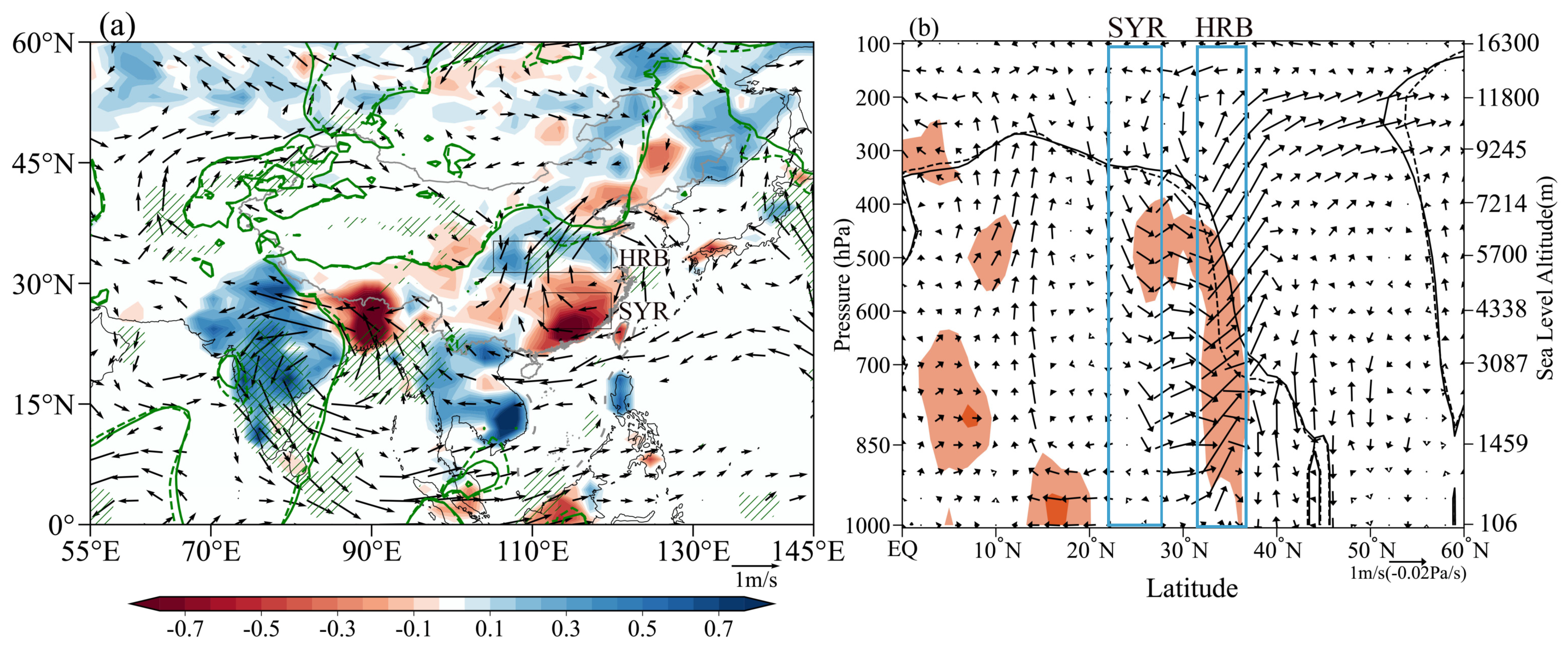
3.2. Mechanism Analysis

The two regions examined in this study exhibited disparities in terms of the dominant regional climate factors. Figure 2a shows the disparities in the circulation field between HSY and LSY. The position of the 0 m/s contours of southerly velocity clearly indicated that the impact range of the monsoon during HSY is considerably larger than during LSY, with its leading edge extending further northward. Analysis of the wind field disparities revealed significant southwest wind anomalies in HRB, which is situated at the boundary between the monsoon and westerly belts. This indicates that during HSY, the summer monsoon flow in this region becomes stronger, leading to increased precipitation in the HRB. However, the presence of an anticyclonic anomaly circulation in the central part of the EASM, known as the SYR, along with signs of weakened monsoon flow, hinders the occurrence of rainfall in the central part of the SYR. Consequently, this pattern favors the occurrence of floods in the southern region and droughts in the northern region.
The variation in the frontal position of the EASM is primarily caused by the southwest monsoon flow originating from the Bay of Bengal and the Western Pacific, as well as the position of the Western Pacific subtropical high. As shown in Figure 2a, the monsoon flow originates from the tropical Indian Ocean and the Western Pacific. Under the influence of the Western Pacific subtropical high, it turns northward toward China. During the HSY, there is a cyclonic anomaly circulation over the Bay of Bengal and India, which promotes an increased transport of water vapor toward the north. Meanwhile, an anticyclonic anomaly circulation exists over the Northwest Pacific and Southeastern China region, indicating that the Western Pacific subtropical high is positioned further north. This positioning facilitates the northward extension of the EASM.
In addition, the composite differences in the vertical wind fields along 113° E (Figure 2b) revealed that during the HSY, the 0 m/s contour of southerly velocity is generally located further north and at a higher altitude compared to the LSY. Notably, there is significant northward and upward motion above the HRB north of 30° N. This finding suggests that during the HSY, the range of the summer monsoon in summer is larger, leading to more extreme rainfall days in the HRB compared to the LSY. However, the abnormal subsidence flow over the SYR restricts convection and precipitation, resulting in a dry environment. This result supports the previous conclusion that extreme precipitation in the Chinese region during HSY often exhibits a “SDNF” pattern. Additionally, it suggests that the edge of the regional climate system may be more susceptible to external forcing, such as solar forcing, than its interior.
The above analysis suggests significant disparities in the response of monsoon edge and interior circulations to solar activity, which can account for the variations in precipitation patterns. To further investigate the underlying reasons for these circulation differences, we introduced the zonal circulation dipole index (ZCD) as the disparity in 700 hPa zonal winds between the HRB and SYR study areas. The correlation coefficient between ZCD and SSN was 0.30 for the period 1951–2018, passing the significance test at the 99% confidence level. We conducted wavelet power spectrum analysis to determine the dominant period. The Morlet wavelet was selected as the mother wavelet [58] and applied to both the ZCD and SSN. Figure 3d illustrates the global wavelet spectra of the ZCD and the corresponding annual SSN. It is evident that the ZCD exhibited a significant 11-year periodicity, similar to the SSN.
The scale-averaged wavelet power spectrum (SAWP) is a time series that represents the average energy spectrum within a specific frequency range. It is commonly used to detect whether one time series modulates another [58]. In this study, we utilized the SAWP to examine the relationship between the spectral energy variation of ZCD and SSN at the quasi-11-year scale. Figure 3e displays the time series of the quasi-11-year SAWP of ZCD and SSN for each year. The quasi-11-year spectral amplitude of the ZCD has become significant since the 1980s, indicating that the difference in circulation between the edge and interior of the EASM has exhibited a stronger quasi-11-year period after the 1980s compared to before. After 1979, there was an increase in satellite data, leading to significant improvements in observational data compared to the period before. Consequently, it became possible to detect the 11-year solar cycle with greater accuracy and precision. This finding is consistent with Figure 3b.
Results of the co-varying relationships between the SSN and summer ZCD, as depicted by the wavelet coherence and cross-wavelet, are presented in Figure 4. Wavelet coherence analysis (WTC) is a statistical tool used to measure the strength and significance of the relationship between two time series in different frequency bands. The cross-wavelet transform (XWT), constructed from two continuous wavelet transforms, can reveal their common power and relative phase shift [57,58]. If the dipole circulation index (ZCD) of the present study is related to the SC, their common power and a consistent or small phase lag should be detectable.
The WTC of the SSN and summer ZCD is shown in Figure 4a, showing a significant continuous common power in the 11-year band, and it became more significant after 1996. The 11-year common power between ZCD and SSN was more pronounced in XWT (Figure 4b). The relative phase relationship (arrows in Figure 4b) shows that in the sectors with significant common power (near the 11-year band), the SSN was primarily in phase with or slightly led the ZCD by about 1.4 years. This result suggests that for the majority of the 20th century, there was a strong synchronization or phase lock between the decadal oscillations of ZCD and SSN.
The zonally averaged circulation is a crucial component of atmospheric circulation and plays a significant role in its variations. To comprehend the intricate processes involved in the transmission of solar signals, a composite difference analysis of zonal wind variations from the stratosphere to the troposphere was conducted for the HSY and LSY. The analysis of the zonal wind difference between the HSY and LSY, as depicted in Figure 5a, revealed an abnormal wave pattern of “+ − + − +” in the composite difference of zonal wind across the middle-to-high latitudes along the meridional direction during summer throughout the troposphere. In the off-equatorial region, convection is intensified, while in the SYR, convection is weakened. Additionally, convection is strengthened in the HRB region. Conversely, the zonal wind composite difference in the middle-to-high latitudes along 113° E for the stratosphere, from 30 hPa to 5 hPa, exhibited a wave pattern of “− + −”. This pattern is essentially opposite to that observed in the troposphere. It demonstrates that the positive zonal wind response in the upper levels of the subtropical region is accompanied by a negative wind response in the lower levels.
However, the scale of waves in the stratosphere is usually larger than that in the troposphere, indicating that the signals in the stratosphere propagate at a slower pace compared to those in the troposphere (e.g., [60]). This could cause misalignment of the anomaly centers of the stratosphere and the troposphere. Therefore, the above finding is consistent with previous studies [60].
To examine the contrasting phase change between anomalies in the stratosphere and troposphere, the composite difference of zonal wind speeds at 10 hPa (113° E, 33° N) and 700 hPa (113° E, 18° N) can be utilized. Figure 5b illustrates the time series of zonal wind differences at 10 hPa and 700 hPa. The correlation coefficient between the zonal wind difference and the sunspot number (SSN) was 0.25, which is significant at the 96% confidence level. Additionally, the correlation coefficient between the zonal wind difference and the first principal component (PC1) of R20mm was 0.34, with a p-value of 0.004. The correlation coefficient between zonal wind speeds at 10 hPa and SSN was 0.19, while at 700 hPa it was −0.17. Therefore, the composite difference of zonal wind speeds at 10 hPa (113° E, 33° N) and 700 hPa (113° E, 18° N) was more strongly correlated with SSN compared to a single region.
The spatial distribution of correlation coefficients between the zonal wind difference series and R20mm (Figure 5c) illustrated that significant differences in the zonal wind between the troposphere and stratosphere in the subtropical region result in HRB experiencing a higher number of extreme precipitation days, while SYR has fewer extreme precipitation days. This finding potentially provides further support for the association between the vertical difference of zonal wind over the subtropics and the “SDNF” extreme precipitation pattern in China. There may be an inherent connection between the variations in zonal wind from the stratosphere to the troposphere and the 11-year SC. The East Asian subtropical westerly jet, located in the convergence zone of warm and cold air masses at mid-latitudes in the Northern Hemisphere (NH), along with the upper-level front, plays a crucial role in determining the pathways of storm systems. These storm systems travel along specific pathways, leading to the occurrence, development, or interaction of cyclones or anticyclones with circulation systems at different latitudes. As a result, this dynamic process between the stratosphere and troposphere significantly influences the occurrence of extreme heavy precipitation weather events in East Asia.

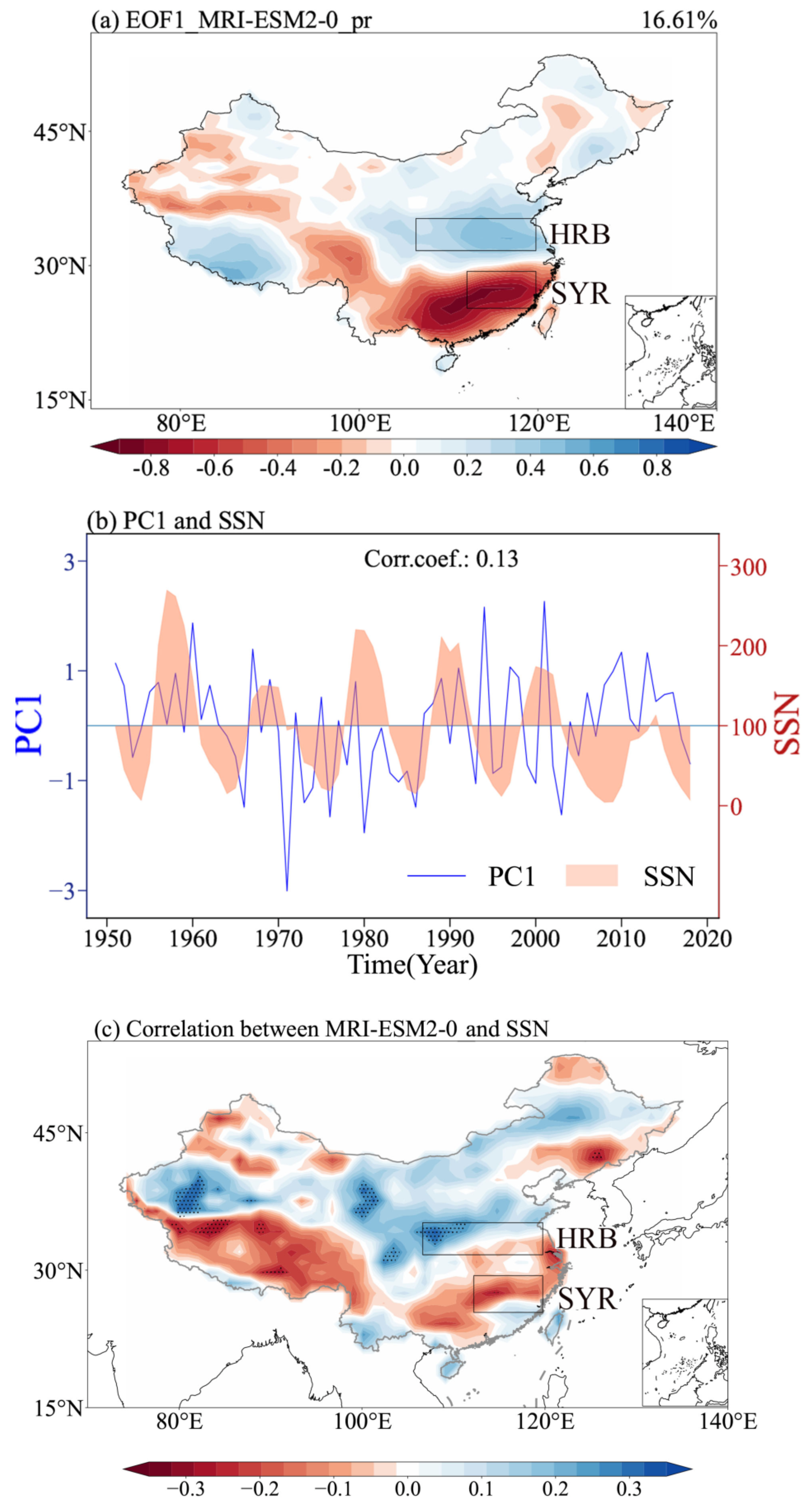
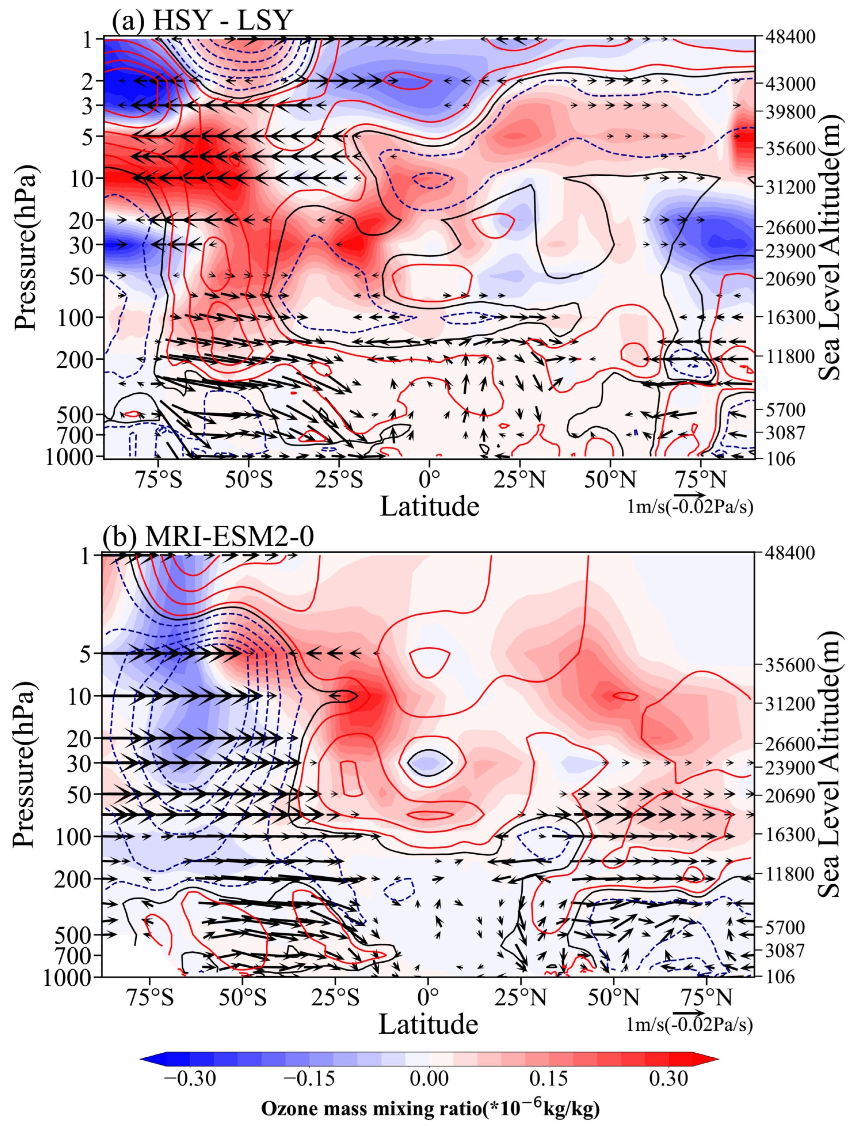
3.3. Solar Signals in CMIP6 Simulations

In order to verify the authenticity and significance of the responses of precipitation and atmospheric circulation to the 11-year solar signal in observations, we assessed the simulation capabilities of five models (Table 1) through a DAMIP hist-sol experiment, where hist-sol simulations are driven by solar forcing only. These experiments focused on the climate response to SC since the Industrial Revolution. In this study, we investigated variations of precipitation, atmospheric circulation, and ozone in these experiments from 1951 to 2018. Among the five models, the EOF1 mode of MRI-ESM2-0 (Figure 6a) closely resembled the observed EOF1 of R20mm (Figure 1a), with a spatial correlation coefficient of 0.70. Additionally, the PC1 of MRI-ESM2-0 exhibited the highest correlation with SSN among the five models. The MRI-ESM2-0 model effectively simulated the primary modes of EOF and their temporal evolution characteristics of summer precipitation in China from 1951 to 2018.
Figure 6a shows a “SDNF” pattern in the dominant mode of the precipitation field for the hist-sol of the MRI-ESM2-0 model during the summer from 1951 to 2018. The correlation coefficient between the PC1 series and SSN was 0.13 (Figure 6b). Additionally, the correlation distribution between SSN and the MRI-ESM2-0 precipitation also exhibited the “SDNF” pattern (Figure 6c). The EOF1 of the MRI-ESM2-0 model, along with its correlation distribution with SSN, demonstrated a distinct “SDNF” pattern that closely resembled that of R20mm (Figure 1a,c). This indicates that the sol experiment data from the MRI-ESM2-0 model can effectively simulate this long-term variation trend.
For atmospheric circulation associated with the EOF1, we compared the similarities and differences between the observations in Figure 2a and the hist-sol results of the MRI-ESM2-0 model. Figure 7 illustrates that, over the past 70 years, the MRI-ESM2-0 model has successfully reproduced the observed precipitation patterns at a climatological scale. Specifically, during the HSY period, there was a significant amount of precipitation in the HRB region, while less precipitation was observed in the SYR. The 700 hPa wind field showed a significant southwest wind anomaly in the HRB region, while a cyclonic anomaly circulation pattern was observed in the SYR. Overall, the model reasonably reproduced the spatial distribution characteristics of precipitation, circulation, and horizontal wind fields across a large area of China.

4. Discussion and Conclusions

Previous studies showed that the anomalies in atmospheric circulation in the stratosphere and troposphere may be linked to the response of stratospheric ozone to SC (e.g., [25,30,33,61]). Figure 8 illustrates the vertical cross-section of composite differences in ozone, temperature, and wind fields in summer for the HSY and LSY in observations and models. In observation (Figure 8a) during the HSY, there was an increased concentration of ozone and higher temperatures in the SH (winter hemisphere), which aligns with the findings of Hood et al. [33]. This phenomenon includes a negative meridional gradient of temperature, intensifying westerlies, and a vertical temperature anomaly with warm upper and cold lower layers, i.e., a temperature inversion layer, suppressing convection and facilitating a sinking movement. The northward downward airflow associated with this process enhances convective activity in the equatorial region. Additionally, this airflow transports warm anomalies to the upper troposphere in the NH, leading to anomalous warmth near the tropical and subtropical tropopause. Consequently, convection over the subtropical region is inhibited.
Notably, there is a distinct anomaly of downward motion observed around 20–30° N, which is unfavorable for precipitation and favorable for a high-pressure anomaly, specifically enhancing the Western Pacific subtropical high. This enhanced high-pressure system in the Western Pacific will promote precipitation on its northwest side. Additionally, it is evident that there is a decrease in ozone levels in the middle stratosphere of the NH during the HSY, which is in contrast to the trend observed in the Southern Hemisphere. The warming anomaly in the lower stratosphere at mid-latitudes in the NH is weaker compared to that in the Southern Hemisphere. Additionally, there is a strong cold anomaly in the tropopause over the 60–80° N region, which results in westerly anomalies over the mid-latitudes. These westerly anomalies coincide with the existing westerly winds in the northern part of the subtropical high, leading to the formation of a robust cyclonic anomaly and upward motion around the 30–45° N region. Consequently, an anomalous circulation pattern was established, characterized by sinking air south of 30° N and ascending air north of it.
Therefore, it can be speculated that a fundamental driver of precipitation and circulation patterns is the significant response of stratospheric ozone to solar forcing. The impact of ozone and temperature responses has also been confirmed in several studies (e.g., [62]).
For the hist-sol results of the MRI-ESM2-0 model, we evaluated the performance of the MRI-ESM2-0 model in simulating various meteorological variables’ responses in Figure 8b. The hist-sol simulation results can roughly reproduce the observed solar signals in the stratosphere and the troposphere, including the ozone response in the stratosphere and the wave train in the troposphere. In comparison to Figure 8a, the simulated horizontal meridional wind difference in the stratosphere (5–30 hPa) of the SH exhibited an anti-phase relationship with the observed. This anti-phase behavior was also evident in the NH stratosphere (50–200hPa). Additionally, when examining the simulated SH polar region, it became apparent that the stratospheric ozone significantly decreased in comparison to the observed, accompanied by an expansion of the cold anomaly range reaching approximately 30° S. Furthermore, the simulated warm anomalies in the NH were notably higher compared to those depicted in Figure 8a. The temperature increase in the NH is associated with an elevated ozone concentration in the local upper atmosphere and its transport in the SH.
This work investigated the relationship between the 11-year SC and the occurrence of the “SDNF” pattern in China during the past 6 SCs based on 68 years of extreme precipitation data and the corresponding SSN data. The first EOF principal mode of R20mm (monthly count of days with precipitation ≥ 20 mm) in China during summer from 1951 to 2018, exhibiting a distinct distribution of “SDNF”, was revealed to be modulated by the 11-year SC. The study also explored the dynamic mechanism underlying this relationship. Positive or negative correlations were also observed in areas both north and south of the Yangtze River. Based on the evaluation of precipitation modeling capabilities in China from 1951 to 2018, using the hist-sol of the MRI-ESM2-0 model in the DAMIP project within CMIP6, the solar modulation effect on the “SDNF” pattern in precipitation was confirmed.
The strengthening and northward expansion of the EASM during the HSY period resulted in an increased number of days with extreme precipitation in the HRB compared to the LSY period. This phenomenon likely contributed to inter-decadal oscillations in precipitation at the HRB. Additionally, anomalous descending over the SYR suppressed convection and precipitation, creating a dry environment.
Analysis of the zonal wind anomalies during HSY and LSY revealed a complementary relationship between the positive response in the upper troposphere and the negative response in the lower troposphere in the subtropical region. The zonal wind difference between the upper and lower troposphere in the subtropics exhibited a positive correlation with the pattern of drought in the southern regions and floods in the northern regions. Further investigation suggested that the negative gradient of ozone and temperature in the stratosphere (20–40° N) precisely corresponds to the positive anomalies in the zonal wind, resulting in abnormal easterly winds in the tropical stratosphere of the NH. These abnormal winds subsequently propagate downwards, leading to a warm anomaly at the 100 hPa level in the tropical region. This suppresses convection below and induces the propagation of anomalous meridional wind in a “+ − +” wave pattern. Kodera [63] indicated that the solar influence on monsoon activity originates from the stratosphere, not the troposphere, through the modulation of tropical upwelling. Our results suggested that the solar modulation effect is due to the response of stratospheric ozone to variations in solar radiation. The ozone response should be related to solar-induced variations in the Brewer–Dobson circulation (BDC) [64].
Further analysis revealed that the potential pathway of the “top-down” mechanism is as follows: SSN → ozone → temperature → circulation (in the EASM region) → extreme precipitation. Ozone plays a crucial role as an intermediary, connecting solar activity with the tropospheric climate. The solar signal is transmitted vertically from the upper atmosphere to the stratosphere, affecting ozone concentration and, subsequently, influencing temperature distribution. Lower temperatures at higher levels enhance convective processes, which have implications for the occurrence of extreme precipitation events.

Author Contributions

J.L., investigation, software, data curation, methodology, writing—original draft; L.Z., visualization, supervision; J.W. and L.Z., funding acquisition, conceptualization, resources, project administration; Z.X., validation, formal analysis. All authors have read and agreed to the published version of the manuscript.

Funding

This research is supported by the National Natural Science Foundation of China (Grant Nos. 42075040 and 42274217) and the Strategic Priority Research Program of the Chinese Academy of Sciences (XDA23090102).

Institutional Review Board Statement

Not applicable.

Informed Consent Statement

Not applicable.

Data Availability Statement

The observed gridded precipitation data were taken from the Expert Team on Climate Change Detection and Indices (ETCCDI) dataset, available at: https://www.metoffice.gov.uk/hadobs/hadex3/download.html accessed on 1 January 2020. Zonal and meridional winds, vertical velocities, air temperature, and ozone can be downloaded from the fifth generation of the ECMWF (ERA5) reanalysis dataset at: https://cds.climate.copernicus.eu/cdsapp#!/dataset/reanalysis-era5-pressure-levels-monthly-means?tab=overview accessed on 1 January 2020. This study used gridded monthly data for precipitation, zonal and meridional winds, vertical velocities, air temperature, and ozone from Phase 6 of the Coupled Model Intercomparison Project (CMIP6). CMIP6 simulations are available through the CMIP6 Search Interface (https://esgf-node.llnl.gov/search/cmip6/) accessed on 1 January 2020.

Acknowledgments

We thank the joint World Meteorological Organization (WMO) Central Calibration Laboratory (CCL)/World Climate Research Program (WCRP)/The Joint WMO/IOC Technical Commission for Oceanography and Marine Meteorology (JCOMM) Expert Team on Climate Change Detection and Indices (ETCCDI) for the extreme precipitation datasets. We acknowledge Sunspot Index and Long-term Solar Observations (SILSO) for the SSN data and ECMWF for the ozone, wind, and temperature data. We thank the Detection and Attribution Model Intercomparison Project (DAMIP) and the WCRP’s Working Group on Coupled Modeling and the climate modeling groups for producing and making available CMIP6 model output.

Conflicts of Interest

The authors declare no conflict of interest.

References

  1. Lean, J.L. Estimating solar irradiance since 850 CE. Earth Space Sci. 2018, 5, 133–149. [Google Scholar] [CrossRef]
  2. Wang, J.; Zhao, L.; Xiao, Z.; Zhang, P.; Ren, Z.; Zong, W.; Qi, J.; Huang, C.; Xu, Y.; Lu, Y. Energy transmission processes in the effectuation chain of solar forcing to the terrestrial atmosphere—A review. Front. Earth Sci. 2023, 11, 1164636. [Google Scholar] [CrossRef]
  3. Gray, L.J.; Beer, J.; Geller, M.; Haigh, J.D.; Lockwood, M.; Matthes, K.; Cubasch, U.; Fleitmann, D.; Harrison, G.; Hood, L.; et al. Solar influences on climate. Rev. Geophys. 2010, 48, RG4001. [Google Scholar] [CrossRef]
  4. Seppälä, A.; Matthes, K.; Randall, C.; Mironova, I. What is the solar influence on climate?—Overview of activities during CAWSES-II. Prog. Earth Planet. Sci. 2014, 1, 24. [Google Scholar] [CrossRef]
  5. Gillett, N.P.; Shiogama, H.; Funke, B.; Hegerl, G.; Knutti, R.; Matthes, K.; Santer, B.D.; Stone, D.; Tebaldi, C. The Detection and Attribution Model Intercomparison Project (DAMIP v1.0) contribution to CMIP6. Geosci. Model Dev. 2016, 9, 3685–3697. [Google Scholar] [CrossRef]
  6. Ineson, S.; Scaife, A.; Knight, J.; Manners, J.C.; Dunstone, N.J.; Gray, L.J.; Haigh, J.D. Solar forcing of winter climate variability in the Northern Hemisphere. Nat. Geosci. 2011, 4, 753–757. [Google Scholar] [CrossRef]
  7. Matthes, K. Solar cycle and climate predictions. Nat. Geosci. 2011, 4, 735–736. [Google Scholar] [CrossRef]
  8. Kodera, K.; Kuroda, Y. Dynamical response to the solar cycle. J. Geophys. Res. 2002, 107, 4749. [Google Scholar] [CrossRef]
  9. Lockwood, M. Solar change and climate: An update in the light of current exceptional solar minimum. Proc. R. Soc. A 2010, 466, 303–329. [Google Scholar] [CrossRef]
  10. Zolotova, N.V.; Ponyavin, D.I. Is the new Grand mini-mum in progress? J. Geophys. Res. Space Phys. 2014, 119, 3281–3285. [Google Scholar] [CrossRef]
  11. Chiodo, G.; Garcíaherrera, R.; Calvo, N.; Vaquero, J.M.; A Añel, J.; Barriopedro, D.; Matthes, K. The impact of a future solar minimum on climate change projections in the Northern Hemisphere. Environ. Res. Lett. 2016, 11, 034015. [Google Scholar] [CrossRef]
  12. Kodera, K.; Thiéblemont, R.; Yukimoto, S.; Matthes, K. How can we understand the global distribution of the solar cycle signal on the Earth’s surface? Atmos. Chem. Phys. 2016, 16, 12925–12944. [Google Scholar] [CrossRef]
  13. Ogurtsov, M. Long-Term Variability of Summer Temperature in the Southern Part of South America—Is There a Connection with Changes in Solar Activity? Atmosphere 2022, 13, 1360. [Google Scholar] [CrossRef]
  14. Marsh, N.D.; Svensmark, H. Cosmic Rays, Clouds, and Climate. Space Sci. Rev. 2000, 94, 215–230. [Google Scholar] [CrossRef]
  15. Usoskin, I.G.; Schuessler, M.; Solanki, S.K.; Mursula, K. Solar activity, cosmic rays, and Earth’s temperature: A millennium-scale comparison. J. Geophys. Res. 2005, 110, A10102. [Google Scholar] [CrossRef]
  16. Veretenenko, S.; Ogurtsov, M.G. Stratospheric circumpolar vortex as a link between solar activity and circulation of the lower atmosphere. Geomagn. Aeron. 2012, 52, 937–943. [Google Scholar] [CrossRef]
  17. Sfîcă, L.; Beck, C.; Nita, A.I.; Voiculescu, M.; Birsan, M.V.; Philipp, A. Cloud cover changes driven by atmospheric circulation in Europe during the last decades. Int. J. Climatol. 2021, 41 (Suppl. S1), 2211–2230. [Google Scholar] [CrossRef]
  18. CMA Climate Change Centre. Blue Book on Climate Change in China; Science Press: Beijing, China, 2022. [Google Scholar]
  19. Huang, R.H.; Xu, Y.H.; Zhou, L.T. The interdecadal variation of summer precipitations in China and the drought trend in North China. Plateau Meteor. 1999, 18, 465–476. (In Chinese) [Google Scholar]
  20. Herman, J.R.; Goldberg, R.A. Sun, Weather and Climate; University Press of the Pacific: Forest Grove, OR, USA, 2005; 376p. [Google Scholar]
  21. Zhao, L.; Wang, J.; Zhao, H. Solar cycle signature in decadal variability of monsoon precipitation in China. J. Meteorol. Soc. Jpn. 2012, 90, 1–9. [Google Scholar] [CrossRef]
  22. Jin, C.; Liu, J.; Wang, B.; Yan, M.; Ning, L. Decadal Variations of the East Asian Summer Monsoon Forced by the 11-Year Insolation Cycle. J. Clim. 2019, 32, 2735–2745. [Google Scholar] [CrossRef]
  23. Ma, H.; Chen, H.; Gray, L.; Zhou, L.; Li, X.; Wang, R.; Zhu, S. Changing response of the North Atlantic/European winter climate to the 11 year solar cycle. Environ. Res. Lett. 2019, 13, 034007. [Google Scholar] [CrossRef]
  24. Wang, J.; Zhao, L. Statistical tests for a correlation between decadal variation in June precipitation in China and sunspot number. J. Geophys. Res. Atmos. 2012, 117, D23117. [Google Scholar] [CrossRef]
  25. Zhao, L.; Wang, J.; Liu, H.; Xiao, Z. Amplification of solar signal in summer monsoon rainband in China by a synergistic action of different dynamical responses. J. Meteor. Res. 2017, 31, 61–72. [Google Scholar] [CrossRef]
  26. Barde, V.; Upadhyay, A.; Bulusu, J.; Dimri, A.P. Impact of solar variability on Indian summer monsoon through large scale circulations. J. Atmos. Sol. Terr. Phys. 2023, 252, 1364–6826. [Google Scholar] [CrossRef]
  27. Lu, Z.; Zhang, Q.; Miller, P.A.; Zhang, Q.; Berntell, E.; Smith, B. Impacts of large-scale Sahara solar farms on global climate and vegetation cover. Geophys. Res. Lett. 2021, 48, e2020GL090789. [Google Scholar] [CrossRef]
  28. Maghrabi, A.H.; Alamoudi, H.A.; Alruhaili, A.S. Investigation of a Possible Link between Solar Activity and Climate Change in Saudi Arabia: Rainfall Patterns. Atmos. Clim. Sci. 2023, 13, 478–490. [Google Scholar] [CrossRef]
  29. Haigh, J.D. The impact of solar variability on climate. Science 1996, 272, 981–984. [Google Scholar] [CrossRef] [PubMed]
  30. Haigh, J.D. The role of stratospheric ozone in modulating the solar radiative forcing of climate. Nature 1994, 370, 544–546. [Google Scholar] [CrossRef]
  31. Haigh, J.D.; Blackburn, M.; Day, R. The response of tropospheric circulation to perturbations in lower-stratospheric temperature. J. Clim. 2005, 18, 3672–3685. [Google Scholar] [CrossRef]
  32. Shindell, D.; Rind, D.; Balachandran, N.; Lean, J.; Lonergan, P. Solar cycle variability, ozone, and climate. Science 1999, 284, 305–308. [Google Scholar] [CrossRef] [PubMed]
  33. Hood, L.L.; Misios, S.; Mitchell, D.M.; Rozanov, E.; Gray, L.J.; Tourpali, K.; Matthes, K.; Schmidt, H.; Chiodo, G.; Thieblemont, R.; et al. Solar signals in CMIP-5 simulations: The ozone response. Q. J. R. Meteorol. Soc. 2015, 141, 2670–2689. [Google Scholar] [CrossRef]
  34. Roy, I.; Haigh, J.D. Solar cycle signals in sea level pressure and sea surface temperature. Atmos. Chem. Phys. 2010, 10, 3147–3153. [Google Scholar] [CrossRef]
  35. Misios, S.; Mitchell, D.M.; Gray, L.J.; Tourpali, K.; Matthes, K.; Hood, L.; Schmidt, H.; Chiodo, G.; Thiéblemont, R.; Rozanov, E.; et al. Solar signals in CMIP-5 simulations: Effects of atmosphere-ocean coupling. Q. J. R. Meteorol. Soc. 2016, 142, 928–941. [Google Scholar] [CrossRef]
  36. Meehl, G.A.; Arblaster, J.M.; Matthes, K.; Sassi, F.; van Loon, H. Amplifying the Pacific Climate System Response to a Small 11-Year Solar Cycle Forcing. Science 2009, 325, 1114–1118. [Google Scholar] [CrossRef] [PubMed]
  37. Newell, R.E.; Zhu, Y.; Browell, E.V.; Read, W.G.; Waters, J.W. Walker circulation and tropical upper tropospheric water vapor. J. Geophys. Res. Atmos. 1996, 101, 1961–1974. [Google Scholar] [CrossRef]
  38. Tanaka, H.L.; Ishizaki, N.; Kitoh, A. Trend and interannual variability of Walker, monsoon and Hadley circulations defined by velocity potential in the upper troposphere. Tellus A 2004, 56, 250–269. [Google Scholar] [CrossRef]
  39. Tanaka, H.L.; Ishizaki, N.; Nohara, D. Intercomparison of the intensities and trends of Hadley, Walker and monsoon circulations in the global warming projections. SOLA 2005, 1, 77–80. [Google Scholar] [CrossRef]
  40. Misios, S.; Gray, L.J.; Knudsen, M.F.; Karoff, C.; Schmidt, H.; Haigh, J.D. Slowdown of the Walker circulation at solar cycle maximum. Proc. Natl. Acad. Sci. USA 2019, 116, 7186–7191. [Google Scholar] [CrossRef] [PubMed]
  41. Misios, S.; Kasoar, M.; Kasoar, E.; Gray, L.; Haigh, J.; Stathopoulos, S.; Kourtidis, K.; Myhre, G.; Olivié, D.; Shindell, D.; et al. Similar patterns of tropical precipitation and circulation changes under solar and greenhouse gas forcing. Environ. Res. Lett. 2021, 16, 104045. [Google Scholar] [CrossRef]
  42. Huo, W.; Xiao, Z.; Zhao, L. Phase-Locked Impact of the 11-year solar cycle on tropical pacific decadal variability. J. Clim. 2022, 36, 421–439. [Google Scholar] [CrossRef]
  43. Dunn, R.J.H.; Donat, M.G.; Alexander, L.V. Investigating uncertainties in global gridded datasets of climate extremes. Clim. Past 2014, 10, 2171–2199. [Google Scholar] [CrossRef]
  44. Dunn, R.J.H.; Alexander, L.V.; Donat, M.G.; Zhang, X.; Bador, M.; Herold, N.; Lippmann, T.; Allan, R.; Aguilar, E.; Barry, A.A.; et al. Development of an updated global land in-situ-based dataset of temperature and precipitation extremes: HadEX3 JGR-A. J. Geophys. Res. Atmos. 2020, 125, e2019JD032263. [Google Scholar] [CrossRef]
  45. Eyring, V.; Bony, S.; Meehl, G.A.; Senior, C.A.; Stevens, B.; Stouffer, R.J.; Taylor, K.E. Overview of the Coupled Model Intercomparison Project Phase 6 (CMIP6) experimental design and organization. Geosci. Model Dev. 2016, 9, 1937–1958. [Google Scholar] [CrossRef]
  46. Mitchell, D.M.; Misios, S.; Gray, L.J.; Tourpali, K.; Matthes, K.; Hood, L.; Schmidt, H.; Chiodo, G.; Thiéblemont, R.; Rozanov, E.; et al. Solar signals in CMIP-5 simulations: The stratospheric pathway. Q. J. R. Meteorol. Soc. 2015, 141, 2390–2403. [Google Scholar] [CrossRef]
  47. Yukimoto, S.; Koshiro, T.; Kawai, H.; Oshima, N.; Yoshida, K.; Urakawa, S.; Tsujino, H.; Deushi, M.; Tanaka, T.; Hosaka, M.; et al. MRI MRI-ESM2.0 Model Output Prepared for CMIP6 DAMIP Hist-Sol; Earth System Grid Federation: Online, 2019. [Google Scholar] [CrossRef]
  48. Kelley, M.; Schmidt, G.A.; Nazarenko, L.; Bauer, S.E.; Ruedy, R.; Russell, G.L.; Ackerman, A.S.; Aleinov, I.; Bauer, M.; Bleck, R.; et al. GISS-E2.1: Configurations and climatology. J. Adv. Model. Earth Syst. 2020, 12, e2019MS002025. [Google Scholar] [CrossRef]
  49. Swart, N.C.; Cole, J.N.S.; Kharin, V.V.; Lazare, M.; Scinocca, J.F.; Gillett, N.P.; Anstey, J.; Arora, V.; Christian, J.R.; Jiao, Y.; et al. CCCma CanESM5 Model Output Prepared for CMIP6 DAMIP Hist-Sol; Earth System Grid Federation: Online, 2019. [Google Scholar] [CrossRef]
  50. Shiogama, H. MIROC MIROC6 Model Output Prepared for CMIP6 DAMIP Hist-CO2; Earth System Grid Federation: Online, 2019. [Google Scholar] [CrossRef]
  51. NASA Goddard Institute for Space Studies (NASA/GISS). NASA-GISS GISS-E2.1G Model Output Prepared for CMIP6 DAMIP Hist-Sol; Earth System Grid Federation: Online, 2018. [Google Scholar] [CrossRef]
  52. NASA Goddard Institute for Space Studies (NASA/GISS). NASA-GISS GISS-E2-2-G Model Output Prepared for CMIP6 DAMIP Hist-Sol; Earth System Grid Federation: Online, 2021. [Google Scholar] [CrossRef]
  53. Jolliffe, I.T. Principal components in regression analysis. In Principal Component Analysis; Springer: Cham, Switzerland, 1986. [Google Scholar]
  54. Bjornsson, H.; Venegas, S. A manual for EOF and SVD analyses of climatic data. CCGCR Rep. 1997, 97, 112–134. [Google Scholar]
  55. Ionita, M.; Lohmann, G.; Rimbu, N.; Scholz, P. Dominant modes of Diurnal Temperature Range variability over Europe and their relationships with large-scale atmospheric circulation and sea surface temperature anomaly patterns. J. Geophys. Res. Atmos. 2012, 117, D15111. [Google Scholar] [CrossRef]
  56. Zhang, Z.; Moore, J.C. (Eds.) Chapter 6—Empirical Orthogonal Functions. In Mathematical and Physical Fundamentals of Climate Change; Elsevier: Amsterdam, The Netherlands, 2015; pp. 161–197. [Google Scholar]
  57. Grinsted, A.; Moore, J.C.; Jevrejeva, S. Application of the cross wavelet transform and wavelet coherence to geophysical time series. Nonlinear Process. Geophys. 2004, 11, 561–566. [Google Scholar] [CrossRef]
  58. Torrence, C.; Compo, G.P. A practical guide to wavelet analysis. Bull. Am. Meteorol. Soc. 1998, 79, 61–78. [Google Scholar] [CrossRef]
  59. Metropolis, N.; Rosenbluth, A.W.; Rosenbluth, M.N.; Teller, A.H.; Teller, E. Equation of State Calculations by Fast Computing Machines. J. Chem. Phys. 1953, 21, 1087–1092. [Google Scholar] [CrossRef]
  60. Baldwin, M.P.; Gray, L.J.; Dunkerton, T.J.; Hamilton, K.; Haynes, P.H.; Randel, W.J.; Holton, J.R.; Alexander, M.J.; Hirota, I.; Horinouchi, T.; et al. The quasi-biennial oscillation. Rev. Geophys. 2001, 39, 179–229. [Google Scholar] [CrossRef]
  61. Baldwin, M.P.; Stephenson, D.B.; Thompson, D.W.; Dunkerton, T.J.; Charlton, A.J.; O’Neill, A. Stratospheric memory and skill of extended-range weather forecasts. Science 2003, 301, 636–640. [Google Scholar] [CrossRef] [PubMed]
  62. Bednarz, E.M.; Maycock, A.C.; Braesicke, P.; Telford, P.J.; Abraham, N.L.; Pyle, J.A. Separating the role of direct radiative heating and photolysis in modulating the atmospheric response to the amplitude of the 11-year solar cycle forcing. Atmos. Chem. Phys. 2019, 19, 9833–9846. [Google Scholar] [CrossRef]
  63. Kodera, K. Solar influence on the Indian Ocean Monsoon through dynamical processes. Geophys. Res. Lett. 2004, 31, L24209. [Google Scholar] [CrossRef]
  64. Hood, L.L.; Soukharev, B.E. The lower-stratospheric response to 11-Yr solar forcing: Coupling to the tropospheretd-Ocean response. J. Atmos. Sci. 2012, 69, 1841–1864. [Google Scholar] [CrossRef]
Figure 1. (a) Spatial distribution of the EOF1 mode of R20mm for summer from 1951 to 2018. (b) Standardized time series of unfiltered (solid blue line)/9–13-year band-pass-filtered (thick blue line) PC1 and corresponding annual SSN (shaded in red). (c) Spatial distribution of linear correlations between the summer mean R20mm at each grid and the corresponding annual SSN for the period 1951–2018. Black dots indicate regions that pass the 95% significance test. The middle and bottom rectangles outline HRB and SYR, respectively. (d) Spatial distribution of 68-year (1951–2018) mean R20mm (shade; units: d) and 700 hPa horizontal wind (vector arrows; units: 10 m/s) for summer averaged over the period 1951–2018. Thick black contours are the mean southerly velocity contours of 0 m/s, representing the margin of the EASM.
Atmosphere 15 00175 g001
Figure 2. Composite difference map (vector arrows) of summer wind between the HSY and LSY for the period 1951–2018, showing: (a) horizontal wind (units: m/s) at a 700 hPa constant pressure surface, composite differences between HSY and LSY extreme precipitation R20mm (color-filled plots, units: days), and (b) meridional wind (units: m/s) and vertical pressure wind (units: −0.02 Pa/s, so that positive is upward) along the longitude 113° E cross-section. The thick solid/long dashed contours indicate the HSY/LSY mean southerly velocity contours of 0 m/s, representing the margin of the EASM. Dark and light green and red shaded areas indicate areas where meridional wind differences are significant at 95% and 80% confidence levels (t-test).
Atmosphere 15 00175 g002
Figure 3. The 1951–2018 summer-averaged (a) dipole circulation index (ZCD; blue solid line) and SSN (red shaded) time series. (b) ZCD wavelet power spectrum (Morlet wavelet): the blue solid line denotes the region where the confidence level exceeds 95%. (c) Same as (b) but changed to SSN. (d) Global wavelet (Morlet wavelet) spectra of ZCD (blue solid line) and SSN (red solid line) for the current year (test lines, dashed lines, representing the 95% confidence level). (e) Quasi-11-year (9–13 years) scale-averaged wavelet power spectrum (SAWP) (ZDC: blue solid line, SSN: red solid line) with test lines, dashed lines, representing the 95% confidence level.
Atmosphere 15 00175 g003
Figure 4. (a) Wavelet coherency and (b) cross-wavelet transforms’ analysis showing the relations between the summer-averaged dipole circulation index (ZCD) from 1951 to 2018 and the corresponding annual SSN. The relative phase relationship is shown by arrows (with in-phase pointing right, anti-phase pointing left, and SSN leading precipitation by 90° pointing straight down). The 95% significance level against red noise is shown as a thick contour.
Atmosphere 15 00175 g004
Figure 5. (a) Latitude–pressure cross-section of the composite difference in zonal wind between the HSY and LSY along 113° E from 1951 to 2018 (unit: m s−1). The light and dark shading indicate regions where the zonal wind t-test exceeds the 80% and 95% confidence levels, respectively, represented by positive (red) and negative (blue) colors. (b) SSN time series (red solid line) averaged over summer from 1951 to 2018: PC1 of extreme precipitation R20mm in China (blue solid line) and the zonal wind difference time series between 10 hPa and 700 hPa (blue shading). (c) Spatial distribution of correlation coefficients between R20mm and the zonal wind difference series averaged over summer from 1951 to 2018, with the dotted region being the area where the t-test for zonal wind differences at 10 hPa and 700 hPa exceeds the 95% confidence level.
Atmosphere 15 00175 g005
Figure 6. (a) Spatial distribution of the EOF1 mode of precipitation in MRI-ESM2-0 models for summer from 1951 to 2018. (b) The time series of PC1 (solid blue line) and SSN (shaded in red) from 1951 to 2018. (c) Spatial correlation of precipitation fields for SSN and MRI-ESM2-0 models.
Atmosphere 15 00175 g006
Figure 7. Similar to Figure 2a but using data from the MRI-ESM2-0 model.
Atmosphere 15 00175 g007
Figure 8. (a) Mean difference of the summer ozone mixing ratio (color-filled plots, units: 10−6 kg/kg), temperature (contours, units: °C), and vertical meridional circulation (vector arrows) averaged along 105–120° E of unfiltered summer horizontal meridional wind (units: 1 m/s) and vertical pressure velocity (units: −0.02 Pa/s, so that positive is upward) between the HSY and the LSY from 1951 to 2018. (b) Similar to (a) but using data from the MRI-ESM2-0 model.
Atmosphere 15 00175 g008
Table 1. CMIP6 models.
ModelHorizontal (°)LevelsModel Top (hPa)Reference
CanESM52.8 × 2.8491Swart et al., 2019 [49]
MIROC61.4 × 1.4810.004Shiogama et al., 2019 [50]
GISS-E2-1-G2.5 × 2.0400.1(NASA/GISS), 2018 [51]
GISS-E2-2-G2.0 × 2.51020.002(NASA/GISS), 2021 [52]
MRI-ESM2-01.1 × 1.1800.01Yukimoto et al., 2019 [47]
Table 2. HSY or LSY over the period 1951–2018.
SC NumberCycle YearsHSYLSY
181944–1954 1953, 1954
191954–19641956, 1957, 19581955, 1963, 1964
201964–19761967, 1968, 19691965, 1975, 1976
211976–19861978, 1979, 19801977, 1985, 1986
221986–19961988, 1989, 19901987, 1995, 1996
231996–20081999, 2000, 20011997, 2007, 2008
242008–20192013, 2014, 20152009, 2018
Total years (1951–2018)681819
Disclaimer/Publisher’s Note: The statements, opinions and data contained in all publications are solely those of the individual author(s) and contributor(s) and not of MDPI and/or the editor(s). MDPI and/or the editor(s) disclaim responsibility for any injury to people or property resulting from any ideas, methods, instructions or products referred to in the content.

