Article

Influences of Cloud Microphysics on the Components of Solar Irradiance in the WRF-Solar Model

1
Environmental & Climate Sciences Department, Brookhaven National Laboratory, Upton, NY 11973, USA
2
Atmospheric Science Department, Cornell University, Ithaca, NY 14853, USA
3
Atmospheric Science and Global Change Division, Pacific Northwest National Laboratory, Richland, WA 99352, USA
4
National Renewable Energy Laboratory, Golden, CO 80401, USA
*
Authors to whom correspondence should be addressed.
Atmosphere 2024, 15(1), 39; https://doi.org/10.3390/atmos15010039
Submission received: 1 December 2023 / Revised: 22 December 2023 / Accepted: 24 December 2023 / Published: 28 December 2023

Abstract

:
An accurate forecast of Global Horizontal solar Irradiance (GHI) and Direct Normal Irradiance (DNI) in cloudy conditions remains a major challenge in the solar energy industry. This study focuses on the impact of cloud microphysics on GHI and its partition into DNI and Diffuse Horizontal Irradiance (DHI) using the Weather Research and Forecasting model specifically designed for solar radiation applications (WRF-Solar) and seven microphysical schemes. Three stratocumulus (Sc) and five shallow cumulus (Cu) cases are simulated and evaluated against measurements at the US Department of Energy’s Atmospheric Radiation Measurement (ARM) user facility, Southern Great Plains (SGP) site. Results show that different microphysical schemes lead to spreads in simulated solar irradiance components up to 75% and 350% from their ensemble means in the Cu and Sc cases, respectively. The Cu cases have smaller microphysical sensitivity due to a limited cloud fraction and smaller domain-averaged cloud water mixing ratio compared to Sc cases. Cloud properties also influence the partition of GHI into DNI and DHI, and the model simulates better GHI than DNI and DHI due to a non-physical error compensation between DNI and DHI. The microphysical schemes that produce more accurate liquid water paths and effective radii of cloud droplets have a better overall performance.

1. Introduction

The environmental benefits and decreasing cost of solar energy significantly enhance the capacity of installed solar energy. However, the highly variable nature of renewable energy poses the challenge of a stable electric grid with balanced supply and demand [1]. When solar energy production is high, it is favorable to turn off some fossil fuel plants and maximize the thermal efficiency of the rest. While solar energy can vary from maximum to minimum in hours, it takes up to 1 day to restart a fossil fuel plant. Therefore, reliable solar energy forecasts from hours to days are crucial in maintaining a reliable power grid.
Various methods and techniques have been used in solar irradiance forecasts with different lead times [2,3,4,5]. Statistical methods and cloud tracking techniques produce more accurate short-term forecasts with a lead-time of 0–6 h (e.g., nowcast). For example, persistence models are promising in forecasts of less than 30 min [6,7]. Machine learning methods perform better than persistence models over longer horizons by considering multiple influencing factors in the past [8,9,10]. Cloud tracking methods based on satellite images and forecasted wind fields can produce reliable forecasts several hours ahead with “frozen” cloud cover [11,12] but have serious limitations when the clouds evolve rapidly.
The performance of observation-based forecast models generally degrades with increasing forecast time horizons. In comparison, physics-based numerical weather prediction (NWP) models have a prominent advantage in solar irradiance forecasts for longer horizons (e.g., days ahead) [2,3,4,7]. However, NWP models suffer from their own deficiencies. One of the actual challenges lies in the representation of the highly variable sub-grid atmospheric processes influencing solar irradiance. Furthermore, NWP models have been traditionally focused only on forecasting the global horizontal irradiance (GHI), e.g., total irradiance received on the horizontal plane, without considering the details of partitioning the total irradiance into direct (DIR) and diffuse (DHI) horizontal irradiance components [13]. However, the component of irradiance directly received on a plane normal to the solar beam, called direct normal irradiance (DNI), is essential to the solar energy industry using concentrating solar technologies [14,15]. Note that DNI is related to DIR through the cosine of the zenith angle, μ 0 , as D N I = D I R / μ 0 . Thus, we use the more popular DNI component in the solar industry to refer to the direct solar irradiance component in this study unless noticed otherwise. The solar energy industry calls for accurate predictions of both GHI and DNI, posing additional challenges in accurately simulating the partition of GHI into DNI and DHI.
In clear sky conditions, solar irradiance is critically influenced by aerosol particles that attenuate the solar irradiance. Aerosols can have complex compositions and various diurnal cycles [16,17]. However, most NWP models do not have detailed aerosol processes since aerosol modeling is computationally expensive [18]. Although radiative balance may not be the major concern for short-term weather prediction, the aerosol–radiation interaction (aerosol direct effect) is important in solar energy forecasts. Knowing the aerosol optical properties is key in improving NWP models to predict solar irradiance on clear days.
It is even more challenging to predict solar irradiance in cloudy conditions. Cloud properties (e.g., cloud fraction and cloud albedo) can change remarkably and rapidly during the lifetime of clouds. The formation, dissipation, and movement of clouds can lead to dramatic changes in solar irradiance components over a short period (e.g., ramps), which is a major challenge in solar energy forecasting. To simulate clouds, NWP models account for intricate interactions among multiple physical processes, including land–surface forcing, convections, boundary-layer turbulence, and cloud microphysics. An accurate forecast of solar irradiance in the cloudy environment relies on the good representations of all the processes mentioned above in the model, but many processes cannot be resolved directly by the model grids. As a result, parameterizations based on some approximations are used to represent these processes [19,20].
Among the parameterized physical processes, cloud microphysics governs the formation, evolution, and dissipation of clouds, and thus exerts a major influence on the radiative transfer and hydrological cycle [21]. The treatments of cloud microphysical processes in NWP models fall generally into two broad categories of bulk and spectral bin microphysical schemes [22,23]. The bulk microphysical schemes are designed for models with coarse grids that cannot represent the growth of individual cloud and precipitation particles, and generally predict the bulk (integral) moment parameters, such as the hydrometer density (or mixing ratio) in a model grid cell [24,25,26,27,28,29,30]. In comparison, the spectral bin microphysical schemes describe the size (or mass) distributions of hydrometers in several tens of bins to represent the more realistic evolution of hydrometers [31,32,33,34]. Bin microphysics is usually regarded as the “benchmark” for bulk microphysics; however, the computational cost is at least an order of magnitude of the bulk schemes, and the increased complexity in bin microphysics does not guarantee a convergence to the observed reality [23,35]. Our knowledge gaps in the microphysical processes and the uncertainties in formulating the process rates apply to all microphysical schemes [22,23]. For example, Johnson et al. [36] suggested various uncertainty sources in a microphysical scheme, including the input aerosol number concentration, ice processes, and the interactions between liquid and ice hydrometers.
This study focuses on the effects of bulk cloud microphysical parameterizations on cloud properties and the components of solar irradiance. The impact of clouds on solar irradiance can be investigated through different cloud properties. The radiative effect of clouds on solar irradiance components is directly related to the cloud fraction and cloud albedo [37,38,39]. The cloud albedo is further related to the cloud optical depth (COD), which is further associated with the liquid water path (LWP) of the clouds and the effective radii ( r e ) of the cloud droplets (see Appendix A for the detailed relations between solar irradiance components and different cloud properties). Both LWP and r e are determined by the cloud water content ( L ) and droplet number concentration ( N c ) predicted by the microphysical schemes in the model. However, representing cloud microphysics remains elusive, and a number of different cloud microphysical schemes exist. Therefore, the choice of a microphysical scheme is expected to significantly influence the simulated solar irradiance components.
To improve forecasting both GHI and DNI in cloudy conditions, this study aims to examine the influence of shallow clouds on solar irradiance in the state-of-the-art Weather Research and Forecasting (WRF) model [40] specifically designed for simulating and forecasting solar radiation (WRF-Solar [13]), with a focus on the effects of microphysical schemes. Seven commonly used cloud microphysical schemes are examined under different shallow cloud conditions to achieve this goal. Note that thick clouds reduce nearly all the solar irradiance reaching the surface [41], regardless of the choice of the microphysical scheme. Therefore, we only focus on shallow clouds in this study. The results provide us with new physical insights on cloud–radiation interactions and into advancing the WRF-Solar forecast of solar irradiance in cloudy conditions.
The rest of the paper is organized as follows. Section 2 describes the cloudy cases, data, numerical model, and experiments set up. Section 3 discusses the simulation results, followed by a discussion in Section 4. Section 5 summarizes the key findings.

2. Description of Cloudy Cases, Data, and Model

2.1. Cloudy Cases and Data Used

Three stratocumulus (Sc) and five shallow cumulus (Cu) cases are selected to represent different cloud types at the Atmospheric Radiation Measurement (ARM) user facility, Southern Great Plains (SGP) site (Table 1). Most cloudy cases focus on a 15 h duration starting from 6 a.m. local time, except for the Cu20090522 case that started at 12 a.m. local time and lasted for 60 h. This multi-day case is selected to represent a longer forecast horizon in practice. Although the cases are selected from spring and summer, they share common characteristics with Cu and Sc clouds in other seasons. ARM is a US Department of Energy (DOE) scientific user facility that provides premier ground-based observations over several decades to study radiation, clouds, aerosols, and their interactions. Multiple data streams at the ARM SGP site are used to evaluate the WRF-Solar model. They are the Radiative Flux Analysis (RADFLUXANAL, [42,43]), providing solar irradiances, cloud fraction, and COD; Active Remote Sensing of Clouds (ARSCL, [44]), providing the cloud fraction at different heights; Microwave Radiometer Retrievals (MWRRET, [45,46]), providing LWP; and the ARM Best Estimate (ARMBE, [47]) products, providing all aforementioned properties (see more information about ARM data streams in the Data Availability Statement). The locations of the SGP site and the areas of interest are shown in Figure 1. Note that most data streams are only available at the central facility (C1), except for the RADFLUXANAL data, which are available at multiple facilities, with locations changing with time (and cases). To be consistent among different cases and data streams while keeping sufficiently large sample sizes, we consider the spatial average within 130 km surrounding the central facility, as marked by the red circle in Figure 1 in the use of the solar irradiance data from RADFLUXANAL.
The WRF-Solar simulations are driven by the North American Regional Reanalysis (NARR, [48]). The 3-hourly analysis of Goddard Earth Observing System Model, Version 5 (GEOS-5, [49]), is used to provide more realistic aerosol optical properties to the WRF-Solar model for the radiative transfer within non-cloudy grids. The reanalysis and analysis are used to reduce the uncertainties from the input data, allowing us to better evaluate the effects of parameterization schemes to be examined.

2.2. WRF-Solar Model and Configurations

WRF-Solar was developed based on the WRF model to focus on forecasting GHI and DNI by Jimenez et al. [13], with improved representations of aerosols and clouds. It has been used in various studies [13,50,51,52] and serves as an essential part of integrated forecast systems, such as MADCast and SUN4CAST [12,51]. It was shown that the solar irradiance forecast is significantly improved by the use of WRF-Solar compared to other NWP models, especially in the clear sky condition [13,50,52]. Nevertheless, cloudy conditions remain challenging in the solar forecast for all NWP models, including WRF-Solar.
Compared to conventional WRF, WRF-Solar has the following augmentations that improve the solar forecast. (1) The model calculates DNI and partitions GHI into DIR and DHI. (2) The aerosol direct effect is improved with flexible ways to represent aerosol–radiation feedback [50,53]. Aerosol optical properties can be either imported directly into the radiative scheme or derived from the aerosol microphysics when the Thompson aerosol aware (ThomA) scheme is used [25]. (3) The aerosol indirect effect is incorporated into cloud microphysics and radiative transfer schemes with consistent cloud properties across different physical schemes. (4) The sub-grid clouds are enhanced through a new cumulus parameterization [54,55], which optimizes the shallow convections. (5) An efficient radiative transfer model, Fast All-sky Radiation Model for Solar applications (FARMS), is implemented to calculate solar irradiance at each computational time step [56].
To capitalize on the development in WRF since the first version of WRF-Solar in 2016, we transported all the WRF-Solar components from WRF Version 3.6 to WRF Version 4.1.2. This newer version of WRF-Solar has more cloud microphysical schemes fully coupled with the radiative scheme through LWP and r e , and it also provides more options of convection parameterizations to simulate sub-grid clouds. All simulations in this study are conducted using the upgraded WRF-Solar model.
In the simulations, two nested domains centered over the ARM SGP central facility are used, with a 3 km resolution in a 90 km × 90 km inner domain on 50 vertical levels changing linearly, with pressure resulting in a higher vertical resolution (~100–250 m) at lower levels to better simulate the shallow clouds. The 1350 km × 1350 km outer domain covers all SGP facilities with a spatial resolution of 9 km to provide synoptic-scale forcing for the inner domain. The vertical resolution and large-scale forcing are two critical factors to simulate continental Sc. The simulations start 6 h ahead of each cloudy case to consider model spinup, and the results are output every 10 min. The model settings (Table 2) follow the convention of the High-Resolution Rapid Refresh (HRRR, [57]) model. The default physics packages include the Thompson cloud microphysics scheme (Thom, [24]), Rapid Radiative Transfer Model for GCM application (RRTMG, [58]), Mellor–Yamada–Nakanishi–Niino (MYNN, [59,60]) boundary layer scheme, Grell–Freitas (GF, [61]) cumulus scheme, and the Rapid Update Cycle (RUC, [62]) land surface model (LSM). Since NWP models commonly underestimate sub-grid clouds, WRF-Solar provides the Deng cumulus scheme as an option to enhance the sub-grid clouds. However, the Deng scheme considers the overall effect of deep and shallow convections and works better with coarser resolutions 9 km. As a result, we use the GF cumulus scheme for deep convection, which has a smooth transition from coarse resolutions to convection-permitting resolutions <5 km [61]. To enhance the sub-grid clouds, the Eddy-diffusivity and Mass-flux (EDMF, [63]) module in the MYNN boundary layer scheme is also enabled to simulate shallow convections, and the MYNN-EDMF sub-grid clouds are coupled to radiation. In addition, cloud fraction is parameterized based on relative humidity, following Xu and Randall [64].
To investigate the effect of microphysics on solar irradiance, seven commonly used bulk microphysical schemes having r e coupled with the RRTMG scheme besides the mass of cloud hydrometers in WRF V4.1.2 are examined. These schemes are the WRF single-moment 6 category (WSM6, [65]), WRF double-moment 6 category (WDM6, [26]), NSSL double-moment (NDM, [29]), P3 single-moment (P3S, [28]), and P3 double-moment (P3D, [28]) schemes, besides the Thom and ThomA schemes (Table 2). Specifically, the RRTMG scheme uses r e from the seven microphysical schemes instead of the prescribed values of r e in the radiative scheme. Therefore, the model has a more consistent representation of indirect aerosol effect and cloud properties across the key physics packages. The RRTMG scheme calculates GHI and DNI using different values of cloud transmittance, corresponding with different lengths of cloud layer that the GHI and DNI make a path through. DIR is then derived from DNI, followed by the estimation of DHI as the residual between GHI and DIR. The selected microphysical schemes have different categories of solid hydrometeors, but all consider cloud droplets and rain drops in warm clouds. These microphysical schemes include four double-moment (DM) schemes (ThomA, WDM6, NDM, and P3D) that predict both L and N c and three single-moment (SM) schemes (Thom, WSM6, and P3S) that only predict L with a prescribed constant N c to diagnose cloud droplet sizes. To make the microphysical schemes more comparable, we prescribe N c in all SM schemes as 300   c m 3 , which is a typical value over the SGP. As for the DM schemes, a typical number concentration of cloud condensation nuclei (CCN) at 600   c m 3 is prescribed, and some CCN (110~415 c m 3 with an average around 300 c m 3 ) can be activated to cloud droplets, depending on the local supersaturation and the droplet nucleation scheme associated with the cloud microphysical scheme. Note that the fixed CCN concentration is only used in the droplet nucleation parameterizations. The GEOS-5 aerosol optical properties are still used to calculate radiative transfer in the non-cloudy grids. A detailed comparison of these microphysical schemes is provided in Appendix B.

3. Results

3.1. Evaluation against Observations

To investigate the model performance of the clouds and radiative properties in general, we first evaluate the simulations from the default Thom microphysical scheme against the corresponding measurements. Figure 2 compares the temporal variations of various simulated solar irradiance against the corresponding measurements for the cloudy cases. In the Cu cases, the model produces GHI comparable to the observation, but the simulated DIR and DHI have larger biases than GHI (more details on evaluation metrics are presented in Section 4.1). The larger biases in DIR and DHI indicate compensating errors in model physics. When the Cu amount is overestimated, the DIR is negatively biased, whereas the DHI is positively biased. The opposite biases in DIR and DHI are canceled out when adding up the two components as GHI. This result reveals that WRF-Solar does not well-partition GHI into DIR and DHI, even when GHI is well-produced. Compared to the Cu cases, the Sc cases exhibit more prominent differences between the simulated and observed solar irradiance, likely due to larger cloud fraction and biases in simulated cloud properties (to be detailed later). All but the Sc20050325 case exhibit a negative bias in DIR but positive bias in DHI, reinforcing the possible error compensation between DIR and DHI to generate better GHI identified in the Cu cases. For the Sc20050325 case, which has two layers of cloud, both DIR and DHI are enhanced due to the reduced cloud fraction but increased high-level cloud depth compared to the observation (see Section 4.5 for a more detailed discussion on vertical cloud profiles).
To explore the physical reasons underlying the biases in simulated solar irradiance components, Figure 3 shows the relationships of the biases in GHI, DNI, and DHI to biases in cloud fraction (upper panels), cloud albedo (middle panels), and cloud optical depth (lower panels) for all cloudy cases. Since the percent errors in DNI and DIR are identical, only errors in DNI are shown hereafter. It is evident that larger errors in solar irradiance components are generally related to larger errors in the cloud properties. Both errors in GHI and DNI have negative relationships with errors in cloud fraction and cloud albedo, indicating the association of enhanced GHI and DNI with reduced cloud fraction and albedo. However, the relationship between errors in DHI and cloud properties is more complex. For the shallow Cu cases with small cloud fractions, errors in DHI and cloud fraction are positively related, suggesting that overestimated cloud fraction leads to overestimated DHI. But, the negative errors in cloud fraction are related to positive errors in DHI for the Sc cases, implying that underestimated cloud fraction leads to overestimated DHI when the clouds are optically thick, and the cloud fraction is significantly large. Similarly, the relationships between DHI and cloud albedo also depend on the cloud properties of each cloudy case, and the thick clouds (e.g., Sc before the dissipating stage) are more likely to have negative relationships between DHI and cloud albedo. In addition, solar irradiance components in Sc cases appear to have a more significant response to the bias in cloud properties due to the larger cloud fraction in the domain of interest. Comparing different cloud properties, the model simulates slightly more positive biases (54.3%) than negative biases (45.7%) in cloud fraction, with a positive bias of 7% in all-case average. In contrast, the model produces slightly more negative biases (53%) than positive biases (47%) for cloud albedo, with the mean bias of all cases in cloud albedo being −0.03. The underestimated cloud albedo is largely consistent with the behavior of COD in the direction of biases shown in the bottom row. The COD is negatively biased in most cases (89.7%), with an averaged bias of −14.4. The more biased COD is likely due to the fact that the rate of increase in albedo gradually levels off as COD increases, although cloud albedo is an increasing function of COD. The opposing errors in simulated cloud fraction and cloud albedo (or COD) suggest another set of potential error compensations. The overestimated cloud fraction can be compensated by the underestimated cloud albedo (or COD) in the model to produce similar simulated solar irradiance components.
To explore the influence of microphysical schemes, we dissect the bias in COD determined by LWP and r e that are directly determined by the selected microphysical schemes. Figure 4 shows the error in COD as a joint function of errors in LWP and r e . The underestimated COD corresponds with underestimated LWP (70.2% of negative errors) and r e (65.6% of negative errors). Physically, smaller LWP and larger r e contribute to smaller COD (see Appendix A, Equation (A8)), while the negative errors in both COD and r e suggest that r e has a smaller impact on COD compared to LWP. The negative relationship between errors in COD and r e becomes evident for a fixed error in LWP. The different influences of LWP and r e on COD will further impact the solar irradiance components, which will be discussed in Section 4.2 and Section 4.3.

3.2. Influences of Microphysical Schemes

It is expected that using different cloud microphysical schemes significantly impacts the simulated cloud properties and solar irradiance. To quantify the microphysical influences, Figure 5 shows the ranges of solar irradiance components simulated with the seven different microphysical schemes relative to the ensemble mean as a function of time for all cloudy cases. For the Sc cases in which DHI contributes the most to GHI, the range of spread is about 100~200% in GHI and DHI, and 200~350% in DNI. In comparison, the Cu cases have smaller spreads, which are up to 50% in GHI and DNI, and ~75% in DHI. The absolute differences in solar irradiance components between the maximum and minimum values caused by different microphysical schemes can reach 600 W/m2 in the Sc case around local solar noon. In comparison, the Cu cases have a smaller range up to 150 W/m2 due to smaller cloud fractions and, thus a relatively smaller influence by microphysics. It is worth noting that the most dramatic differences in solar irradiance are related to different cloud durations resulting from different microphysical schemes used. Clouds may dissipate with one microphysics scheme but persist with another scheme at a given time.
The distinct sensitivities of solar irradiance to the microphysical schemes in the Sc and Cu cases can also be attributed to the cloud water mixing ratio in clouds. Figure 6 shows that clouds with higher domain-averaged total water mixing ratios (Qtot_ave) tend to have larger spreads in solar irradiance components, resulting from the use of different microphysical schemes. Statistically, cases with larger Qtot_ave are likely to have more significant variations in Qtot_ave, leading to more distinct solar irradiance. Note that Qtot_ave is weighted by the vertical depth of cloudy grids. Thus, the effects of cloud fraction and cloud thickness are also implicitly included. The smaller Qtot_ave in Cu cases is consistent with the limited cloud fraction. In the Sc cases, where the cloud fraction is similar, Qtot_ave is more representative of how “dense” the cloud is. Therefore, clouds with similar LWP but different cloud thicknesses may react to microphysical schemes differently.
It is noteworthy that the end effect of cloud microphysics on solar irradiance arises from its combined effects on cloud microphysical properties (e.g., L, N c , and r e ) and macrophysical properties (e.g., cloud fraction and cloud albedo). To illustrate this point, Figure 7 shows the ranges of differences in cloud fraction, cloud albedo, COD, LWP, r e , L, and N c caused by using different microphysical schemes. The sensitivities in the microphysical properties are generally larger than the macrophysical properties of the clouds since the former are more directly influenced by the microphysical schemes. For example, the range of spread is about 500%~700% in N c , 300%~400% in L, and 200%~300% in r e . In comparison, the spreads in cloud fraction and cloud albedo are 100%~200%. The larger spread in LWP (300%~800%) results from the combined effects of microphysical schemes on L and cloud thickness (200%~600%). The reduced sensitivities in cloud properties from the microphysical level to macrophysical level reveal how microphysical schemes influence solar irradiance through different levels of cloud properties. Different sensitivities between Sc and Cu cases are more obvious in the cloud properties directly influenced by microphysical schemes, such as LWP, L, and N c . Note that more extensive ranges of spread in percentage are related to relatively smaller ensemble means. The persistent minimum deviations in r e and N c indicate that at least one of the ensemble members does not generate clouds at a given time, and the MP schemes do not agree well on the simulated cloud evolution.

4. Further Discussion

4.1. Performance of Different Microphysical Schemes

To quantitatively assess the performance of different microphysical schemes, two metrics are employed, e.g., percent error (PE) and relative Euclidean distance (D). The former is a commonly used metric defined as the root mean square error (RMSE) normalized by the mean, and the latter has a combination of factors including errors in mean, standard deviation, and correlation as
D = M ¯ O ¯ O ¯ 2 + σ M σ O σ O 2 + ( c 1 ) 2 ,          
where M and O represent the model and observation, respectively, the bar overhead indicates the mean, σ is the standard deviation, and c is the correlation between model and observation [66]. A smaller D represents a better model performance.
Figure 8 shows the evaluation metrics of solar irradiance and cloud properties for the two typical cloudy cases Sc20090506 and Cu20160619 chosen to represent the corresponding Cu and Sc cloud regimes. The two cases are selected for long-lasting, single-layer shallow clouds in the observation and relatively fewer fake high clouds in the simulations during the observed cloudy period. The performance of WRF-Solar varies among different microphysical schemes used, and more substantial discrepancies are found in cloud properties than in solar irradiance. Since different metrics capture different aspects of the model performance, individual metrics may not agree with each other. For example, the NDM scheme has a percentage error in cloud albedo comparable to other schemes but has the largest Euclidian distance among all microphysical schemes. Therefore, multiple metrics are needed to provide a more comprehensive evaluation. Nevertheless, both metrics indicate better performance in total irradiance than the direct and diffuse components. Interestingly, the schemes with the best performance in GHI (e.g., ThomA and P3D) are not necessarily the best in terms of DNI and DHI, which indicates the complexity of compensating errors between direct and diffuse components of solar irradiance. A small sensitivity in the Cu case is due to the small cloud fraction in the domain. With more cloud-free grids in the Cu case, the same aerosol direct effect reduces the dispersion in solar irradiance among simulations using different microphysical schemes. Among all the tested microphysical schemes, the ThomA scheme has the best performance across all components of solar irradiance, especially in the Sc case.
Note that both RMSE and D consider the combined performance in mean, variation (e.g., standard deviation), and correlation. When looking at the contribution of individual error components to the metrics, the Sc case has larger errors in the mean and standard deviation for both radiative and cloud properties. For the Cu case, the large errors in Cu cloud properties are mainly due to a poor correlation with observations. Note that the errors in radiative properties have similar contributions from the mean, standard deviation, and correlation for most microphysical schemes, except for the WSM6, WDM6, and NDM schemes that result in larger errors in DHI. The significantly different magnitudes of errors in the radiative and cloud properties indicate a smaller influence of clouds on solar irradiance in the Cu case due to the limited cloud amount in the domain.

4.2. Effect of Microphysical Schemes

To help understand why some microphysical schemes perform better than others, we show the relationship between solar irradiance components and different cloud properties in Figure 9 for the Sc20090506 case. Differences in the cloud microphysical properties indicate the influences of various microphysical schemes. For the Sc case, most of the schemes simulate small variations in r e , especially for the single-moment schemes. Since r e is related to N c and relative dispersion of cloud droplets in addition to L (see Appendix B), the single-moment schemes with fixed N c and relative dispersion produce relatively uniform r e that is distinct from the observation. In comparison, the double-moment schemes predict the changes in N c ; thus, the corresponding r e has larger variations. Note that the WDM6 and NDM schemes exert smaller influences on r e because the fixed spectral shape of the cloud droplet size distribution is used for the two schemes, neglecting the effect of relative dispersion in cloud droplet sizes on r e [67,68]. Among all tested microphysical schemes, the ThomA scheme produces r e closest to the observation in terms of both the range and the relationships to solar irradiance components. The negative relationship between r e and GHI appears to contradict the physics that larger r e contributes to smaller COD and thus larger GHI; however, r e is not the only factor that influences COD and solar irradiance components. Compared to r e , LWP contributes more to COD and has a larger impact on solar irradiance. Most microphysical schemes produce significantly smaller LWP than the observations, except for the WDM6 and WSM6 schemes. The COD is further reduced with the schemes producing larger r e (ThomA, P3D, and P3S).
At the macrophysical level, most of the schemes produce overestimated cloud fractions to compensate for the underestimated COD, resulting in similar domain-averaged cloud albedo as an observation. Two exceptions are the WDM6 and NDM schemes. The former produces both large COD and large cloud fractions and thus leads to significantly underestimated GHI and DNI, whereas the latter overestimates GHI and DNI due to both small COD and cloud fractions.
For the Cu20160619 case (Figure 10), all microphysical schemes overestimate LWP. But, the larger values of r e from the ThomA, P3D, and P3S schemes contribute to the reduced COD, even when the range of LWP is similar to other microphysical schemes. The cloud fractions of the Cu case are relatively well captured across different microphysical schemes, with small overestimations. The components of solar irradiance are slightly underestimated. However, the difference in COD leads to a discrepancy in cloud albedo among the simulations.

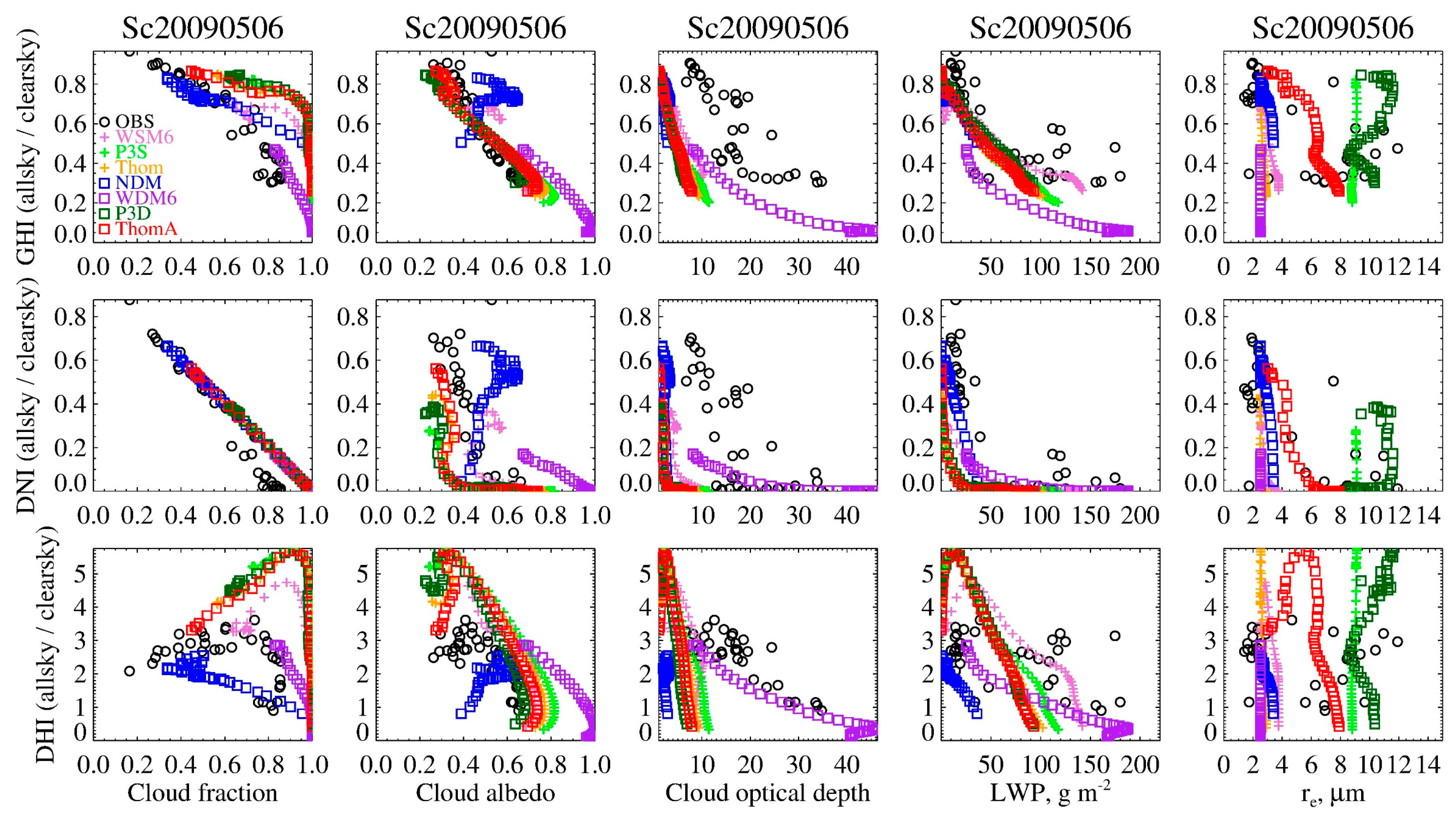
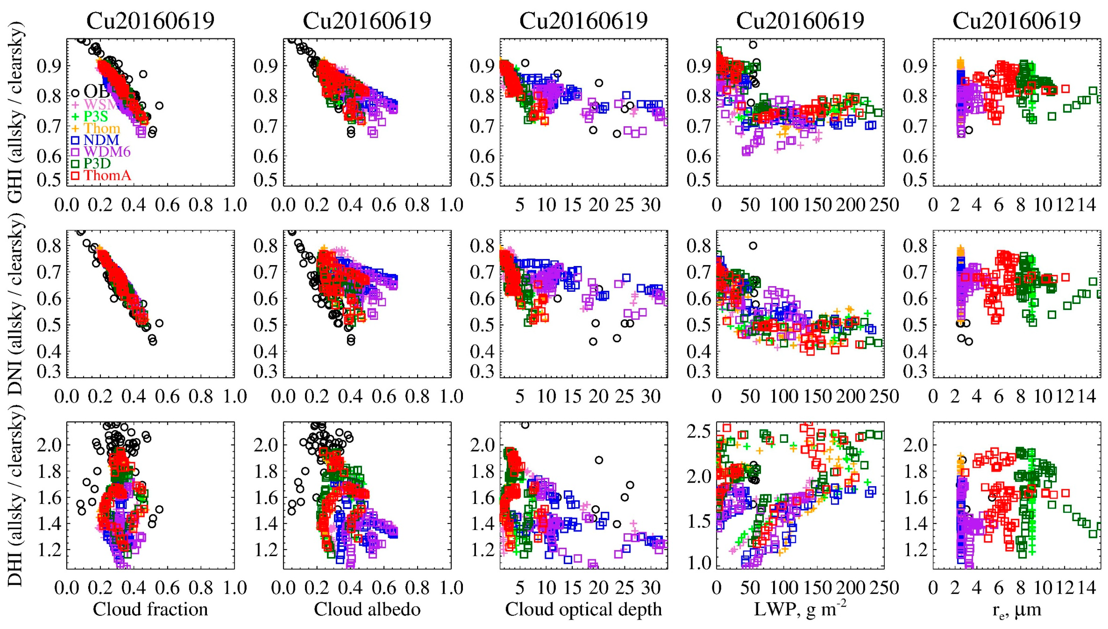
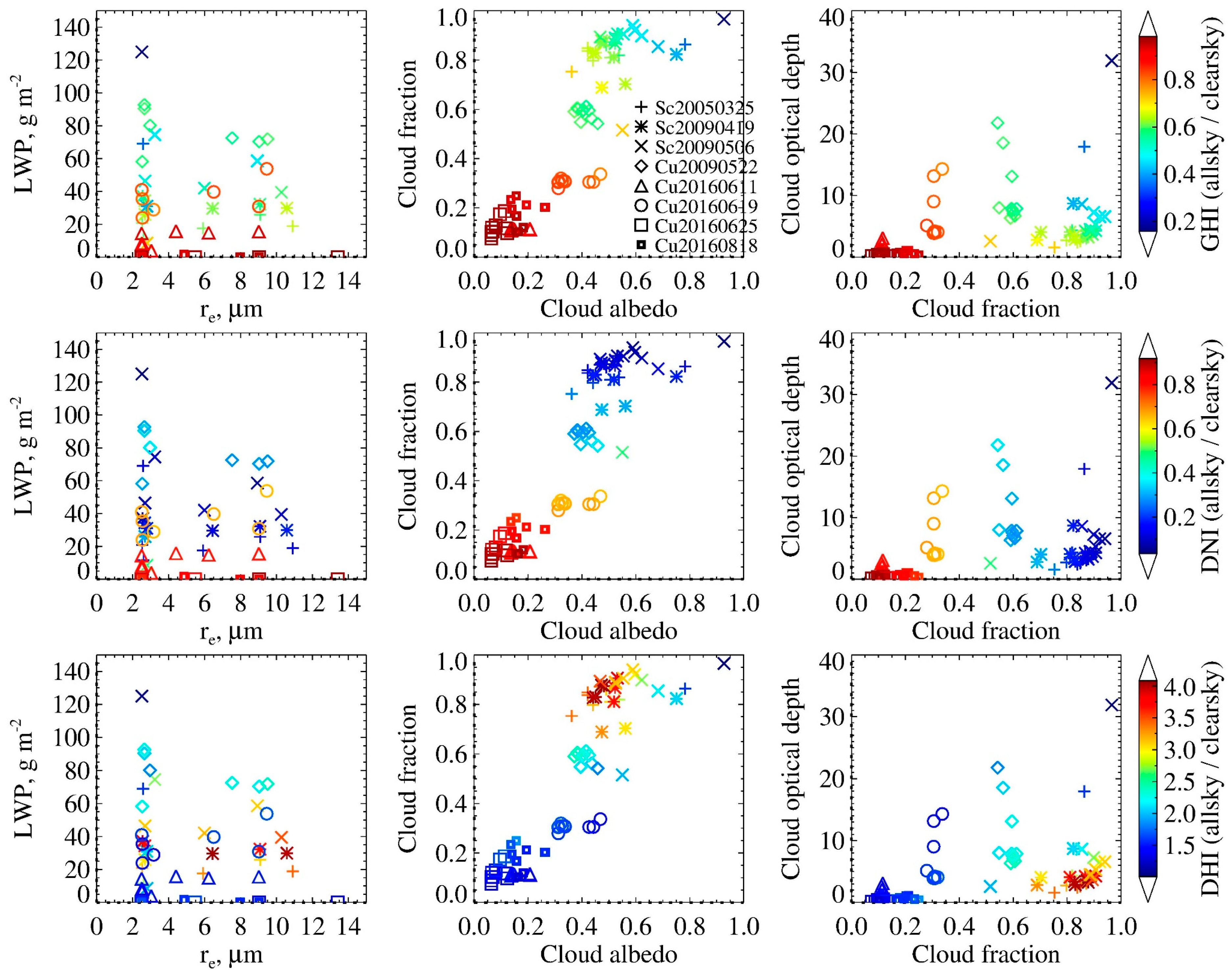
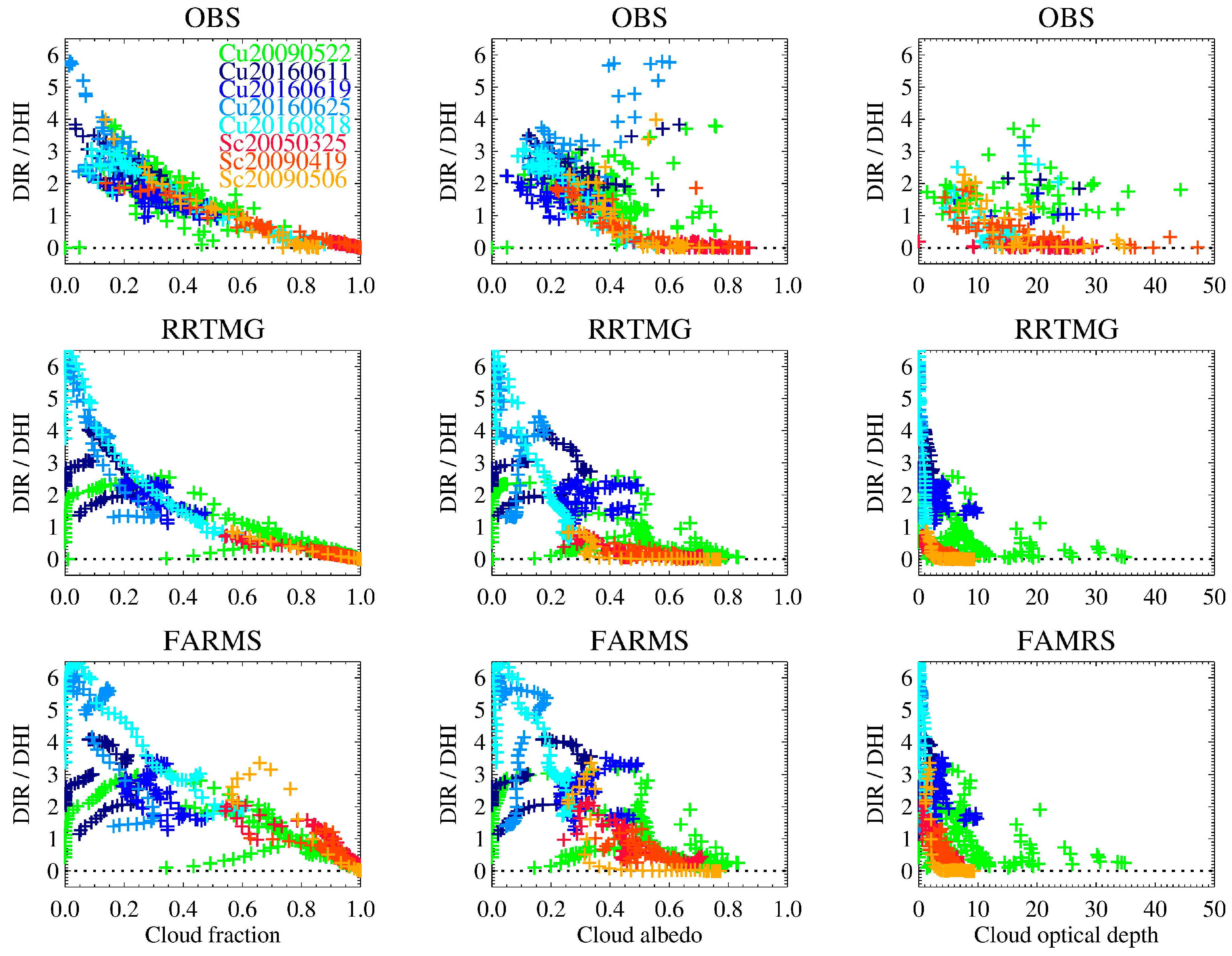
4.3. Influence of Cloud Properties on GHI and Its Partition

The solar irradiance components corresponding to individual cloud properties have been shown in Figure 3, Figure 9 and Figure 10 for different cloudy cases and microphysical schemes. However, the components of solar irradiance are the results of the combined influences of different cloud properties. Figure 11 shows the solar irradiance with the combination of two cloud properties. For the pair of LWP and r e , components of solar irradiance are mainly determined by the LWP. When the LWP is fixed, solar irradiance is enhanced slightly with increasing r e . The pair of cloud fraction and albedo have equivalent influences on solar irradiance. As for the combination of COD and cloud fraction, both cloud properties significantly influence solar irradiance. However, COD has smaller influences on GHI and DNI but a more prominent influence on DHI, likely due to the nonlinear relationship of DHI to cloud properties. The increased cloud fraction leads to increased DHI when COD is small but decreased DHI when COD is large. As a result, the DHI changes more dramatically with COD when the cloud fraction is large. In addition, different microphysical schemes result in similar cloud fractions but more distinct COD in the Cu cases. But, for the Sc cases, different microphysical schemes produce remarkable variations in cloud fraction and COD, which also explains why solar irradiance shows a larger sensitivity in the Sc cases.
One particular feature from the simulated solar irradiance worth highlighting is the compensating errors between DIR and DHI. Figure 12 shows the solar ratio between DIR and DHI with the corresponding cloud properties for all selected cases. In the observation, the solar ratio has negative relations with cloud properties, mainly due to the negative relation between DIR and cloud properties. However, the sensitivity of the solar ratio varies within different ranges of cloud properties. When cloud fraction, albedo, and COD are small, the solar ratio decreases more significantly with increasing cloud properties since DHI is positively related to the clouds under such conditions. When clouds become more abundant and thicker, DHI is attenuated with increasing clouds. Thus, the decrease of solar ratio becomes slower. For cloud albedo and COD, the inflection points are obvious, after which the DIR is close to zero and the solar ratio is almost flat.
In comparison, the RRTMG scheme in WRF-Solar reproduces the negative relations between solar ratio and clouds when the cloud properties are relatively large. However, some simulated Cu cases show a positive relationship between solar ratio and cloud fraction, likely due to the coincidence of the Cu development with the diurnal cycle of solar irradiance. In these cases, Cu initiates in the early morning with small cloud fractions corresponding to small DIR. As time goes on, the cloud fraction increases slowly (so does DHI) while the DIR increases more dramatically as the sun rises, resulting in a positive relationship between the solar ratio and Cu fraction. In other words, the model produces more shallow clouds around dawn and dusk than observations, which leads to the positive relationships in these Cu cases. Besides the response of solar ratio to cloud properties, the biases in the partition of total irradiance are also obvious in the magnitude of the solar ratio. For the simulations with underestimated DIR and overestimated DHI, the solar ratio is smaller than the observations, e.g., Sc20090419, Sc20090506, and Cu20090522 cases. When the DIR is negatively biased, the positive relationship is further enhanced. At the same time, the overestimated DIR and underestimated DHI leads to a solar ratio larger than observation, e.g., Cu20160818. For the current model settings, the biases in the partition of GHI into DIR and DHI are primarily due to the biases in cloud properties. The partition of GHI using another radiative scheme, FARMS, shows similar qualitiave characteristics to RRTMG, that the positive solar ratio is found when the cloud fraction and albedo are small, but the magnitude of solar ratio is different from using the RRTMG scheme in most of the cases.

4.4. Model Uncertainties

Figure 9 and Figure 10 demonstrate how microphysical schemes affect the solar irradiance components through the impacts on r e and LWP. It is expected that any microphysical processes that influence N c , L , and the shape of cloud droplet size distribution, μ , will affect solar irradiance by affecting r e , LWP, and the cloud fraction as well. However, there are many uncertainties in the microphysical schemes used. First of all, the unrealistic uniformed r e is produced by the single-moment schemes with fixed N c and some double-moment schemes without considering the changes in μ . Second, for the double-moment schemes considering the changes in μ , different parameterizations are used for cloud droplet activation and autoconversion, resulting in various N c and L with different microphysical schemes. Third, accurate aerosol input is needed to activate cloud droplets in the double-moment schemes. However, many double-moment schemes do not consider the spatial and temporal variations of aerosols, and the aerosol indirect effect on solar irradiance is not represented in these schemes. Fourth, some processes influencing cloud water are not well-represented in microphysical schemes. For example, the entrainment-mixing is not considered in most microphysical schemes. Also, the relative dispersion of cloud droplets is not well-represented in many processes. Many schemes consider the Kessler-type autoconversion with a sharp change in the threshold function regardless of different cloudy conditions.
In addition, not all the microphysical schemes are fully coupled with radiative schemes to represent the cloud–radiation interaction in the WRF-Solar model. For example, the Morrison, Lin, and NSSL single-moment schemes in WRF V4.1.2 only provide L to the radiative scheme, with the r e prescribed based on temperature and land type information. Thus, these microphysical schemes will have a relatively limited impact on solar irradiance.

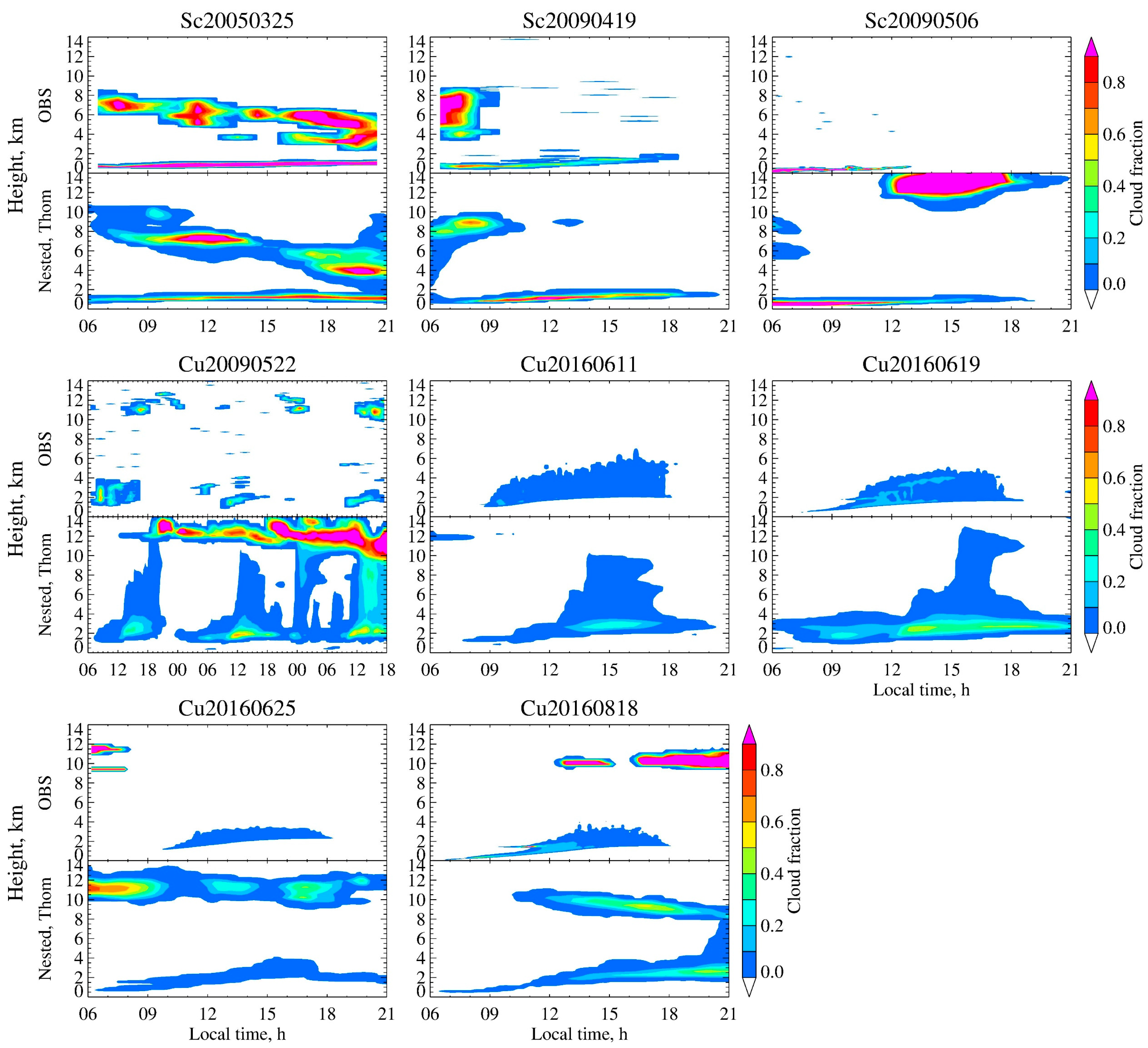
4.5. Vertical Profile of Cloud Fraction

Although the focus of this study is on liquid clouds, the model can generate spurious high clouds (Figure 13). The observed cloud fraction is from the data streams derived from millimeter-wave cloud radar and micropulse lidar at the central facility. WRF-Solar simulations generally capture the observed low-level clouds but with a slight overestimation of cloud fraction and cloud duration in most cases, except for the Sc20050325 case. For example, the Sc20090506 case dissipates about 6 h later in the model, and the simulated Cu cases have a 2–3 h earlier onset and later dissipation compared to the observation. Compared to the fair-weather Cu, the continental Sc has a much thinner cloud depth. It is usually associated with a frontal system, resulting in different environments across the front and stronger synoptic forcing. In the simulations, the deck of Sc is well-captured due to properly represented synoptic-scale forcing. However, the high-level clouds are biased. The coarser vertical resolution at upper levels leads to a diluted cloud fraction with a larger vertical extent in the Sc20050325 case. In addition, the simulations produce a significant amount of fake high clouds, especially in the Cu cases, which is likely a byproduct of the convective parameterizations since no fake high clouds are produced in the corresponding simulations from the Large Eddy Simulation Atmospheric Radiation Measurement Symbiotic Simulation and Observation (LASSO) project [69].
In combination with low clouds, the model-generated high clouds have complex effects on the solar irradiance and present a good example of the possible error compensation between simulated DIR and DHI. Compared to the low clouds, the high clouds are optically thinner. Therefore, slightly overestimated high clouds have a limited impact on DIR, e.g., Cu20160625. However, when the fake high clouds are thick enough, DIR is reduced while DHI is enhanced; the resultant error compensation between DNI and DHR makes GHI less affected, e.g., Sc20090506 around 15:00 LT and Cu20090522 (Figure 2).

5. Conclusions

The influences of cloud microphysics on GHI and its partition into DNI and DHI are examined by use of the WRF-Solar model, with seven different commonly used microphysical parameterizations that are fully coupled with the radiative scheme in WRF Version 4.1.2. Three Sc cases and five Cu cases at the ARM SGP site are examined to represent different cloud types under different weather conditions.
The sensitivities of solar irradiance and cloud properties to microphysical schemes are significant and vary with different cloud types. The solar irradiance in Sc cases have larger sensitivities to microphysical schemes than the Cu cases since Cu has smaller cloud fractions and a domain-averaged total water mixing ratio, thus a limited impact on solar irradiance. When the cloud fraction is similar in Sc cases, larger values of the total water mixing ratio lead to more prominent spreads in simulated solar irradiance with different microphysical schemes. The sensitivity lies in combinations of different LWP and r e , originating from different L , N c , and the shape of cloud droplet distribution produced by the microphysical schemes that further stem from the various treatments of microphysical processes, including cloud droplet nucleation, condensation/evaporation, and autoconversion. Among the examined microphysical schemes, the ThomA scheme has the best performance in terms of both percent error and relative Euclidean distance of the radiative properties, likely due to the better representation of microphysical processes and the consideration of the varying shape of cloud droplet size distribution.
Cloud fraction and cloud albedo have an equally significant impact on solar irradiance, but the responses of individual radiative components are different. Both GHI and DNI are negatively related to cloud fraction and cloud albedo. In contrast, DHI is positively related to cloud fraction and albedo before the clouds are thick enough to attenuate DHI. Furthermore, r e has a smaller influence on COD (thus solar irradiance) than LWP, but it moderates COD when r e is large. The negative relationship between r e and GHI is obvious for given LWP. The partition of GHI also depends on the cloud properties. The errors in the partition are represented as different magnitudes of solar ratio (DIR/DHI), with negatively biased DIR being related to a smaller solar ratio compared to observations and vice versa.
Due to the error cancellation, WRF-Solar simulates GHI better than DNI and DHI. In most cases, the errors in solar irradiance components are closely related to the cloud properties, with overestimated cloud fraction and underestimated cloud optical depth. The overestimated cloud fractions, especially the fake high-level clouds, are likely due to the convection parameterizations used, while the underestimated cloud optical depth is more related to the LWP and r e determined by the microphysical schemes used. Microphysical schemes also exert indirect influences on cloud fraction. Thus, the solar irradiance forecast based on NWP models may benefit more from the ensemble simulations with different parameterizations. In addition, the identified error sources in the physical chain provide crucial insights into future-improving model microphysics.
Several points are noteworthy. First, this study explores the general influences of cloud microphysical parameterization on solar irradiance components and quantifies the spread of uncertainty spanned by seven commonly used schemes. Future studies will focus on specific physical processes, including droplet nucleation, cloud droplet spectral shape representation, autoconversion process, and entrainment-mixing processes. Second, this study uses the WRF-Solar with 3 km horizontal resolution and 100–250 m vertical resolutions near the surface. Similar studies using high-resolution LES simulations that better resolve shallow convection merit future investigation. Third, land types and properties such as surface albedo are expected to affect the numerical simulations as well [70,71,72]. We plan to examine such influences in the future. Finally, clouds and thus the microphysical parameterizations likely exhibit different wavelength dependence [73] beyond the broadband influences on GHI, DNI, and DHI investigated in this study. Thus, detailed spectral dependence merits future investigation.

Author Contributions

Conceptualization, Y.L. and X.Z.; model development, S.E., Y.S. and Y.L.; simulation, X.Z.; formal analysis, X.Z.; investigation, Y.L. and X.Z.; validation, Y.L., X.Z., Y.S., Y.X. and M.S.; resources, Y.L., Y.X. and M.S.; data curation, X.Z.; writing—original draft preparation, X.Z.; writing—review and editing, X.Z. and Y.L.; visualization, X.Z.; supervision, Y.L.; funding acquisition, Y.L. All authors have read and agreed to the published version of the manuscript.

Funding

The work is supported by the US Department of Energy’s Office of Energy Efficiency and Renewable Energy (EERE) under Solar Energy Technologies Office (SETO) award 33504.

Institutional Review Board Statement

Not applicable.

Informed Consent Statement

Not applicable.

Data Availability Statement

The observational datasets are downloaded from the DOE ARM website (https://www.arm.gov/data/). Specifically, RADFLUXANAL is available from https://www.arm.gov/capabilities/science-data-products/vaps/radfluxanal (accessed on 1 October 2023); ARSCL is available from https://www.arm.gov/capabilities/science-data-products/vaps/arscl (accessed on 1 October 2023); MWRRET is available from https://www.arm.gov/capabilities/science-data-products/vaps/mwrret (accessed on 1 October 2023); ARMBE is available from https://www.arm.gov/capabilities/science-data-products/vaps/armbe (accessed on 1 October 2023). The NARR data are available from https://www.ncei.noaa.gov/products/weather-climate-models/north-american-regional (accessed on 1 October 2023). The GEOS-5 product is available from https://www.nccs.nasa.gov/services/data-collections/coupled-products/geos5-forecast (accessed on 1 October 2023). WRF-Solar model used in this study is available from https://github.com/levinzx/wrfsolar_bnl_mp/tree/master/wrfsolar-bnl (accessed on 30 October 2023). The WRF-Solar model simulations presented in this study are available upon request from the corresponding author.

Acknowledgments

The work is supported by the US Department of Energy’s Office of Energy Efficiency and Renewable Energy (EERE) Solar Energy Technologies Office and the Office of Science Atmospheric System Research program. The Brookhaven National Laboratory is operated by the Brookhaven Science Associates, LLC (BSA) for the US Department of Energy under Contract No. DESC0012704. The National Renewable Energy Laboratory is operated by Alliance for Sustainable Energy, LLC, for the US Department of Energy under Contract No. DE-AC36-08GO28308. All computations have been performed on NREL’s Eagle supercomputer.

Conflicts of Interest

The views expressed in the article do not necessarily represent the views of the Department of Energy or the US Government. The US Government retains a nonexclusive, paid-up, irrevocable, worldwide license to publish or reproduce the published form of this work, or allow others to do so, for US Government purposes.

Appendix A. Relationships between Solar Irradiances and Cloud Properties

The effect of clouds on solar irradiance can be quantified by the relative cloud radiative forcing (RCRF) at the surface, α c l d S R F , following Betts and Viterbo [37] as
α c l d S R F = F a l l d n F c l r d n F c l r d n = F a l l d n F c l r d n 1 ,
where F is the surface horizontal irradiance described by a range of superscripts and subscripts, with d n representing downward, a l l representing all sky, and c l r representing a clear sky condition. Liu et al. [38] and Xie and Liu [39] further demonstrate that the RCRF is directly related to the cloud fraction, f , and cloud albedo, α r . Briefly, the downward all sky solar irradiance, F a l l d n , can be expressed by the clear and cloudy component as
F a l l d n = f F c l d d n + 1 f F c l r d n .
Using the single-layer cloud approximation, the cloudy component can be related to the clear component as F c l d d n = ( 1 α r ) ( 1 α a ) F c l r d n , where α a is the cloud aborptance. Thus, Equation (A2) can be rearranged as
F a l l d n F c l r d n 1 = ( α r + α a α r α a ) f .
Since α a is usually much smaller than α r for shortwave radiation, and the second order term α r α a is even smaller, using the definition of α c l d S R F and neglecting the small terms, Equation (A3) can be further simplified to
α c l d S R F = α r f .
Equation (A4) reveals the relationship between solar irradiance and macro cloud properties.
Besides cloud fraction and albedo, the effect of cloud on solar irradiance can also be characterized by the cloud transmittance, T c l d , which is related to cloud optical depth τ c l d by the Beer–Bouguer–Lambert law as
T c l d = exp τ c l d μ 0 ,
where μ 0 is the cosine of the solar zenith angle, and τ c l d is further related to the cloud microphysical and macrophysical properties through the integration of the extinction cross-section of an individual cloud particle over the entire particle size spectrum and the cloud thickness [74,75,76], e.g.,
τ c l d = z = 0 H r = 0 Q e x t π r 2 N ( r ) d r d z ,
in which Q e x t is the efficiency factor for extinction, r is the radius of the cloud particle, N(r) is the number concentration of the cloud particle with size r, z is the height above the cloud base, and H is the cloud thickness. In the radiative scheme, the liquid water clouds are characterized by the liquid water path (LWP), defined as the vertical integral of the liquid water content, L :
L W P = z = 0 H L d z = z = 0 H r = 0 ρ w 4 π 3 r 3 N ( r ) d r d z .
Since the size of cloud droplets (in terms of circumference) is much larger than the wavelengths of solar irradiance, Q e x t approaches the value of 2. Combining the preceding two equations, we obtain
τ c l d = 3 L W P 2 ρ w r e ¯ ,
where r e is the effective radius defined as the ratio between the third and second moment of the droplet size distribution, e.g., r e = 0 r 3 N ( r ) d r / 0 r 2 N ( r ) d r , and r e ¯ denotes the cloud-layer-averaged effective radius. Equation (A8) reveals the second level of the relationship between solar irradiance and cloud microphysical properties.
The relationships between solar irradiance and cloud properties of different levels, e.g., Equations (A4) and (A8), are related using a two-stream approximation with cloud absorptance neglected [77,78],
α r = b τ c l d / μ 0 1 + b τ c l d / μ 0 ,
b = 0.5 0.5 g ,
where g is the asymmetry factor of the cloud particles. Therefore, any influence on LWP and/or r e within the NWP model will affect τ c l d and α r and eventually impact solar irradiance.
From Equation (A2), the downward solar irradiance can be calculated as
F a l l d n = F T O A f T c l d + 1 f T c l e a r ,
where F T O A is the incoming solar irradiance at the top of the atmosphere (TOA), T c l d is the cloud transmittance retrieved from r e and cloud water path, T c l e a r is the transmittance of clear sky. Equation (A11) indicates the way solar irradiance is calculated in the NWP using cloud properties of both levels. Specifically, GHI and DNI are calculated using Equation (A11) with different values of cloud transmittance; then, DIR and DHI are derived from GHI and DNI. And different radiative scheme partitions GHI differently.

Appendix B. Different Microphysical Schemes Used and Their Influences on Shallow Clouds

The influences of shallow clouds on solar irradiances in the NWP models stem from the cloud water content ( L ) and cloud droplet number concentration ( N c ). Spercifically, the two parameters are predicted in the double-moment (DM) bulk microphysical schemes by considering multiple microphysical processes,
L t = ± c o n d e n s a t i o n   o r   e v a p o r a t i o n   a u t o c o n v e r s i o n   t o   r a i n   d r o p s c o l l e c t i o n   b y   r a i n ,   s n o w , g r a u p e l ± m e l t i n g   f r o m   o r   f r e e z i n g   t o   c l o u d   i c e + t u b u l e n t   m i x i n g
and
N c t = + C C N   a c t i v a t i o n ) ( d r o p l e t   e v a p o r a t i o n   a u t o c o n v e r s i o n   t o   r a i n   d r o p s c o l l e c t i o n   b y   r a i n ,   s n o w , g r a u p e l ± m e l t i n g   f r o m   o r   f r e e z i n g   t o   c l o u d   i c e + t u b u l e n t   m i x i n g
Here, we use Thom and ThomA schemes as an example to illustrate how processes in the microphysical schemes impact cloud water and droplet sizes in shallow clouds, thus influencing solar irradiance through the relationships between solar irradiances and different cloud properties. Note that our purpose is to provide physical explanations about the differences in simulated shallow clouds instead of comprehensive details about all the processes in the microphysical schemes used. Thus, only the processes significantly influenced by shallow clouds are highlighted. In the Thom/ThomA schemes, the cloud droplet size distribution is characterized by the Gamma distribution [24,25],
N D = N t Γ ( μ + 1 ) λ μ + 1 D μ e λ D ,
where N t is the total number of cloud particles, D is the particle diameter, λ is the slope of the distribution, μ is the shape parameter representing the width of the distribution, and N D is the particle number with diameter D . Based on the definition of r e , which is the ratio between the third and second moment of droplet size distribution, the above gamma distribution results in an expression used in the scheme to calculate r e as
r e = 0.5 3 + μ λ .
Furthermore, m can also be represented by the cloud droplet relative dispersion ( ε ) defined as the ratio between the standard deviation and mean droplet radius. Many studies have shown that ε is related to N c [27,68,79,80,81,82] and ε = ( μ + 1 ) 1 / 2 by definition using Equation (A14). Based on the observed relationship between ε and N c by Martin et al. [79], Thompson et al. [24] derived an empirical relationship between μ and N c as
μ = min 15 , 10 9 N c + 2 ,
where N c has the unit of m 3 . Although a postive relation between ε and N c (i.e., negative μ ~ N c relation) is used in Thompson schemes, previous studies show that ε is associated with N c in either positive [27,80,82] or negative relations [83].
Equations (A15) and (A16) reveal that the shape of the droplet size distribution will affect the particle sizes for given N c and eventually influence solar irradiance. Compared to the ThomA scheme, all other selected microphysical schemes follows ThomA’s convention to calculate r e by assuming the gamma distribution of cloud droplet similar to Equation (A14), except for the NSSL-DM scheme, which uses a more generalized form of the gamma distribution with four parameters [29,84]. What is more, the treatments of the shape parameter are different among the schemes. For example, WSM6, WDM6 [26], and NDM [29] use constant shape parameters, which are typical for bulk microphysical schemes [85,86]. As for the P3 schemes [28], a variant shape parameter is used, following the same observation of Martin et al. [79] employed in the Thompson schemes.
In the simulation of warm clouds, cloud droplets initiate from CCN activation and grow by the condensation of water vapor. Larger cloud droplets will convert to rain drops through the autoconversion process and fall out of the clouds, while smaller cloud droplets may grow or decrease due to the condensation–evaporation process. In the ThomA scheme, aerosols are divided into the water-friendly aerosol ( N w f a ) and ice-friendly aerosol ( N i f a ), which serve as CCN and ice nuclei (IN), respectively. Cloud droplet nucleation from the water-friendly aerosol ( N w f a ) in ThomA scheme uses a lookup table of an activated fraction based on a parcel model by Feingold and Heymsfield [87], with a given temperature ( T ), vertical velocity ( w ), number of available aerosols ( N w f a ), pre-determined values of the hygroscopicity parameter ( κ = 0.4 ), and mean aerosol radius ( r a = 0.04   μ m ). Specifically, the parcel model follows the widely used power-law between activated cloud droplets and fractional supersaturation ( S ) as [88]
N c = C ( 100 · S ) k ,
where C and k are parameters depending on the air mass type, with typical ranges of C = 30 ~ 300   c m 3 , k = 0.3 ~ 1 for maritime air and C = 300 ~ 3000   c m 3 , k = 0.2 ~ 2 for continental air [89]. And S in the parcel model is resolved by applying the Kohler theory with the five input variables, T , w , N w f a , κ , and r a . In comparison, WDM6 and NDM use a similar empirical relation as Equation (A17) for droplet activation but with different treatments of C , k , and S [26,29]. In the P3-DM scheme, a different relationship is used for droplet activation, which is also based on the explicit treatment of the Kohler theory [27,28].
The autoconversion, which represents the rain initiation from the collision and coalescence of cloud droplets, in the selected schemes are the Kessler-type parameterization [90], which can be represented in a generalized form as [81]:
P L = α a u t o N c 1 3 L 7 3 H D D c ,
where P L is the autoconversion rate of the cloud droplet mass, H ( D D c ) is the Heaviside step function to introduce a threshold of particle size, D c , below which the autoconversion is zero, and α a u t o is a parameter varying with different treatments of collision and coalescence. The autoconversion rate of the droplet number concentration is diagnosed based on P L and the mean volume diameter for the DM schemes. For Thom/ThomA and WDM6, the parameters of autoconversion are derived based on the stochastic collection model by Berry and Reinhardt [91,92]. In comparison, NDM follows the treatments by Ziegler [93], P3 schemes use the relationship proposed by Khairoutdinov and Kogan [32] based on large eddy simulations with bin cloud microphysics, and WSM6 follows the parameterization by Tripoli and Cotton [94]. Note that both N c and L affect autoconversion.
The treatments of the evaporation/condensation of cloud water in the bulk microphysical schemes are based on the supersaturation adjustment, which assumes the cloudy grid is always saturated, and the excess or deficit of water vapor relative to 100% relative humidity will all condensate to, or evaporate from, the cloud droplets over the model time step. For the DM schemes, the completely evaporated cloud droplets return to the CCN category.
Any uncertainties in these microphysical processes will lead to a bias in the simulated solar irradiances. One of the uncertainties lies in the representation of the shape of the cloud droplet spectrum represented by the relative dispersion of cloud droplets, ε . The shape of the droplet size distribution influences the collision and coalescence of the droplets into rain drops and the number of droplets that evaporate in a subsaturated environment. It also determines the droplet sizes in terms of effective radii, r e . However, many microphysical schemes do not consider the influence of the relative dispersion of cloud droplets. The fixed ε regardless of cloud properties and cloud types is not practical.
Based on the preceding processes, solar irradiance in cloudy conditions may be influenced through two pathways known as “aerosol indirect effects”, starting from the changes in the number concentration of aerosols that serve as CCN. First, increasing the aerosol loading increases the cloud droplet concentration and thus decreases r e with other conditions remaining the same, which enhances the cloud optical depth and cloud albedo [95]. Second, the increased cloud droplet number and decreased droplet sizes reduce the efficiency of the autoconversion and accretion processes. As a result, the cloud LWP and duration may increase to reduce solar irradiance at the surface [96]. Note that only the DM schemes can represent the aerosol indirect effect with the prognostic N c in the warm clouds. In comparison, SM schemes with a fixed N c impact the solar irradiance only through the prediction of cloud water. Furthermore, aerosol indirect effects are influenced by ε [68], but the effect of relative dispersion is not well-represented in many microphysical schemes, which is a topic for future study.

References

  1. Marquis, M.; Wilczak, J.; Ahlstrom, M.; Sharp, J.; Stern, A.; Smith, J.C.; Calvert, S. Forecasting the Wind to Reach Significant Penetration Levels of Wind Energy. Bull. Am. Meteorol. Soc. 2011, 92, 1159–1171. [Google Scholar] [CrossRef]
  2. Diagne, M.; David, M.; Lauret, P.; Boland, J.; Schmutz, N. Review of Solar Irradiance Forecasting Methods and a Proposition for Small-Scale Insular Grids. Renew. Sustain. Energy Rev. 2013, 27, 65–76. [Google Scholar] [CrossRef]
  3. Inman, R.H.; Pedro, H.T.C.; Coimbra, C.F.M. Solar Forecasting Methods for Renewable Energy Integration. Prog. Energy Combust. Sci. 2013, 39, 535–576. [Google Scholar] [CrossRef]
  4. Kumar, D.S.; Yagli, G.M.; Kashyap, M.; Srinivasan, D. Solar Irradiance Resource and Forecasting: A Comprehensive Review. IET Renew. Power Gener. 2020, 14, 1641–1656. [Google Scholar] [CrossRef]
  5. Krishnan, N.; Kumar, K.R.; Inda, C.S. How Solar Radiation Forecasting Impacts the Utilization of Solar Energy: A Critical Review. J. Clean. Prod. 2023, 388, 135860. [Google Scholar] [CrossRef]
  6. Perez, R.; Kivalov, S.; Schlemmer, J.; Hemker, K.; Renné, D.; Hoff, T.E. Validation of Short and Medium Term Operational Solar Radiation Forecasts in the US. Sol. Energy 2010, 84, 2161–2172. [Google Scholar] [CrossRef]
  7. Perez, R.; Lorenz, E.; Pelland, S.; Beauharnois, M.; Van Knowe, G.; Hemker, K.; Heinemann, D.; Remund, J.; Müller, S.C.; Traunmüller, W.; et al. Comparison of Numerical Weather Prediction Solar Irradiance Forecasts in the US, Canada and Europe. Sol. Energy 2013, 94, 305–326. [Google Scholar] [CrossRef]
  8. Chen, C.; Duan, S.; Cai, T.; Liu, B. Online 24-h Solar Power Forecasting Based on Weather Type Classification Using Artificial Neural Network. Sol. Energy 2011, 85, 2856–2870. [Google Scholar] [CrossRef]
  9. McCandless, T.C.; Haupt, S.E.; Young, G.S. A Model Tree Approach to Forecasting Solar Irradiance Variability. Sol. Energy 2015, 120, 514–524. [Google Scholar] [CrossRef]
  10. McCandless, T.C.; Haupt, S.E.; Young, G.S. A Regime-Dependent Artificial Neural Network Technique for Short-Range Solar Irradiance Forecasting. Renew. Energy 2016, 89, 351–359. [Google Scholar] [CrossRef]
  11. Hammer, A.; Heinemann, D.; Lorenz, E.; Lückehe, B. Short-Term Forecasting of Solar Radiation: A Statistical Approach Using Satellite Data. Sol. Energy 1999, 67, 139–150. [Google Scholar] [CrossRef]
  12. Descombes, G.; Auligne, D.; Lin, H.-C.; Xu, D.; Schwartz, S.; Vandenberghe, F. Multi-Sensor Advection Diffusion nowCast (MADCast) for Cloud Analysis and Short-Term Prediction. NCAR Tech. Note No NCARTN-509STR 2014. [Google Scholar] [CrossRef]
  13. Jimenez, P.A.; Hacker, J.P.; Dudhia, J.; Haupt, S.E.; Ruiz-Arias, J.A.; Gueymard, C.A.; Thompson, G.; Eidhammer, T.; Deng, A. WRF-Solar: Description and Clear-Sky Assessment of an Augmented NWP Model for Solar Power Prediction. Bull. Am. Meteorol. Soc. 2016, 97, 1249–1264. [Google Scholar] [CrossRef]
  14. Weinstein, L.A.; Loomis, J.; Bhatia, B.; Bierman, D.M.; Wang, E.N.; Chen, G. Concentrating Solar Power. Chem. Rev. 2015, 115, 12797–12838. [Google Scholar] [CrossRef] [PubMed]
  15. Xie, Y.; Sengupta, M.; Liu, Y.; Long, H.; Min, Q.; Liu, W.; Habte, A. A Physics-Based DNI Model Assessing All-Sky Circumsolar Radiation. iScience 2020, 23, 100893. [Google Scholar] [CrossRef] [PubMed]
  16. Smirnov, A.; Holben, B.N.; Eck, T.F.; Slutsker, I.; Chatenet, B.; Pinker, R.T. Diurnal Variability of Aerosol Optical Depth Observed at AERONET (Aerosol Robotic Network) Sites. Geophys. Res. Lett. 2002, 29, 30–31. [Google Scholar] [CrossRef]
  17. Arola, A.; Eck, T.F.; Huttunen, J.; Lehtinen, K.E.J.; Lindfors, A.V.; Myhre, G.; Smirnov, A.; Tripathi, S.N.; Yu, H. Influence of Observed Diurnal Cycles of Aerosol Optical Depth on Aerosol Direct Radiative Effect. Atmos. Chem. Phys. 2013, 13, 7895–7901. [Google Scholar] [CrossRef]
  18. Baklanov, A.; Brunner, D.; Carmichael, G.; Flemming, J.; Freitas, S.; Gauss, M.; Hov, Ø.; Mathur, R.; Schlünzen, K.H.; Seigneur, C.; et al. Key Issues for Seamless Integrated Chemistry–Meteorology Modeling. Bull. Am. Meteorol. Soc. 2017, 98, 2285–2292. [Google Scholar] [CrossRef]
  19. Liu, Y. Introduction to the Special Section on Fast Physics in Climate Models: Parameterization, Evaluation, and Observation. J. Geophys. Res. Atmos. 2019, 124, 8631–8644. [Google Scholar] [CrossRef]
  20. Liu, Y.; Yau, M.-K.; Shima, S.; Lu, C.; Chen, S. Parameterization and Explicit Modeling of Cloud Microphysics: Approaches, Challenges, and Future Directions. Adv. Atmos. Sci. 2023, 40, 747–790. [Google Scholar] [CrossRef]
  21. Baker, M.B. Cloud Microphysics and Climate. Science 1997, 276, 1072–1078. [Google Scholar] [CrossRef]
  22. Khain, A.; Ovtchinnikov, M.; Pinsky, M.; Pokrovsky, A.; Krugliak, H. Notes on the State-of-the-Art Numerical Modeling of Cloud Microphysics. Atmos. Res. 2000, 55, 159–224. [Google Scholar] [CrossRef]
  23. Grabowski, W.W.; Morrison, H.; Shima, S.-I.; Abade, G.C.; Dziekan, P.; Pawlowska, H. Modeling of Cloud Microphysics: Can We Do Better? Bull. Am. Meteorol. Soc. 2019, 100, 655–672. [Google Scholar] [CrossRef]
  24. Thompson, G.; Field, P.R.; Rasmussen, R.M.; Hall, W.D. Explicit Forecasts of Winter Precipitation Using an Improved Bulk Microphysics Scheme. Part II: Implementation of a New Snow Parameterization. Mon. Weather Rev. 2008, 136, 5095–5115. [Google Scholar] [CrossRef]
  25. Thompson, G.; Eidhammer, T. A Study of Aerosol Impacts on Clouds and Precipitation Development in a Large Winter Cyclone. J. Atmos. Sci. 2014, 71, 3636–3658. [Google Scholar] [CrossRef]
  26. Lim, K.-S.S.; Hong, S.-Y. Development of an Effective Double-Moment Cloud Microphysics Scheme with Prognostic Cloud Condensation Nuclei (CCN) for Weather and Climate Models. Mon. Weather Rev. 2009, 138, 1587–1612. [Google Scholar] [CrossRef]
  27. Morrison, H.; Grabowski, W.W. Comparison of Bulk and Bin Warm-Rain Microphysics Models Using a Kinematic Framework. J. Atmos. Sci. 2007, 64, 2839–2861. [Google Scholar] [CrossRef]
  28. Morrison, H.; Milbrandt, J.A. Parameterization of Cloud Microphysics Based on the Prediction of Bulk Ice Particle Properties. Part I: Scheme Description and Idealized Tests. J. Atmos. Sci. 2014, 72, 287–311. [Google Scholar] [CrossRef]
  29. Mansell, E.R.; Ziegler, C.L.; Bruning, E.C. Simulated Electrification of a Small Thunderstorm with Two-Moment Bulk Microphysics. J. Atmos. Sci. 2010, 67, 171–194. [Google Scholar] [CrossRef]
  30. Milbrandt, J.A.; Yau, M.K. A Multimoment Bulk Microphysics Parameterization. Part I: Analysis of the Role of the Spectral Shape Parameter. J. Atmos. Sci. 2005, 62, 3051–3064. [Google Scholar] [CrossRef]
  31. Kogan, Y.L. The Simulation of a Convective Cloud in a 3-D Model With Explicit Microphysics. Part I: Model Description and Sensitivity Experiments. J. Atmos. Sci. 1991, 48, 1160–1189. [Google Scholar] [CrossRef]
  32. Khairoutdinov, M.; Kogan, Y. A New Cloud Physics Parameterization in a Large-Eddy Simulation Model of Marine Stratocumulus. Mon. Weather Rev. 2000, 128, 229–243. [Google Scholar] [CrossRef]
  33. Khain, A.; Pokrovsky, A.; Pinsky, M.; Seifert, A.; Phillips, V. Simulation of Effects of Atmospheric Aerosols on Deep Turbulent Convective Clouds Using a Spectral Microphysics Mixed-Phase Cumulus Cloud Model. Part I: Model Description and Possible Applications. J. Atmos. Sci. 2004, 61, 2963–2982. [Google Scholar] [CrossRef]
  34. Khain, A.P.; Beheng, K.D.; Heymsfield, A.; Korolev, A.; Krichak, S.O.; Levin, Z.; Pinsky, M.; Phillips, V.; Prabhakaran, T.; Teller, A.; et al. Representation of Microphysical Processes in Cloud-Resolving Models: Spectral (Bin) Microphysics versus Bulk Parameterization. Rev. Geophys. 2015, 53, 247–322. [Google Scholar] [CrossRef]
  35. Xue, L.; Fan, J.; Lebo, Z.J.; Wu, W.; Morrison, H.; Grabowski, W.W.; Chu, X.; Geresdi, I.; North, K.; Stenz, R.; et al. Idealized Simulations of a Squall Line from the MC3E Field Campaign Applying Three Bin Microphysics Schemes: Dynamic and Thermodynamic Structure. Mon. Weather Rev. 2017, 145, 4789–4812. [Google Scholar] [CrossRef]
  36. Johnson, J.S.; Cui, Z.; Lee, L.A.; Gosling, J.P.; Blyth, A.M.; Carslaw, K.S. Evaluating Uncertainty in Convective Cloud Microphysics Using Statistical Emulation. J. Adv. Model. Earth Syst. 2015, 7, 162–187. [Google Scholar] [CrossRef]
  37. Betts, A.; Viterbo, P. Land-Surface, Boundary Layer and Cloud-Field Coupling over the South-Western Amazon in ERA-40. J. Geophys. Res. 2005, 110, D14108. [Google Scholar] [CrossRef]
  38. Liu, Y.; Wu, W.; Jensen, M.P.; Toto, T. Relationship between Cloud Radiative Forcing, Cloud Fraction and Cloud Albedo, and New Surface-Based Approach for Determining Cloud Albedo. Atmos. Chem. Phys. 2011, 11, 7155–7170. [Google Scholar] [CrossRef]
  39. Xie, Y.; Liu, Y. A New Approach for Simultaneously Retrieving Cloud Albedo and Cloud Fraction from Surface-Based Shortwave Radiation Measurements. Environ. Res. Lett. 2013, 8, 044023. [Google Scholar] [CrossRef]
  40. Skamarock, C.; Klemp, B.; Dudhia, J.; Gill, O.; Barker, D.; Duda, G.; Huang, X.; Wang, W.; Powers, G. A Description of the Advanced Research WRF Version 3; NCAR Tech. Note NCAR/TN-475+STR; National Center for Atmospheric Research: Boulder, CO, USA, 2008. [Google Scholar] [CrossRef]
  41. Liou, K.-N. On the Absorption, Reflection and Transmission of Solar Radiation in Cloudy Atmospheres. J. Atmos. Sci. 1976, 33, 798–805. [Google Scholar] [CrossRef]
  42. Long, C.N.; Ackerman, T.P. Identification of Clear Skies from Broadband Pyranometer Measurements and Calculation of Downwelling Shortwave Cloud Effects. J. Geophys. Res. Atmos. 2000, 105, 15609–15626. [Google Scholar] [CrossRef]
  43. Long, C.N.; Turner, D.D. A Method for Continuous Estimation of Clear-Sky Downwelling Longwave Radiative Flux Developed Using ARM Surface Measurements. J. Geophys. Res. Atmos. 2008, 113, D18208. [Google Scholar] [CrossRef]
  44. Clothiaux, E.E.; Ackerman, T.P.; Mace, G.G.; Moran, K.P.; Marchand, R.T.; Miller, M.A.; Martner, B.E. Objective Determination of Cloud Heights and Radar Reflectivities Using a Combination of Active Remote Sensors at the ARM CART Sites. J. Appl. Meteorol. Climatol. 2000, 39, 645–665. [Google Scholar] [CrossRef]
  45. Turner, D.D.; Clough, S.A.; Liljegren, J.C.; Clothiaux, E.E.; Cady-Pereira, K.E.; Gaustad, K.L. Retrieving Liquid Wat0er Path and Precipitable Water Vapor From the Atmospheric Radiation Measurement (ARM) Microwave Radiometers. IEEE Trans. Geosci. Remote Sens. 2007, 45, 3680–3690. [Google Scholar] [CrossRef]
  46. Cadeddu, M.P.; Liljegren, J.C.; Turner, D.D. The Atmospheric Radiation Measurement (ARM) Program Network of Microwave Radiometers: Instrumentation, Data, and Retrievals. Atmos. Meas. Tech. 2013, 6, 2359–2372. [Google Scholar] [CrossRef]
  47. Xie, S.; McCoy, R.B.; Klein, S.A.; Cederwall, R.T.; Wiscombe, W.J.; Jensen, M.P.; Johnson, K.L.; Clothiaux, E.E.; Gaustad, K.L.; Long, C.N.; et al. CLOUDS AND MORE: ARM Climate Modeling Best Estimate Data: A New Data Product for Climate Studies. Bull. Am. Meteorol. Soc. 2010, 91, 13–20. [Google Scholar] [CrossRef]
  48. Mesinger, F.; DiMego, G.; Kalnay, E.; Mitchell, K.; Shafran, P.C.; Ebisuzaki, W.; Jović, D.; Woollen, J.; Rogers, E.; Berbery, E.H.; et al. North American Regional Reanalysis. Bull. Am. Meteorol. Soc. 2006, 87, 343–360. [Google Scholar] [CrossRef]
  49. Rienecker, M.M.; Todling, R.; Bacmeister, J.; Takacs, L.; Liu, H.C.; Gu, W.; Sienkiewicz, M.; Koster, R.D.; Gelaro, R.; Stajner, I.; et al. The GEOS-5 Data Assimilation System-Documentation of Versions 5.0.1, 5.1.0, and 5.2.0; Technical Report Series on Global Modeling and Data Assimilation; NASA: Washington, DC, USA, 2008; Volume 27. [Google Scholar]
  50. Lee, J.A.; Haupt, S.E.; Jiménez, P.A.; Rogers, M.A.; Miller, S.D.; McCandless, T.C. Solar Irradiance Nowcasting Case Studies near Sacramento. J. Appl. Meteorol. Climatol. 2016, 56, 85–108. [Google Scholar] [CrossRef]
  51. Haupt, S.E.; Kosović, B.; Jensen, T.; Lazo, J.K.; Lee, J.A.; Jiménez, P.A.; Cowie, J.; Wiener, G.; McCandless, T.C.; Rogers, M.; et al. Building the Sun4Cast System: Improvements in Solar Power Forecasting. Bull. Am. Meteorol. Soc. 2018, 99, 121–136. [Google Scholar] [CrossRef]
  52. Verbois, H.; Huva, R.; Rusydi, A.; Walsh, W. Solar Irradiance Forecasting in the Tropics Using Numerical Weather Prediction and Statistical Learning. Sol. Energy 2018, 162, 265–277. [Google Scholar] [CrossRef]
  53. Ruiz-Arias, J.A.; Dudhia, J.; Gueymard, C.A. A Simple Parameterization of the Short-Wave Aerosol Optical Properties for Surface Direct and Diffuse Irradiances Assessment in a Numerical Weather Model. Geosci. Model Dev. 2014, 7, 1159–1174. [Google Scholar] [CrossRef]
  54. Deng, A.; Gaudet, B.; Dudhia, J.; Alapaty, K. Implementation and Evaluation of a New Shallow Convection Scheme in WRF; American Meteorological Society: Atlanta, GA, USA, 2014. [Google Scholar]
  55. Jimenez, P.A.; Alessandrini, S.; Haupt, S.E.; Deng, A.; Kosovic, B.; Lee, J.A.; Delle Monache, L. The Role of Unresolved Clouds on Short-Range Global Horizontal Irradiance Predictability. Mon. Weather Rev. 2016, 144, 3099–3107. [Google Scholar] [CrossRef]
  56. Xie, Y.; Sengupta, M.; Dudhia, J. A Fast All-Sky Radiation Model for Solar Applications (FARMS): Algorithm and Performance Evaluation. Sol. Energy 2016, 135, 435–445. [Google Scholar] [CrossRef]
  57. Benjamin, S.G.; Weygandt, S.S.; Brown, J.M.; Hu, M.; Alexander, C.R.; Smirnova, T.G.; Olson, J.B.; James, E.P.; Dowell, D.C.; Grell, G.A.; et al. A North American Hourly Assimilation and Model Forecast Cycle: The Rapid Refresh. Mon. Weather Rev. 2016, 144, 1669–1694. [Google Scholar] [CrossRef]
  58. Iacono, M.J.; Delamere, J.S.; Mlawer, E.J.; Shephard, M.W.; Clough, S.A.; Collins, W.D. Radiative Forcing by Long-Lived Greenhouse Gases: Calculations with the AER Radiative Transfer Models. J. Geophys. Res. Atmos. 2008, 113, D13103. [Google Scholar] [CrossRef]
  59. Nakanishi, M.; Niino, H. An Improved Mellor–Yamada Level-3 Model with Condensation Physics: Its Design and Verification. Bound.-Layer Meteorol. 2004, 112, 1–31. [Google Scholar] [CrossRef]
  60. Nakanishi, M.; Niino, H. Development of an Improved Turbulence Closure Model for the Atmospheric Boundary Layer. J. Meteorol. Soc. Jpn. Ser. II 2009, 87, 895–912. [Google Scholar] [CrossRef]
  61. Grell, G.A.; Freitas, S.R. A Scale and Aerosol Aware Stochastic Convective Parameterization for Weather and Air Quality Modeling. Atmos. Chem. Phys. 2014, 14, 5233–5250. [Google Scholar] [CrossRef]
  62. Smirnova, T.G.; Brown, J.M.; Benjamin, S.G.; Kenyon, J.S. Modifications to the Rapid Update Cycle Land Surface Model (RUC LSM) Available in the Weather Research and Forecasting (WRF) Model. Mon. Weather Rev. 2016, 144, 1851–1865. [Google Scholar] [CrossRef]
  63. Olson, J.; Kenyon, J.; Angevine, W.A.; Brown, J.M.; Pagowski, M.; Suselj, K. A Description of the MYNN-EDMF Scheme and the Coupling to Other Components in WRF–ARW; National Oceanic and Atmospheric Administration: Washington, DC, USA, 2019. [Google Scholar]
  64. Xu, K.-M.; Randall, D.A. A Semiempirical Cloudiness Parameterization for Use in Climate Models. J. Atmos. Sci. 1996, 53, 3084–3102. [Google Scholar] [CrossRef]
  65. Hong, S.-Y.; Noh, Y.; Dudhia, J. A New Vertical Diffusion Package with an Explicit Treatment of Entrainment Processes. Mon. Weather Rev. 2006, 134, 2318–2341. [Google Scholar] [CrossRef]
  66. Wu, W.; Liu, Y.; Betts, A.K. Observationally Based Evaluation of NWP Reanalyses in Modeling Cloud Properties over the Southern Great Plains. J. Geophys. Res. Atmos. 2012, 117, D12202. [Google Scholar] [CrossRef]
  67. Liu, Y.; Daum, P.H. Which Size Distribution Function to Use for Studies Related Effective Radius; International Association of Meteorology and Atmospheric Sciences: Reno, NV, USA, 2000; pp. 586–591. [Google Scholar]
  68. Liu, Y.; Daum, P.H. Indirect Warming Effect from Dispersion Forcing. Nature 2002, 419, 580–581. [Google Scholar] [CrossRef] [PubMed]
  69. Gustafson, W.I.; Vogelmann, A.M.; Li, Z.; Cheng, X.; Dumas, K.K.; Endo, S.; Johnson, K.L.; Krishna, B.; Fairless, T.; Xiao, H. The Large-Eddy Simulation (LES) Atmospheric Radiation Measurement (ARM) Symbiotic Simulation and Observation (LASSO) Activity for Continental Shallow Convection. Bull. Am. Meteorol. Soc. 2020, 101, E462–E479. [Google Scholar] [CrossRef]
  70. Varotsos, C.A.; Melnikova, I.N.; Cracknell, A.P.; Tzanis, C.; Vasilyev, A.V. New Spectral Functions of the Near-Ground Albedo Derived from Aircraft Diffraction Spectrometer Observations. Atmos. Chem. Phys. 2014, 14, 6953–6965. [Google Scholar] [CrossRef]
  71. Yang, J.; Li, Z.; Zhai, P.; Zhao, Y.; Gao, X. The Influence of Soil Moisture and Solar Altitude on Surface Spectral Albedo in Arid Area. Environ. Res. Lett. 2020, 15, 035010. [Google Scholar] [CrossRef]
  72. Aoki, T.; Aoki, T.; Fukabori, M.; Hachikubo, A.; Tachibana, Y.; Nishio, F. Effects of Snow Physical Parameters on Spectral Albedo and Bidirectional Reflectance of Snow Surface. J. Geophys. Res. Atmos. 2000, 105, 10219–10236. [Google Scholar] [CrossRef]
  73. Melnikova, I.; Simakina, T.; Vasilyev, A.; Gatebe, C.; Varotsos, C. Does Scattered Radiation Undergo Bluing within Clouds? AIP Conf. Proc. 2013, 1531, 171–175. [Google Scholar] [CrossRef]
  74. Liou, K.N. An Introduction to Atmospheric Radiation, 2nd ed.; Academic Press: Amsterdam, The Netherlands; Boston, MA, USA, 2002; ISBN 978-0-12-451451-5. [Google Scholar]
  75. Stephens, G.L. Radiation Profiles in Extended Water Clouds. II: Parameterization Schemes. J. Atmos. Sci. 1978, 35, 2123–2132. [Google Scholar] [CrossRef]
  76. Brenguier, J.-L.; Burnet, F.; Geoffroy, O. Cloud Optical Thickness and Liquid Water Path–Does the k Coefficient Vary with Droplet Concentration? Atmos. Chem. Phys. 2011, 11, 9771–9786. [Google Scholar] [CrossRef]
  77. Sagan, C.; Pollack, J.B. Anisotropic Nonconservative Scattering and the Clouds of Venus. J. Geophys. Res. 1896-1977 1967, 72, 469–477. [Google Scholar] [CrossRef]
  78. Meador, W.E.; Weaver, W.R. Two-Stream Approximations to Radiative Transfer in Planetary Atmospheres: A Unified Description of Existing Methods and a New Improvement. J. Atmos. Sci. 1980, 37, 630–643. [Google Scholar] [CrossRef]
  79. Martin, G.M.; Johnson, D.W.; Spice, A. The Measurement and Parameterization of Effective Radius of Droplets in Warm Stratocumulus Clouds. J. Atmos. Sci. 1994, 51, 1823–1842. [Google Scholar] [CrossRef]
  80. Grabowski, W.W. Toward Cloud Resolving Modeling of Large-Scale Tropical Circulations: A Simple Cloud Microphysics Parameterization. J. Atmos. Sci. 1998, 55, 3283–3298. [Google Scholar] [CrossRef]
  81. Liu, Y.; Daum, P.H. Parameterization of the Autoconversion Process.Part I: Analytical Formulation of the Kessler-Type Parameterizations. J. Atmos. Sci. 2004, 61, 1539–1548. [Google Scholar] [CrossRef]
  82. Rotstayn, L.D.; Liu, Y. Sensitivity of the First Indirect Aerosol Effect to an Increase of Cloud Droplet Spectral Dispersion with Droplet Number Concentration. J. Clim. 2003, 16, 3476–3481. [Google Scholar] [CrossRef]
  83. Wang, J.; Daum, P.H.; Yum, S.S.; Liu, Y.; Senum, G.I.; Lu, M.-L.; Seinfeld, J.H.; Jonsson, H. Observations of Marine Stratocumulus Microphysics and Implications for Processes Controlling Droplet Spectra: Results from the Marine Stratus/Stratocumulus Experiment. J. Geophys. Res. Atmos. 2009, 114. [Google Scholar] [CrossRef]
  84. Seifert, A.; Beheng, K.D. A Two-Moment Cloud Microphysics Parameterization for Mixed-Phase Clouds. Part 1: Model Description. Meteorol. Atmos. Phys. 2006, 92, 45–66. [Google Scholar] [CrossRef]
  85. Ferrier, B.S. A Double-Moment Multiple-Phase Four-Class Bulk Ice Scheme. Part I: Description. J. Atmos. Sci. 1994, 51, 249–280. [Google Scholar] [CrossRef]
  86. Girard, E.; Curry, J.A. Simulation of Arctic Low-Level Clouds Observed during the FIRE Arctic Clouds Experiment Using a New Bulk Microphysics Scheme. J. Geophys. Res. Atmos. 2001, 106, 15139–15154. [Google Scholar] [CrossRef]
  87. Feingold, G.; Heymsfield, A.J. Parameterizations of Condensational Growth of Droplets for Use in General Circulation Models. J. Atmos. Sci. 1992, 49, 2325–2342. [Google Scholar] [CrossRef]
  88. Twomey, S. The Nuclei of Natural Cloud Formation Part II: The Supersaturation in Natural Clouds and the Variation of Cloud Droplet Concentration. Geofis. Pura E Appl. 1959, 43, 243–249. [Google Scholar] [CrossRef]
  89. Yau, M.K.; Rogers, R.R. A Short Course in Cloud Physics; Elsevier: Amsterdam, The Netherlands, 1996; ISBN 978-0-08-057094-5. [Google Scholar]
  90. Kessler, E. On the Distribution and Continuity of Water Substance in Atmospheric Circulations; Meteorological Monographs; American Meteorological Society: Boston, MA, USA, 1969; pp. 1–84. [Google Scholar]
  91. Berry, E.X.; Reinhardt, R.L. An Analysis of Cloud Drop Growth by Collection: Part I. Double Distributions. J. Atmos. Sci. 1974, 31, 1814–1824. [Google Scholar] [CrossRef]
  92. Berry, E.X.; Reinhardt, R.L. An Analysis of Cloud Drop Growth by Collection Part II. Single Initial Distributions. J. Atmos. Sci. 1974, 31, 1825–1831. [Google Scholar] [CrossRef]
  93. Ziegler, C.L. Retrieval of Thermal and Microphysical Variables in Observed Convective Storms. Part 1: Model Development and Preliminary Testing. J. Atmos. Sci. 1985, 42, 1487–1509. [Google Scholar] [CrossRef]
  94. Tripoli, G.J.; Cotton, W.R. A Numerical Investigation of Several Factors Contributing to the Observed Variable Intensity of Deep Convection over South Florida. J. Appl. Meteorol. Climatol. 1980, 19, 1037–1063. [Google Scholar] [CrossRef]
  95. Twomey, S. Pollution and the Planetary Albedo. Atmos. Environ. 1967 1974, 8, 1251–1256. [Google Scholar] [CrossRef]
  96. Albrecht, B.A. Aerosols, Cloud Microphysics, and Fractional Cloudiness. Science 1989, 245, 1227–1230. [Google Scholar] [CrossRef]
Figure 1. WRF-Solar domains and locations of ARM SGP facilities with solar irradiance measurements (RADFLUXANAL). Purple-colored sites have data available for cases in 2009 and earlier, while black-colored sites have data available for 2016, and the sites with two colors overlapped are available at both periods. Most of the data streams are available at the central facility, C1 for all cloudy cases. The green box indicates the nested WRF-Solar inner domain at a 3 km horizontal grid resolution (90 km × 90 km). Solar irradiance measurements are averaged within the red circle (130 km radius centered on C1), and cloud measurements at C1 are compared to the domain-averaged model simulations.
Atmosphere 15 00039 g001
Figure 2. Temporal changes of solar irradiances for different cases. The first–fourth columns are for the GHI, DIR, DHI, and DNI, respectively. Each case is represented in a row. The observation is spatially averaged within the red circle (130 km radius) in Figure 1 to keep a large enough sample size while being close to the central facility. The simulated solar irradiances are the averages over the inner model domain. The simulations shown are conducted with the default Thom cloud microphysical scheme.
Atmosphere 15 00039 g002
Figure 3. Relationships between the errors in macrophysical cloud properties and errors in solar irradiances during the observed cloudy periods for all the cases using the Thom microphysical scheme. The percent errors in GHI, DNI, and DHI are shown in the first–third columns. The cloud fraction, cloud albedo, and COD are shown in the first–third rows, respectively. The errors in solar irradiance are normalized to the observation to minimize the influence of a strong diurnal cycle; thus, the percent errors in DNI and DIR are identical. The cloud fraction and cloud albedo shown here are derived from GHI and DIR and the corresponding clear-sky values with the approach presented in [38,39] (see Appendix A).
Atmosphere 15 00039 g003
Figure 4. Relationships between the errors among r e , LWP, and COD using the Thom microphysical scheme for all cloudy cases. The errors in COD are colored corresponding to the combination of given errors in r e and LWP.
Atmosphere 15 00039 g004
Figure 5. The range of difference in simulated solar irradiances measured as the maximum and minimum resulting from different microphysical schemes. The first row shows the relative maximum (solid) and minimum (dotted) deviations from of the ensemble means of GHI, DNI, and DHI. The second row shows the absolute differences in solar irradiances between the maximum and minimum values. Only the observed cloudy periods are shown. The Cu20090522 case is excluded because of its different temporal length.
Atmosphere 15 00039 g005
Figure 6. Dispersion (standard deviation/ensemble mean) in solar irradiance using different microphysical schemes against the ensemble mean of the total cloud water mixing ratio (cloud water + ice) weighted by the vertical depth of cloudy grids (e.g., cloud water path divided by cloud thickness). All properties are domainaveraged temporal values.
Atmosphere 15 00039 g006
Figure 7. Same as Figure 5 but for the range of differences in cloud properties, including cloud fraction, cloud albedo, COD, LWP, re, qc, and Nc. Cloud properties shown have more and more direct influence by the microphysical scheme from the top row to the bottom row.
Atmosphere 15 00039 g007
Figure 8. Evaluation metrics on solar irradiance and cloud properties using different microphysical schemes. Sc20090506 and Cu20160619 cases are shown in the first and second columns; the percent error, relative Euclidean distance, and the individual contribution from the mean, standard deviation, and correlation are shown in different rows.
Atmosphere 15 00039 g008
Figure 9. Relationships between solar irradiances and various cloud properties for the Sc20090506 case simulated by WRF-Solar, with different microphysical schemes colored using the crosses, representing single-moment schemes, and squares, representing double-moment schemes. All properties are spatially averaged over all available stations for observation (e.g., in the red cycle of Figure 1 for the solar irradiances and C1 facility for cloud properties) and the entire inner model domain for simulations including cloud-free columns, except for r e , which is a cloud-scale average. The normalized solar irradiances (allsky/clearsky) are used to minimize the effect of the solar diurnal cycle, and the normalized DNI and DIR are identical.
Atmosphere 15 00039 g009
Figure 10. Same as Figure 9 but for the Cu20160619 case.
Atmosphere 15 00039 g010
Figure 11. Solar irradiances as a joint function of two cloud properties. Each point represents the spatial and temporal average of a simulated case during observed cloudy hours. Different cloudy cases are represented with different symbols, and the group of the same symbol represents various microphysical schemes used for the specific case.
Atmosphere 15 00039 g011
Figure 12. The partition of GHI in terms of solar ratio (DIR/DHI) with different cloud properties for all cases using the ThomA scheme. All properties are spatially averaged for the observed cloudy periods.
Atmosphere 15 00039 g012
Figure 13. Temporal variation of vertical profiles of the cloud fraction of all selected cases. Each cloudy case is represented in a separate panel, with the upper half showing the observation at the central facility and lower half showing the simulation using the default physics package with the Thom microphysical scheme.
Atmosphere 15 00039 g013
Table 1. Selected cloudy cases for the WRF-Solar simulations. The name consists of cloud type (Cu or Sc) and starting date of the case (yyyymmdd). Case duration is the period of simulation in local time instead of the exact duration of the clouds. The evaluation is focused on the period when low-level cloud persists.
Name (Type & Date) Cloud ConditionCase Duration
Sc20050325Low-level and mid-level stratocumulus15 h from 6:00
Sc20090419Single-layer low-level stratocumulus15 h from 6:00
Sc20090506Single-layer low-level stratocumulus15 h from 6:00
Cu20090522Shallow cumulus with high-level ice clouds60 h from May 22 6:00
Cu20160611Shallow cumulus15 h from 6:00
Cu20160619Shallow cumulus15 h from 6:00
Cu20160625Shallow cumulus15 h from 6:00
Cu20160818Shallow cumulus with high-level ice clouds15 h from 6:00
Table 2. Model configuration and the microphysical schemes examined.
ConfigurationsDescriptions
InputsNARRInitial and boundary conditions
GEOS-5Aerosol optical properties
*# of domains2
*# of vertical levels50Decrease linearly in pressure
Grid resolution3 kmInner domain
MicrophysicsThompson (Thom **)mp_phsyics option = 8
Thompson aerosol aware (ThomA **)mp_phsyics option = 28
WSM6mp_phsyics option = 6
WDM6mp_phsyics option = 16
NSSL double-moment (NDM **)mp_phsyics option = 17
P3 single-moment (P3S **)mp_phsyics option = 50
P3 double-moment (P3D **)mp_phsyics option = 52
RadiationRRTMG
Boundary layer and shallow convectionMYNN-EDMF
Land surfaceRUC
Deep ConvectionGrell–Freitas, (GF)
*# means number; ** Short notation for microphysics scheme used in this study.
Disclaimer/Publisher’s Note: The statements, opinions and data contained in all publications are solely those of the individual author(s) and contributor(s) and not of MDPI and/or the editor(s). MDPI and/or the editor(s) disclaim responsibility for any injury to people or property resulting from any ideas, methods, instructions or products referred to in the content.

