Article

Mapping Prediction of Surface Solar Radiation with Linear Regression Models: Case Study over Reunion Island

1
Guangxi University of Science and Technology, 2 Avenue Wenchang, Chengzhong District, Liuzhou 545006, China
2
ENERGY-Lab, University of La Réunion, 15, Avenue René Cassin CS 92003, CEDEX 9, 97744 Saint-Denis, France
*
Authors to whom correspondence should be addressed.
Atmosphere 2023, 14(9), 1331; https://doi.org/10.3390/atmos14091331
Submission received: 22 July 2023 / Revised: 14 August 2023 / Accepted: 15 August 2023 / Published: 23 August 2023

Abstract

:
This paper presents a novel mapping prediction method for surface solar radiation with linear regression models. The dataset for surface solar radiation prediction is the daily surface incoming shortwave radiation (SIS) product from CM SAF SARAH-E. The spatial resolution is 0.05° × 0.05° and the temporal coverage is from 2007 to 2016. The first five years (2007–2011) are used as training data, and the remaining five years (2012–2016) are used as test data in the prediction model. Datasets were detrended, de-seasonalized, and normalized before being applied to multiple linear regression (MLR), principal component regression (PCR), stepwise regression (SR), and partial least squares regression (PLSR), which are used to perform prediction mapping. The statistical analysis using MAE, MSE, and RMSE shows that the PCR model had the smallest MAE, MSE, and RMSE as compared to the other three models. The PCR model seems better for SSR mapping prediction over Reunion Island. Although the PCR model provides better prediction results, its MAE, MSE, and RMSE are quite large.

1. Introduction

Reunion Island is a French overseas territory that lies at 21°06′ South and 55°32′ East. Figure 1 shows the global horizontal irradiance (GHI) (kWh/m2) distribution on Reunion Island [1]. The annual sunshine on Reunion Island is in the range of 1400–2500 h and can reach a value of 2900 h at altitudes lower than 400 m. The monthly daily radiation reaches more than 6.5 kWh/m2 during the austral summer season in some parts of the coastal region (altitude < 300 m). Daily insulation is characterized by a strong evolution due to orographic cloud formations on the mountains. The two main applications of solar energy in Reunion are solar water heating and photovoltaic electricity (PV). And Reunion is actively engaged in the development and promotion of solar thermal and PV energy through various action plans and programs in the context of sustainable development, such as GERRI, PRERURE, and so on, because of its solar energy potential [2].
Before making use of the abundant solar energy for electricity generation, it is necessary to evaluate and predict how much surface solar radiation we could obtain, especially given the complex geography and few ground observation stations over Reunion Island [3]. There were many different solar energy forecasting methods applied in previous studies. Gueymard evaluated the performance of broadband direct irradiance predictions through investigation of nineteen models selected from a literature survey [4]. According to [5], Boata and Pop used Takagi-Sugeno fuzzy algorithms to estimate daily global solar irradiation with the station data of Timisoara. Calinoiu et al. proposed a clear-sky solar irradiance mode based on atmospheric parameters at five stations [6]. Either those studies focused on numerical weather prediction methods or they used ground-based or satellite image techniques. More and more researchers are conducting deep learning to predict surface solar radiation or its direct/diffuse parts [7].Oyewola et al. [8] made a global solar radiation prediction for the Fiji Islands based on empirical models. Bamisile et al. compared machine learning and deep learning algorithms for hourly global/diffuse solar radiation predictions and applied these models to four different locations in Nigeria [9]. An evolutionary robust solar radiation prediction model based on WT-CEMDAN (wavelet transform and complete ensemble empirical mode decomposition with adaptive noise) and IASO-optimized (improved atom search optimization) outlier robust extreme learning machines was proposed by Zhang et al. [10]. A hybrid deep learning CNN-REGST method where a convolutional neural network was integrated with a dual-stage stacked regression followed by a support vector machine to predict the daily global solar radiation was proposed by Ghimire et al., and this model was tested on six solar energy farms in Queensland, Australia [11]. An artificial neural network (ANN) and a recurrent neural network (RNN) model were developed in the Pang et al. study to investigate the performances of the deep learning algorithms for the solar radiation prediction [12]. Samuel et al. provided a statistical analysis of the efficiency of real-time solar systems simulated numerically and probabilistically as a renowned approach for beam, diffuse, and global solar radiation prediction in Southern African and Middle Eastern countries [13]. The studies above mostly predicted one or a few of the stations’ surface solar radiation but did not focus on an “area”. Those studies mostly had enough observational data, or the study area was not overly complex. And their prediction results could not present a big picture of the surface solar radiation’s distribution.
There have been some studies on solar radiation forecasting that have also focused on Reunion Island. Diagne et al. used a weather research and forecasting (WRF) model to forecast day-ahead solar radiation in one year covering Reunion Island [14]. Boata et al. used numerical weather prediction with thermodynamic variables as predictors to forecast the solar radiation over Reunion Island [5]. Lauret et al. proposed a benchmarking of supervised machine learning techniques to forecast the global horizontal solar irradiance [15]. Li et al. conducted the prediction of daily surface solar radiation maps for Reunion Island via a hybrid approach that combines principal component analysis, wavelet transform analysis, and ANN [16,17]. In this study, a novel mapping prediction method of surface solar radiation with linear regression models is proposed over Reunion Island. This method could be seen as another test of mapping prediction like [16,17].
This paper is organized as follows: Section 2 describes the surface solar radiation dataset used in this study and the methodology of the 1-day-ahead SSR mapping prediction. Section 3 presents the results of data pre-processing. Section 4 is dedicated to the presentation and discussion of the prediction results, which are then briefly summarized in Section 5.

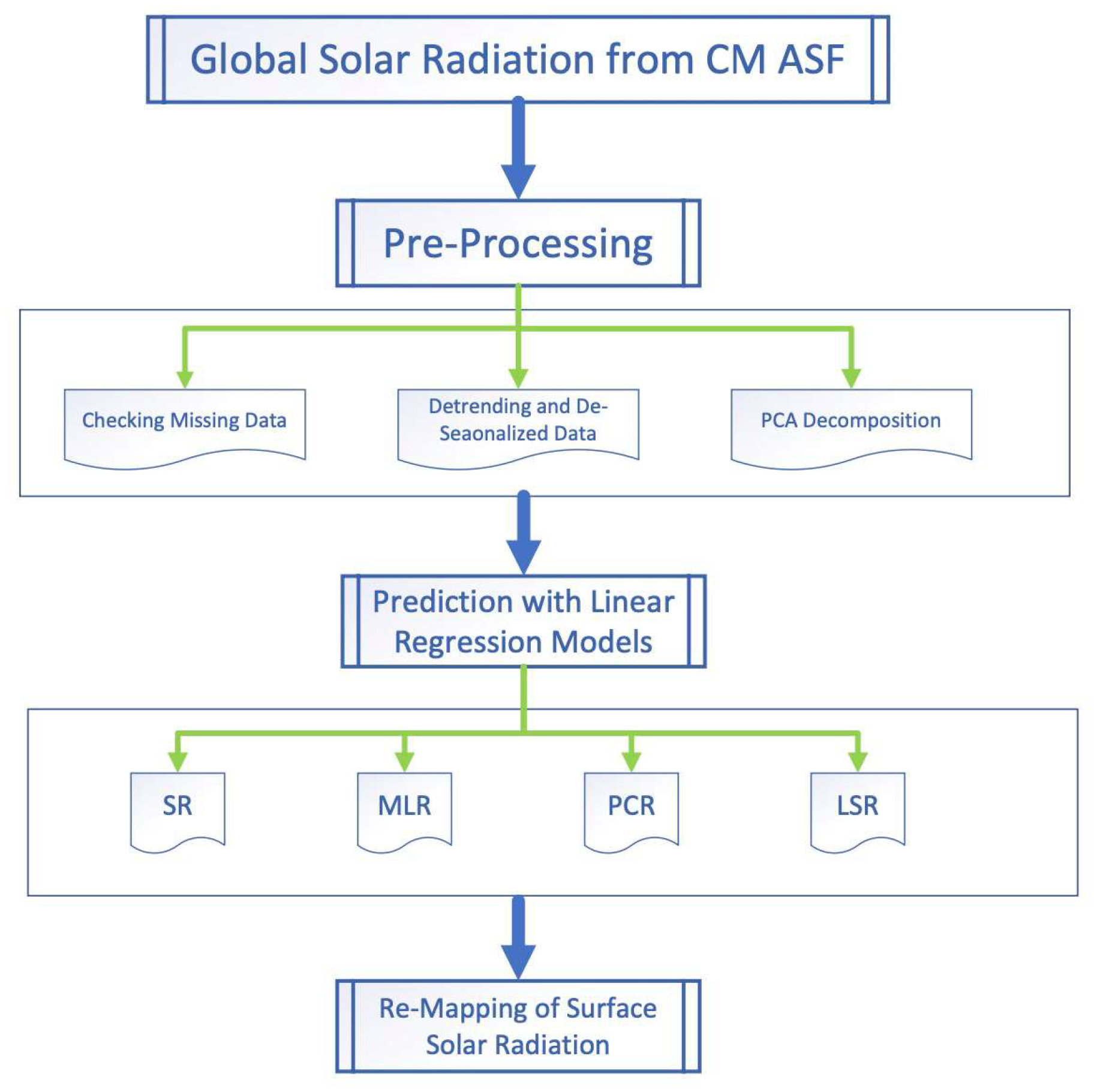
2. Dataset and Methodology

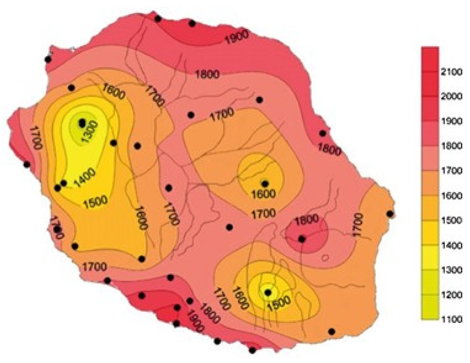
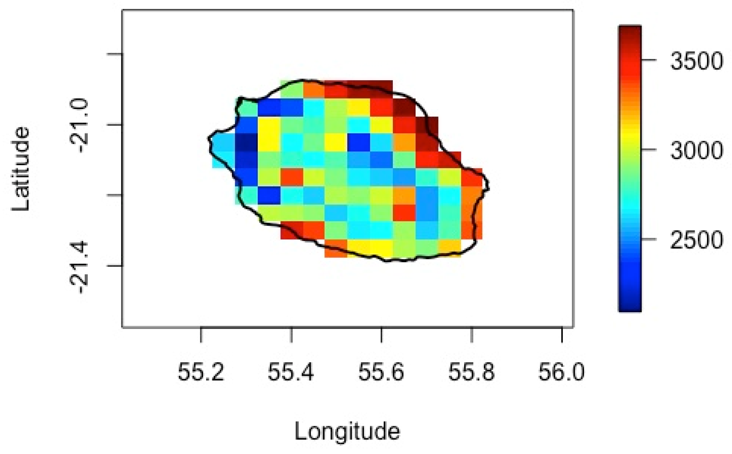
2.1. Global Solar Radiation from CM SAF

The dataset for surface solar radiation prediction is the daily surface incoming shortwave radiation (SIS) product from CM SAF surface solar radiation data records for Heliosat-East (SARAH-E), which are based on observations from the METEOSAT-East satellites [18]. The spatial resolution is 0.05° × 0.05°, and the temporal coverage is from 2007 to 2016. The mean of absolute bias (standard deviation) against reference ground measurements of the Baseline Surface Radiation Network for the daily mean of SIS is 15.3 (21.1) W/m2 [19]. In this study, the first five years (2007–2011) were used as training data, and the remaining five years (2012–2016) were used as test data in the prediction model.

2.2. Methodology for the 1-Day-Ahead SSR Mapping Prediction

There are many studies on the SSR prediction model that are based on one-site time series prediction (univariate or multivariate model). The goal of the present work is to build a spatio-temporal multivariate model for mapping prediction. Each pixel of the Reunion map could be predicted. Therefore, our new concept for 1-day-ahead SSR prediction was to combine spatial and temporal correlation for building a set of daily maps using SSR daily satellite data (CM SAF@5 km). As the 10 years (2007–2016) of SIS data were used for the prediction, the first step was to conduct data pre-processing, which included checking the missing data, detrended and de-seasonalized data, and principle component analysis (PCA) decomposition. Then, the PC was used as input to conduct predictions using the four linear regression models: multiple linear regression (MLR), principal component regression (PCR), stepwise regression (SR), and partial least squares regression (PLSR). In the end, the predicted SIS could be obtained, and the re-mapping of the distribution SIS could directly show the performance of the prediction models. The methodology is presented in the flowchart in Figure 2.
In this study, multiple linear regression (MLR), principal component regression (PCR), stepwise regression (SR), and partial least squares regression (PLSR) are used to perform prediction mapping, which are described in the following briefly:
(1)
Multiple Linear Regression (MLR)
In simple linear regression, a single predictor variable X is used to model the response variable Y. However, in many applications, there is more than one factor that influences the response. MLR models thus describe how a single response variable Y depends linearly on a number of predictor variables. A MLR model with k predictor variables X1, X2, …, Xk and a response Y can be written as:
y = β 0 + β 1 x 1 + β 2 x 2 + β k x k + ϵ
where β0, β1, β2, , βk are coefficients and ϵ is the residual term of the model.
The MLR could be thought of as an extension of simple linear regression.
(2)
Principal Component Regression (PCR)
PCR is a technique for analyzing multiple regression data that suffers from multicollinearity. In PCR, a principal component analysis (PCA) is conducted on the design matrix, and then the first k principal components are used to conduct the regression.
(3)
Stepwise Regression (SR)
Stepwise regression is an automated tool used in the exploratory stages of model building in order to identify a useful subset of predictors. In each step, a variable is considered for addition to or subtraction from the set of explanatory variables based on some prespecified criterion. The main approaches include: (1) forward selection, which involves starting with no variables in the model, testing the addition of each variable using a chosen model fit criterion, adding the variable whose inclusion provides the most statistically significant improvement of the fit, and repeating this process until none improves the model to a statistically significant extent; (2) backward elimination, which involves starting with all candidate variables, testing the deletion of each variable using a chosen model fit criterion, deleting the variable whose loss provides the most statistically insignificant deterioration of the model fit, and repeating this process until no further variables can be deleted without a statistically significant loss of fit; and (3) bidirectional elimination, a combination of the above, testing at each step for variables to be included or excluded.
(4)
Partial Least Squares Regression (PLSR)
PLSR is a powerful and frequently applied technique used in multivariate statistical process control when the process variables are highly correlated. It is a technique that reduces the predictors to a smaller set of uncorrelated components and performs least squares regression on these components instead of on the original data. PLSR is especially useful when the predictors are highly collinear or when there are more predictors than observations, and ordinary least-squares regression either produces coefficients with high standard errors or fails completely. PLSR does not assume that the predictors are fixed, unlike MLR. This means that the predictors can be measured with error, making PLSR more robust to measurement uncertainty.
A regression model needs a set of predictors and predictands, as we know. In this study, the satellite data used to perform prediction is from SARAH-E (CM SAF @5 km), which covers Reunion Island with 360 pixels. In this sense, there is a large set of predictors and predictands. Building a prediction model with satellite data is not easy when the number of variables increases. It would require a large amount of CPU time to perform the regression process. Finding a way to reduce the size of the dimension set of the variables could be the first step in the analysis. There are many methods of dimension reduction. Some of these are principal component analysis (PCA), canonical correlation analysis (CCA), kernel PCA, and k-nearest neighbor (k-NN) [20]. PCA is commonly used in climate research as a tool to analyze meteorological fields with high spatio-temporal dimensionality. PCA aims at finding a new set of variables that captures most of the observed variance from the data through a linear combination of the original variables [21,22,23]. In this paper, PCA was chosen to conduct the dimension reduction.

3. Data Pre-Processing

3.1. Checking the Missing Data

The SARAH-E satellite data (CM SAF) were used to perform the 1-day-ahead prediction for surface solar radiation (SSR) over Reunion Island. The domain used for the prediction was 55.05 E~56 E, −21.55 S~−20.70 S, which covers Reunion Island, as shown in Figure 3. Because the 10 years of data were from satellite and there were not many missing days, the days for which we did not have records have been removed.
From Figure 4a,c,e,h, the obvious seasonal variability can be observed. The austral summer season (DJF: December–January–February) obtains more SSR than the austral winter season (JJA: June–July–August) over the whole island. During the inter-season (MAM: March–April–May and SON: September–October–November), there is more SSR over the northeast coast than over the inland area because, in this period, strong thermal and wind inversion occurs [24]. Turbulent flow and cloud activities over the island are thus exclusively vertical in the boundary layer.

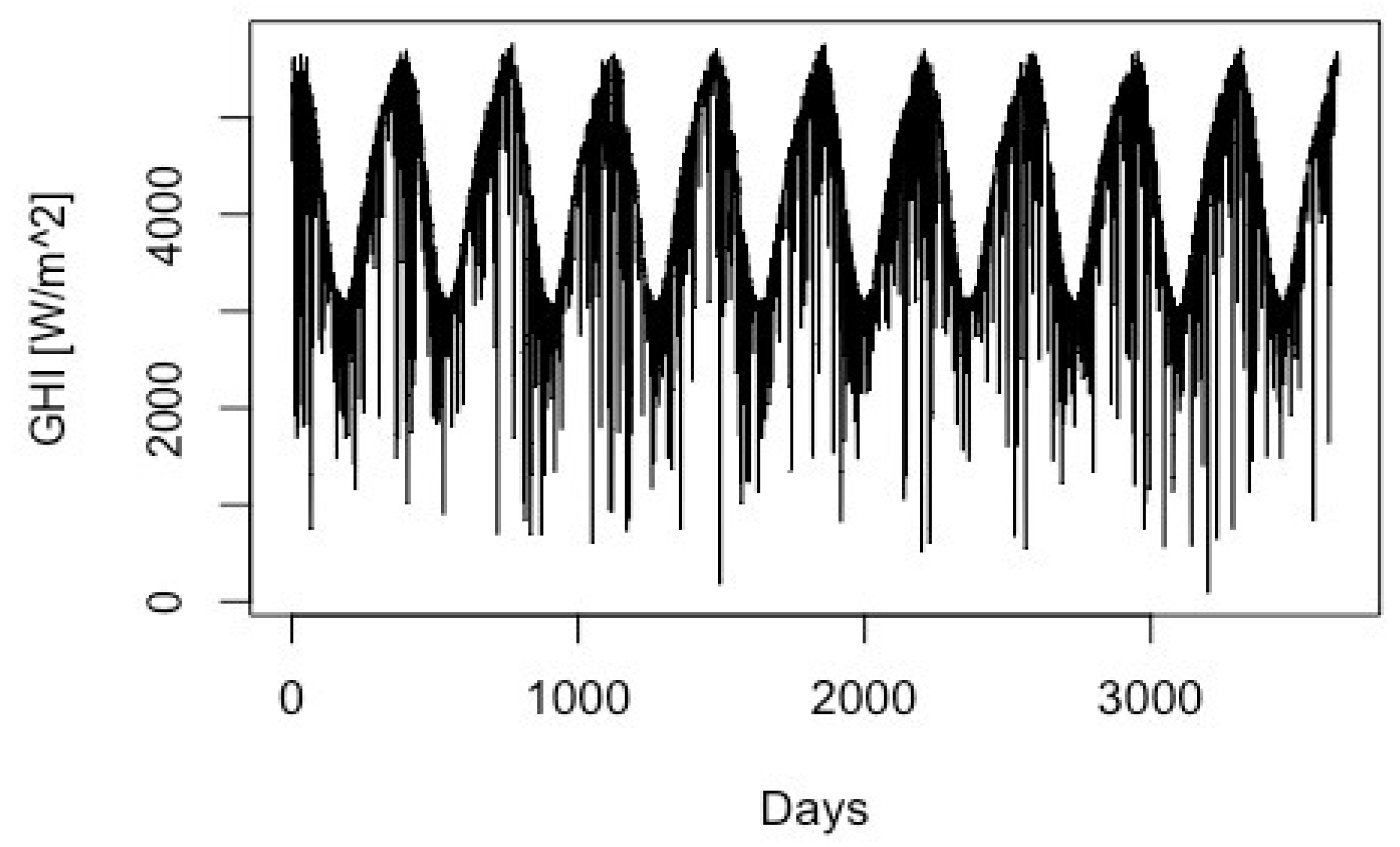
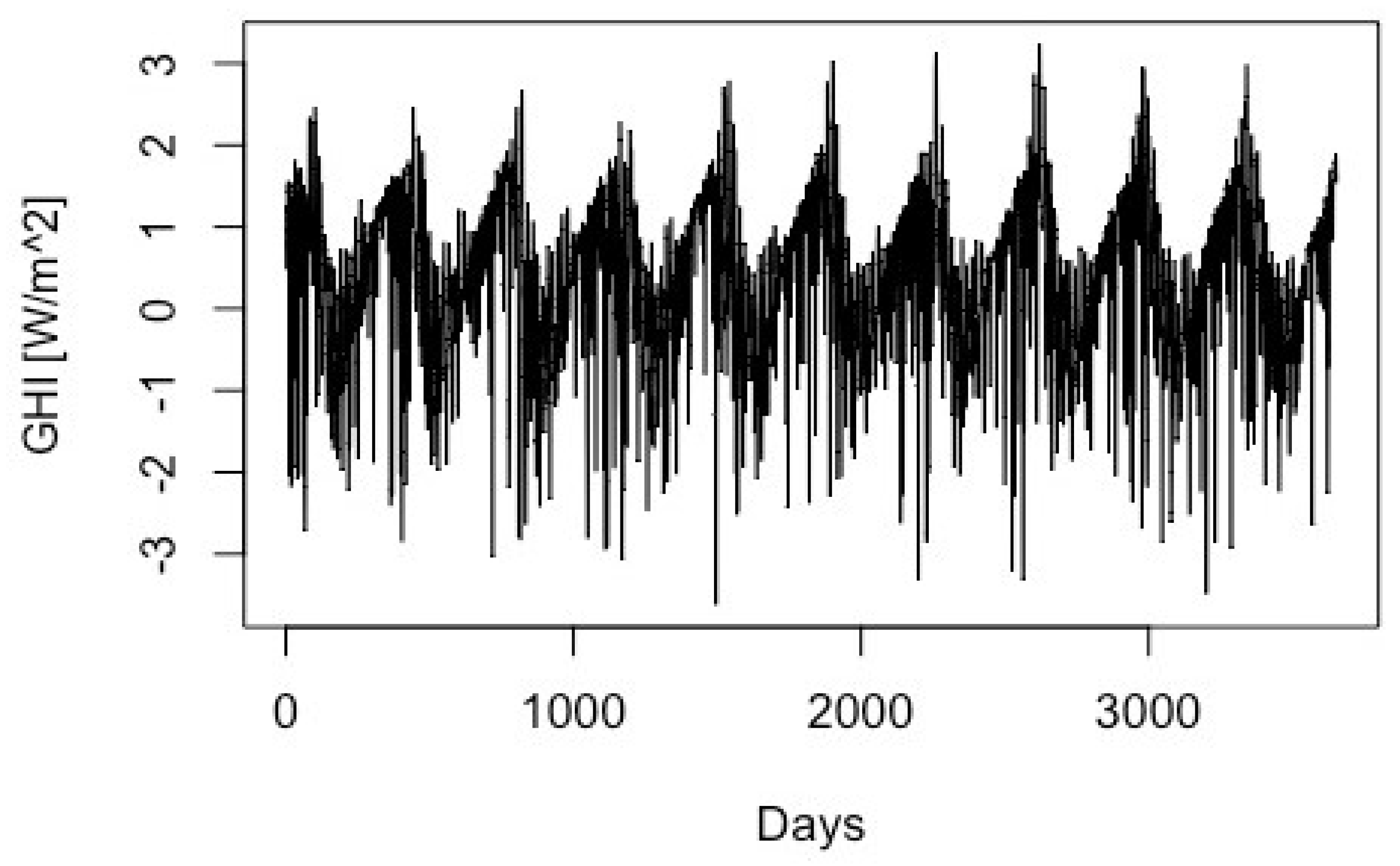
3.2. Daily Scale: Detrended and De-Seasonalized Data

The total amount of solar irradiation received at one place on the Earth’s surface and at a given latitude varies daily and seasonally. In order to overcome these two-time scale variabilities in each day, a filtering process was applied to the GHI dataset for de-trending and de-seasonalizing. The adjusted seasonal index method, which is a simple and convenient pre-processing method was used [25]. Let G(m,d) be GHI solar radiation observed at time m ( m [ 07 : 00 18 : 00 ] ) and day d ( d [ 1 / 1 / 2007 31 / 12 / 2016 ] ). The steps to compute the de-seasonalized GHI time series using the adjusted seasonal index method is as follows:
Step 1—Compute G ( d ) ¯   ,   which is the GHI daily mean:
G ( d ) ¯ = 1 M m = 1 M G ( m , d )
Step 2—Compute the modified GHI time series G m ( m , d ) by dividing the original time series G m , d   by its daily mean:
G m m , d = G ( m , d ) G ( d ) ¯
where G ( d ) ¯ is the GHI daily mean computed in step 1.
Step 3—Compute G ( m ) ¯ , which is the GHI climatological daily mean of the modified GHI time series G m ( m , d ):
G ( m ) ¯ = 1 D d = 1 D G m ( m , d )
Step 4—Compute AF, the adjusted factor of   G ( m ) ¯   :
A F = m = 1 M G ( m ) ¯ M
Step 5—Compute the deseasonalized adjusted GHI time series G d a ( m , d ) by dividing the modified GHI time series G m ( m , d ) (computed in Step 2) by the GHI climatologically daily mean G ( m ) ¯ (computed in Step 3), corrected by the adjusted factor AF (computed in Step 4):
G d a m , d = A F G m ( m , d ) ) G ( m ) ¯ .
The adjusted seasonal index method above has been used in this study; however, the results obtained present a low correlation coefficient (0.2~0.3) between 2 days. Based on this consideration, it is not practical to apply it to our satellite dataset (CM SAF). Thus, only normalization has been conducted for pre-processing.

3.3. Dataset Normalization

Normalization is the process of restructuring a relational database in accordance with a series of so-called normal forms in order to reduce data redundancy and improve data integrity. It was first proposed by [26]. If there is a dataset with various values or large differences between them, then it is better to obtain a more compact dataset through normalization. Normalization reduces dispersion of the collected data in order to obtain better results. Before performing the prediction, the training and test datasets were normalized. Figure 5 and Figure 6 show examples of the original and normalized GHI time series separately.

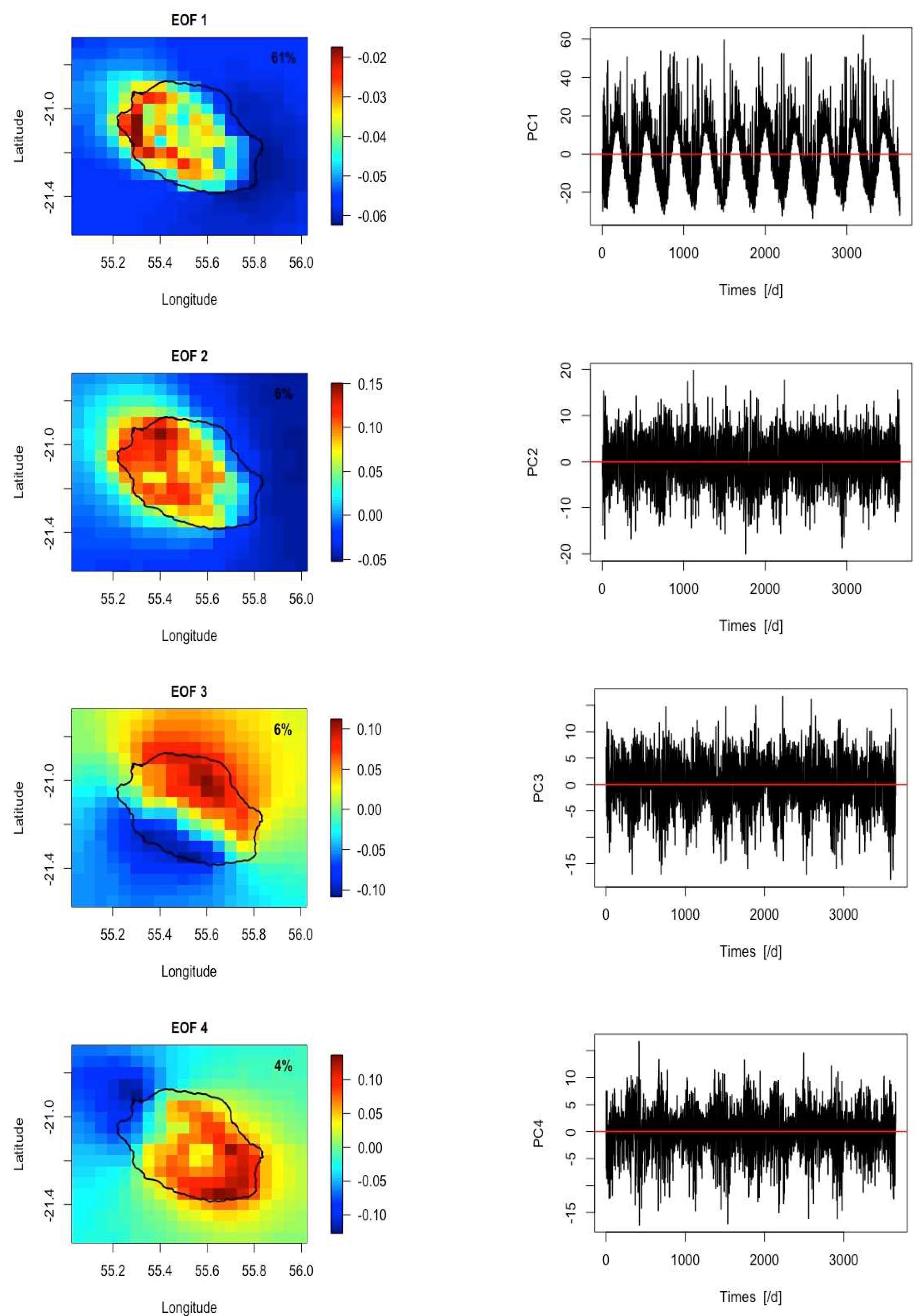
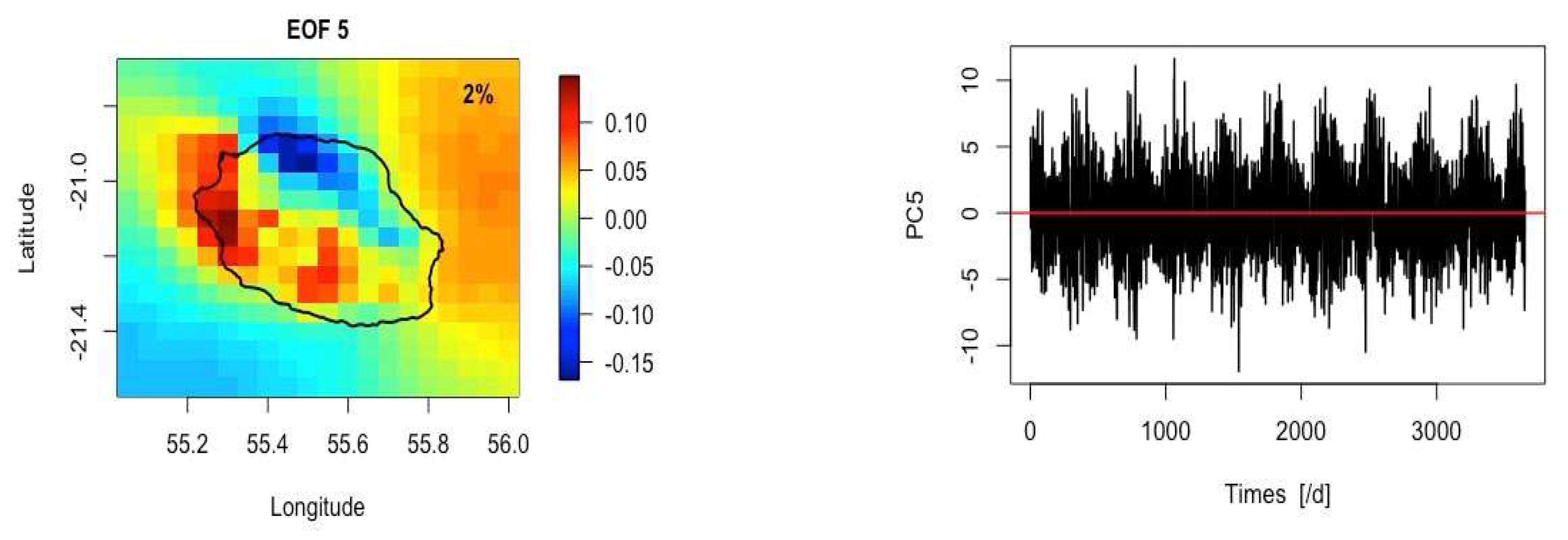
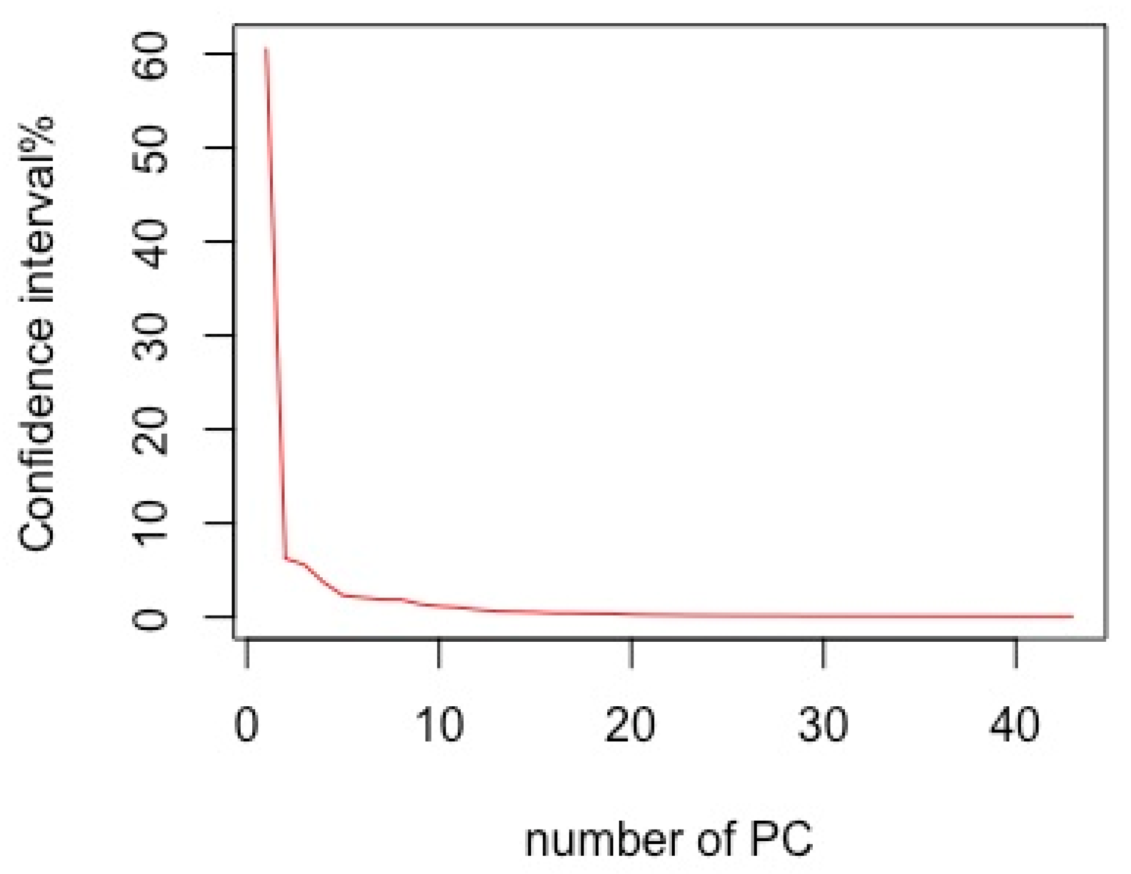
3.4. PCA Decomposition

There were four linear regression models used in this study, as mentioned above: SR, MLR, PCR, and PLSR. (1) SR: the first 3 days’ daily GHI in the domain area (all the grid points) are the independent variables in this linear model, and the dependent variable is the 4th day’s daily GHI in the domain area (all the grid points); (2) MLR: the independent variables are the first 3 days’ daily GHI at each grid point of the domain, and the dependent variable is the 4th day’s daily GHI at each grid point of the domain; (3) PCR: each PC obtained from the PCA analysis of GHI data is the independent variable, and the predicted PC is the dependent variable; (4) PLSR: each PC obtained from the PCA analysis of GHI data is the independent variable, and the predicted PC is the dependent variable.
PCA was applied to the GHI data in 2007~2016 in order to obtain the PCs. The PCs that could explain 95% of the variance were used as independent variables, and the predicted PCs are the dependent variables as output in the linear model. The first 5 PCs with their empirical orthogonal function (EOF) modes for the SSR data in 2007~2016 from CM SAF (SARAH-E@5km) are presented in Figure 7. EOF provided us with both the spatial and temporal patterns of the dominant modes of variability. The explained variance (%) of each PC is shown in Figure 8, and 43 PCs together can explain 95% of the variance. In Figure 7, it was observed that the leading 3 modes of EOF explained 61%, 6%, and 6% of the variance separately, and the first PC provides a greater contribution for SSR over Reunion Island. And these three PCs provide obviously different spatial distributions of SSR over Reunion Island: the first EOF mode showed more (less) SSR over the northwest (southwest) part; the second EOF mode showed more (less) SSR over the north (south) part; and the third EOF mode showed more (less) SSR over the northeast (southwest) part.

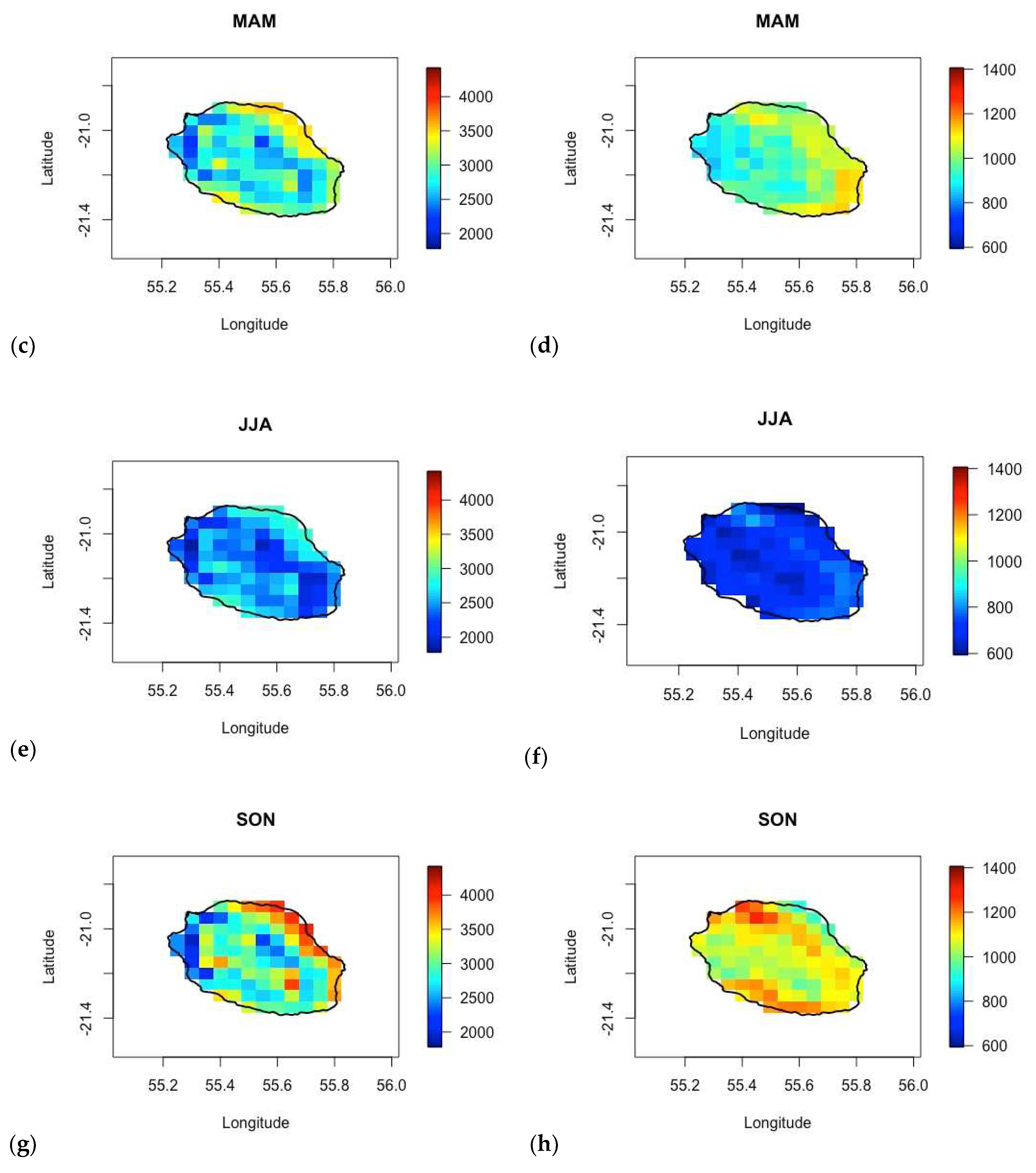
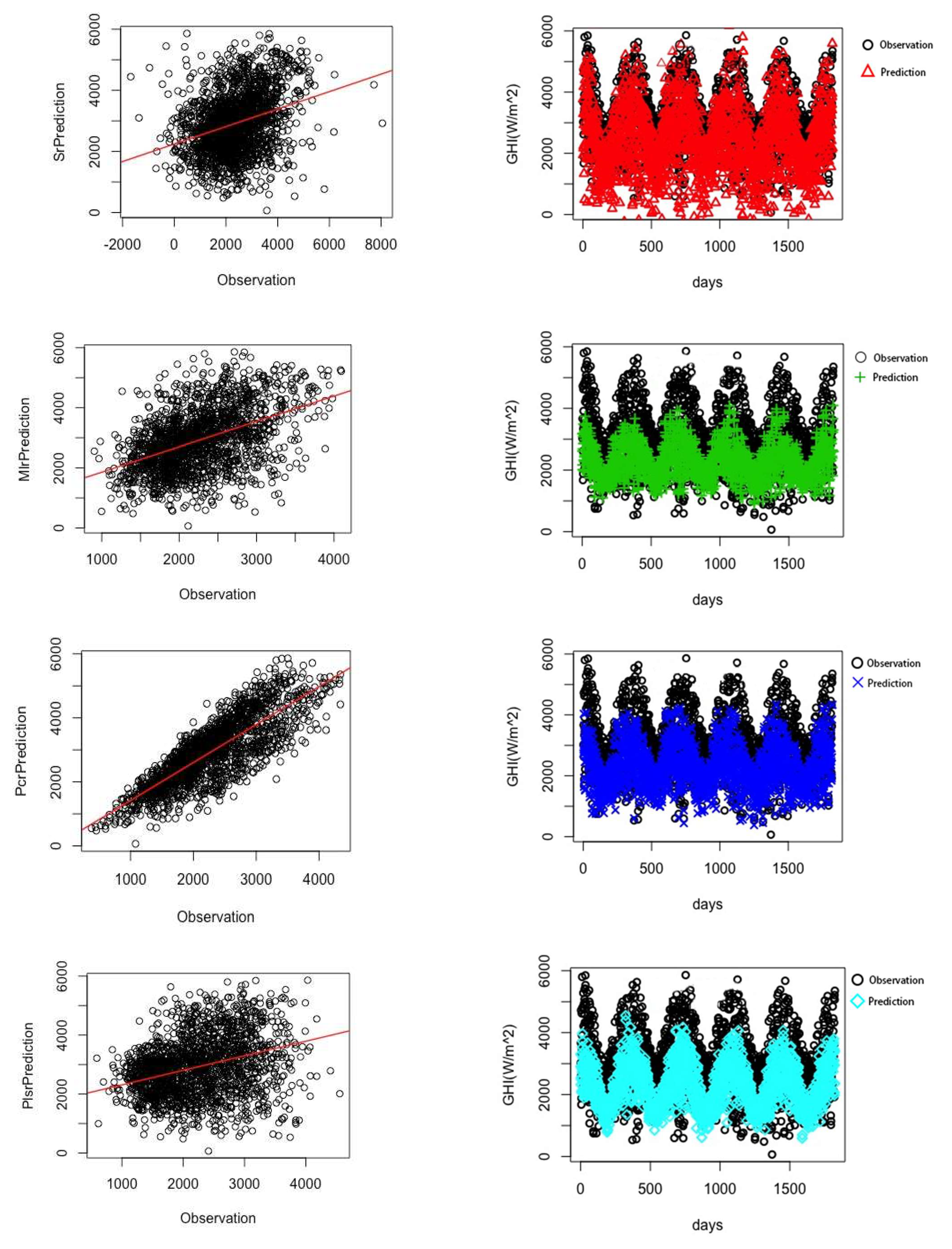
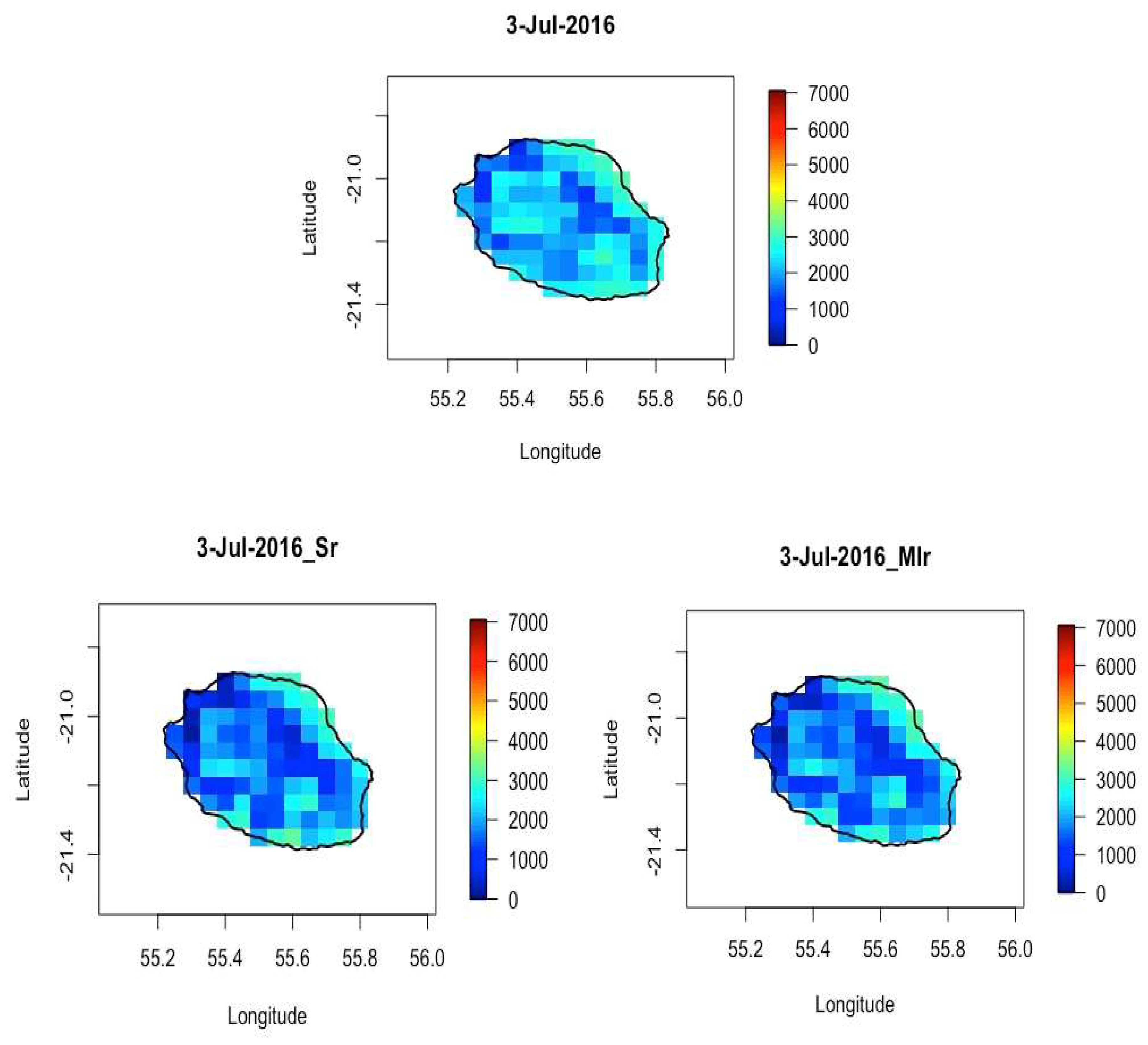
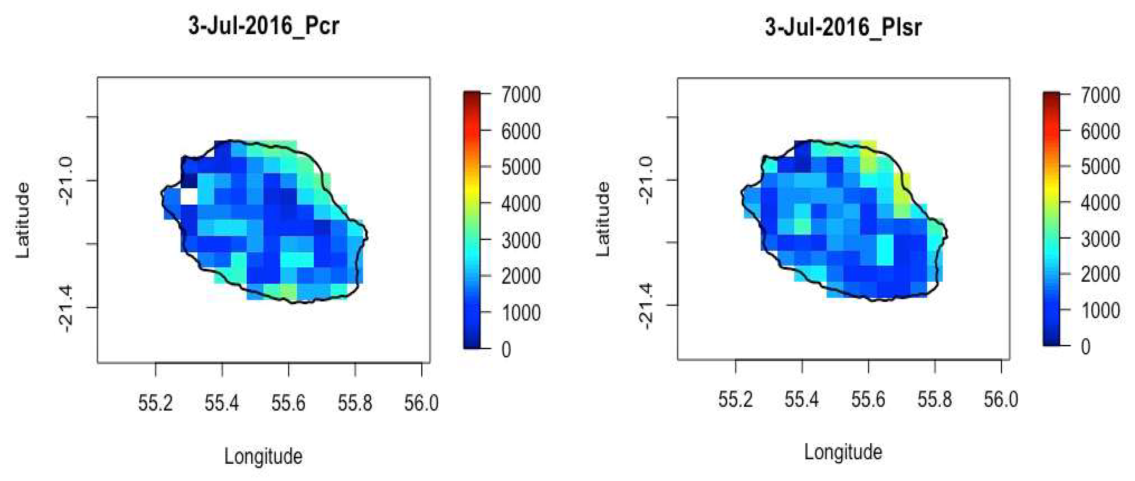
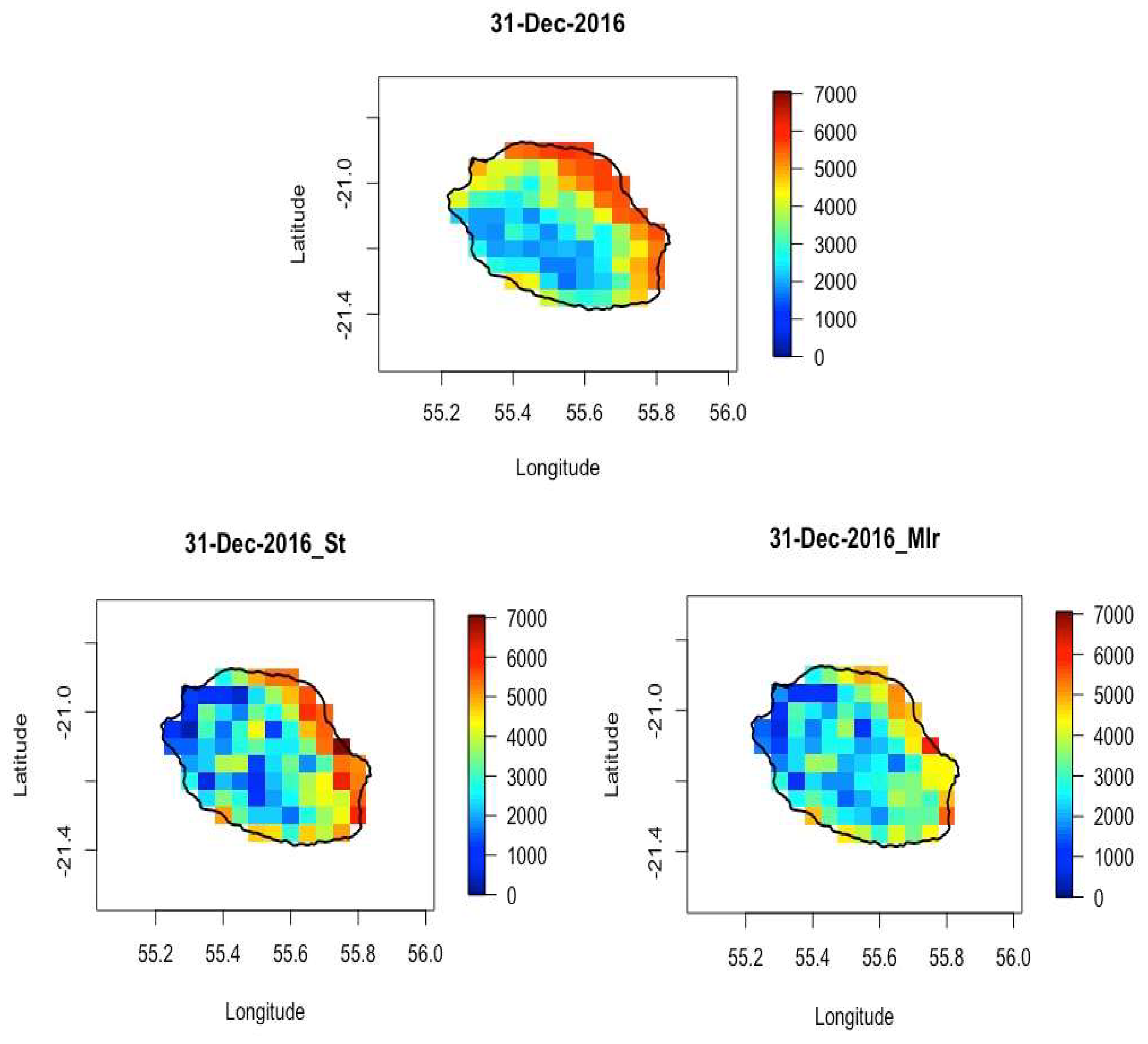
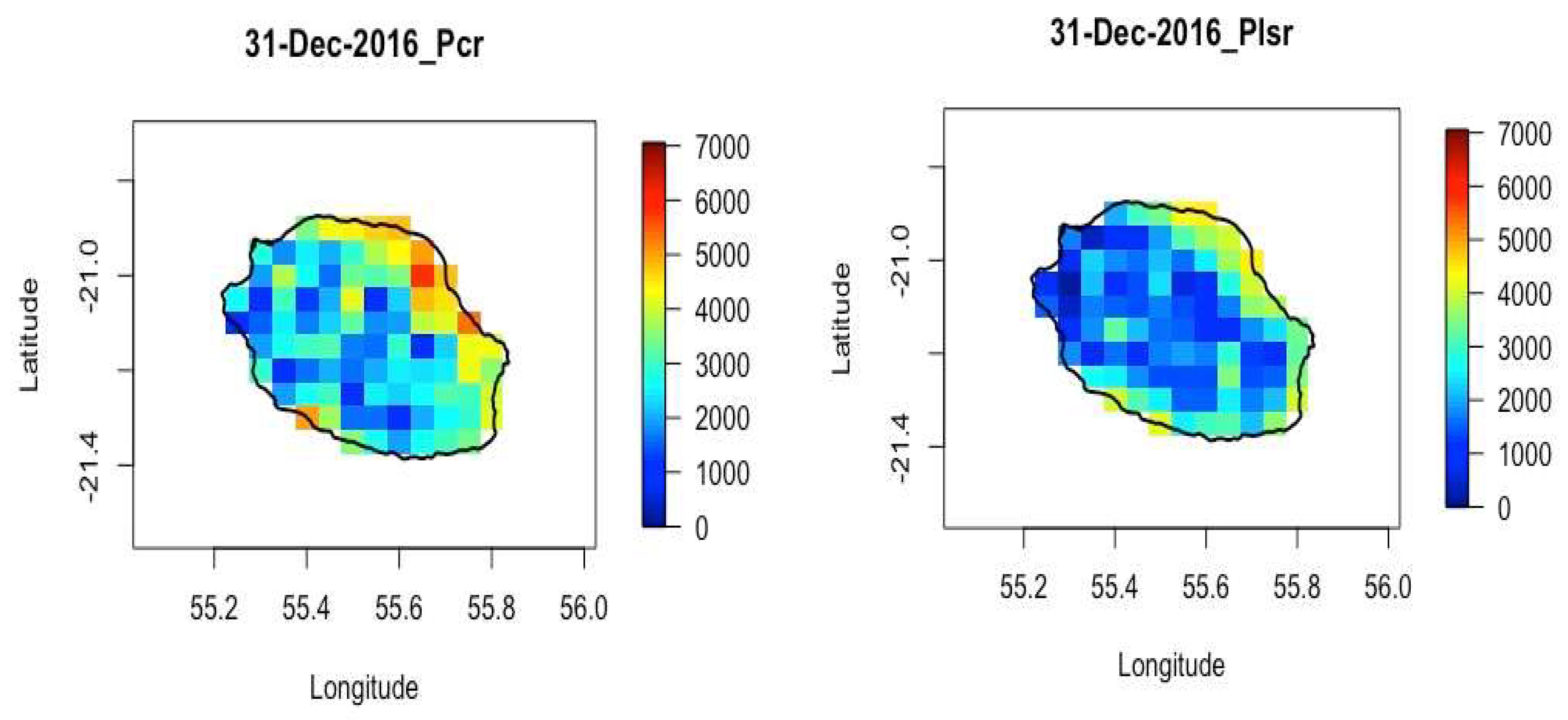
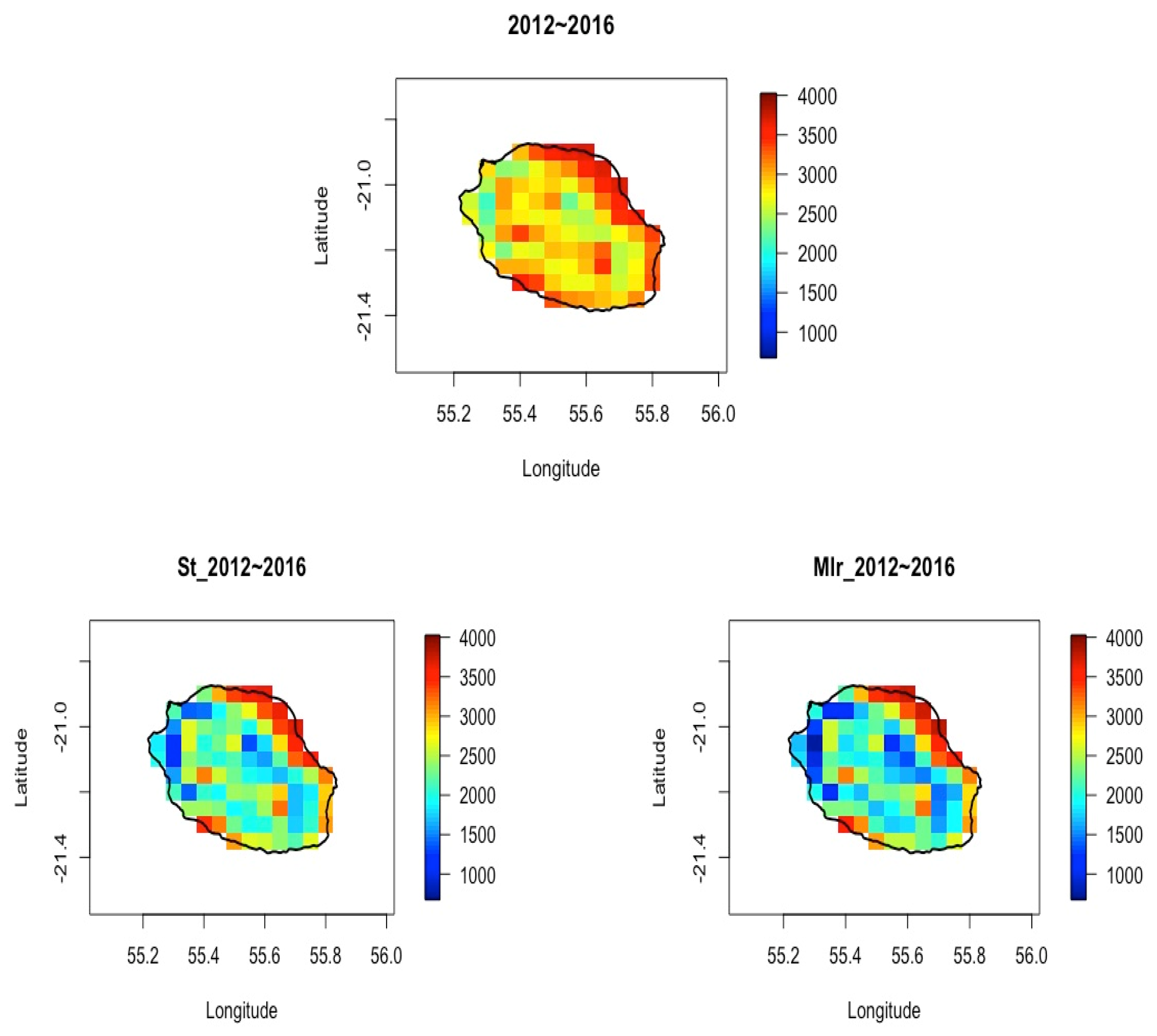
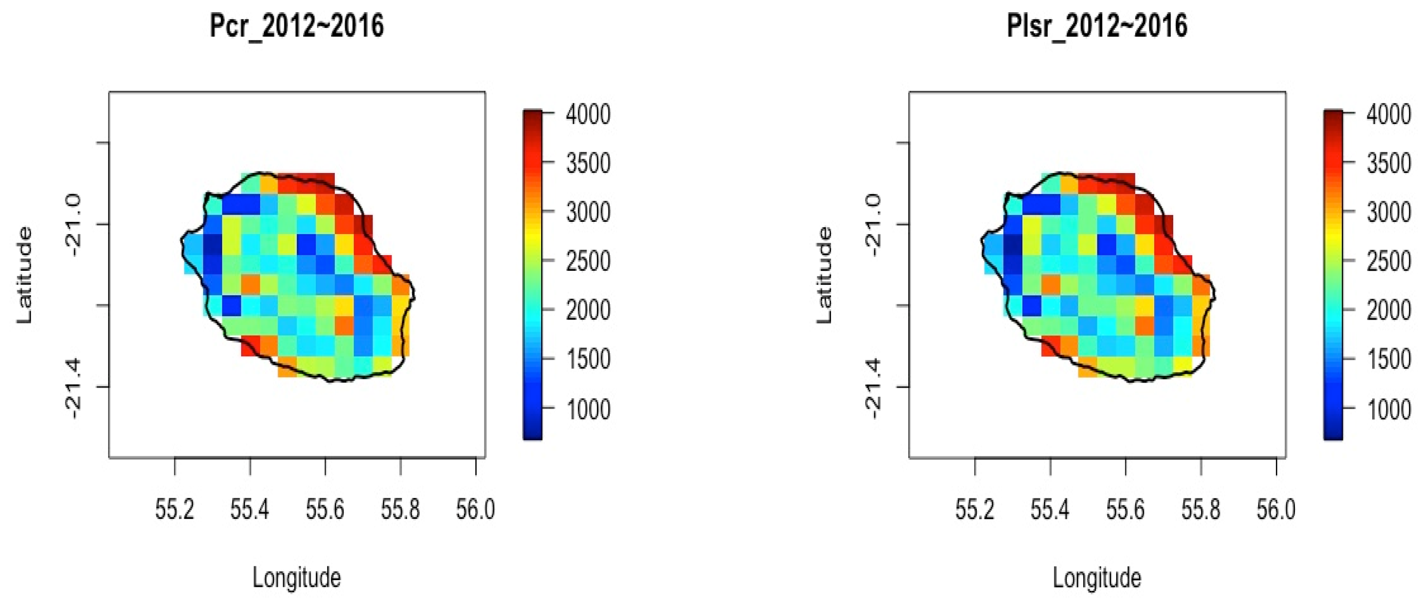
4. Prediction Results

4.1. Prediction Results with Four Linear Regression Models

Four linear regression models: SR, MLR, PCR, and PLSR were used in this study to predict SSR in 2007~2016 over Reunion Island. The 5 years of 2007–2011 were used as the training data and the 5 years of 2012~2016 as the test data. Figure 9 presents the goodness of fitting in a plot of prediction against observation (left panel) and comparing the daily prediction with observation (right panel) at one grid point over Reunion, for example, for the four linear regression models of 2012~2016. From this one grid point, the four models provide different predictions compared to the observations. For this one grid point, it can be seen at first that the PCR prediction model fits better with the observations. Even though the PCR predicted less SSR in the summer seasons than was observed, it provides a very accurate value in the winter seasons compared to SR (MLR/PLSR), which provides a relatively poor prediction for both summer and winter. Thus, PCR provides better prediction results than the other three models.
The re-mapping was conducted for the predicted data for spatial comparison over the whole island. The 3rd of July and the 31st of December 2016 were taken as two examples to show the mapping results (Figure 10 and Figure 11). These 2 days stand for the winter and summer seasons and could reflect the character of seasonal variability. The top mapping in Figure 10 and Figure 11 represents the observations, and the other four mappings in the bottom are the prediction mapping results from four linear regression models separately: SR, MLR, PCR, and PLSR.
In Figure 10, SR, MLR, PCR, and PLSR predictions all could present the obvious less SSR over the volcano area (Piton de la Fournaise) and the Cirque de Salazie compared to the observation on 3 July 2016. The four models show similar spatial variability of SSR over the other areas of the island, and it seems that the PCR model provides a closer SSR distribution (more SSR) over the southern coastal line as observed.
Figure 11 shows the observation of SSR on the 31st of December 2016 and the prediction due to the SR, MLR, PCR, and PLSR models, respectively. All four prediction models present more (less) daily SSR over the northeast (three cirques and the volcano) area compared to the observation.
Figure 12 shows the multi-annual mean of daily SSR mapping prediction with SR, MLR, PCR, and PLSR models in 2012~2016 compared to the observation. Four prediction models could all present more (less) daily SSR over the northeast (three cirques and the volcano) area as the observation in the next 5 years. PCR seems to provide less difference compared to the observations than the other models.

4.2. Score Evaluation: MAE, MSE, and RMSE

Based on the mapping prediction results with four linear regression models (SR, MLR, PCR, and PLSR), the statistical analysis using MAE, MSE, and RMSE was conducted. Table 1 lists the calculations for the four models. Table 1 shows that the PCR model had the smallest MAE, MSE, and RMSE compared to the other three models. The PCR model seems to be better for SSR mapping prediction over Reunion Island. Although the PCR model provides better prediction results, it can be seen that (MAE, MSE, and RMSE are quite large) the method was not quite accurate. Therefore, it is necessary to find a way to improve the accuracy of this prediction method.

5. Conclusions and Discussion

In this paper, a novel mapping prediction method for surface solar radiation with four linear regression models: MLR, PCR, SR, and PLSR, over Reunion Island, was used as a case study. Ten years of the SIS CM SAF SARAH-E dataset (0.05° × 0.05°), from 2007 to 2016, were first detrended, de-seasonalized, and normalized, then analyzed with PCA to obtain the input for the prediction models. Four linear regression models in the prediction were compared, which showed that SR, MLR, PCR, and PLSR predictions all presented obviously less SSR over the volcano area (Piton de la Fournaise) and the Cirque de Salazie compared to the observation. The four models showed similar spatial variability of SSR over the other areas of the island, and it seems that the PCR model provided closer SSR distribution (more SSR) over the southern coastal line, as observed.
All four prediction models presented more (less) daily SSR over the northeast (three cirques and the volcano) area compared to the observation. The multi-annual mean of the daily SSR mapping prediction with SR, MLR, PCR, and PLSR models for 2012~2016 compared to the observation shows that the four prediction models could all present more (less) daily SSR over the northeast (three cirques and the volcano) area than the observation during 2012~2016. PCR seems to provide less difference compared to the observations than the other models. The statistical analysis using MAE, MSE, and RMSE shows that the PCR model had the smallest MAE, MSE, and RMSE compared to the other three models. The PCR model seems better for SSR mapping prediction over Reunion Island. Although the PCR model provided better prediction results, its MAE, MSE, and RMSE were quite large. Therefore, it is necessary to find a way to improve the accuracy of this prediction method in the future. At the same time, this study was an exploration to test linear regression models’ capability for SSR mapping prediction. For Reunion Island’s complex terrain, geographical location, and abundant energy resources, and to solve the limitations of this study a novel method will be used in future work.

Author Contributions

Conceptualization, M.B. and Q.L.; Methodology, M.B. and Q.L.; Software, Q.L. and P.L.; Validation, Q.L. and P.L.; Formal analysis, Q.L.; Investigation, Q.L. and P.L.; Writing—original draft preparation, Q.L. and P.L.; Writing—review and editing, Q.L. and P.L.; Visualization, Q.L. and P.L.; Supervision, M.B.; Project administration, M.B.; Funding acquisition, M.B. All authors have read and agreed to the published version of the manuscript.

Funding

This study was financed by the Europe and Region Reunion (Tiers:181727-Dossier N.: D2013032473).

Institutional Review Board Statement

Not applicable.

Informed Consent Statement

Not applicable.

Data Availability Statement

Study data can be obtained from the EUMETSAT Satellite Application Facility on Climate Monitoring (CM SAF) via website.

Acknowledgments

The authors would like to thank lab LE2P at the University of Reunion for providing the surface solar radiation dataset. The authors also thank the EUMETSAT Satellite Application Facility on Climate Monitoring (CM SAF) for providing the available validation dataset. This work was supported by the Europe and Region Reunion (Tiers:181727-Dossier N.: D2013032473). The authors thank the anonymous reviewers for their useful comments and suggestions.

Conflicts of Interest

The authors declare no conflict of interest.

References

  1. Jean, P.P.; Mathieu, D.; Frantz, S.; Dominique, M.; Olivier, M. Renewable energy: Progressing towards a net zero energy island, the case of Reunion Island. Renew. Sustain. Energy Rev. 2012, 16, 426–442. [Google Scholar]
  2. Chrystel, D.; Vincent, F.; Bruno, T.; Jean-Michel, B.; Bhavani, B. Potential areas of interest for the development of geothermal energy in La Reunion Island based on GIS analysis. J. Volcanol. Geotherm. Res. 2022, 421, 107450.1–107450.13. [Google Scholar]
  3. Dosseto, A.; Hannan-Joyner, A.; Raines, E.; Gayer, E.; Michon, L. Geochemical evolution of soils on Reunion Island. Geochim. Cosmochim. Acta 2022, 318, 263–278. [Google Scholar] [CrossRef]
  4. Gueymard, C.A. Direct solar transmittance and irradiance prediction with broadband models. Part I: Detailed theoretical performance assessment. Sol. Energy 2003, 74, 355–379. [Google Scholar] [CrossRef]
  5. Boata, R.; Pop, N. Estimation of global solar irradiation by using takagi-sugeno fuzzy systems. Rom. J. Phys. 2015, 60, 593–602. [Google Scholar]
  6. Calinoiu, D.; Stefu, N.; Boata, R.; Blaga, R.; Pop, N.; Paulescu, E.; Sabadus, A.; Paulescu, M. Parametric modeling: A simple and versatile route to solar irradiance. Energy Convers. Manag. 2018, 164, 175–187. [Google Scholar] [CrossRef]
  7. Chevillon, L.; Tourmetz, J.; Dubos, J.; Soulaimana-Mattoir, Y.; Hollinger, C.; Pinet, P.; Couzi, F.X.; Riethmuller, M.; Le Corre, M. 25 years of light-induced petrel groundings in Reunion Island: Retrospective analysis and predicted trends. Glob. Ecol. Conserv. 2022, 33, e02232. [Google Scholar] [CrossRef]
  8. Oyewola, O.M.; Patchali, T.E.; Ajide, O.O.; Singh, S.; Matthew, O.J. Global solar radiation predictions in Fiji Islands based on empirical models. Alex. Eng. J. 2022, 61, 8555–8571. [Google Scholar] [CrossRef]
  9. Bamisile, O.; Oluwasanmi, A.; Ejiyi, C.; Yimen, N.; Obiora, S.; Huang, Q. Comparison of machine learning and deep learning algorithms for hourly global/diffuse solar radiation predictions. Int. J. Energy Res. 2021, 46, 10052–10073. [Google Scholar] [CrossRef]
  10. Zhang, C.; Hua, L.; Ji, C.; Nazir, M.S.; Peng, T. An evolutionary robust solar radiation prediction model based on WT-CEEMDAN and IASO-optimized outlier robust extreme learning machine. Appl. Energy 2022, 322, 119518. [Google Scholar] [CrossRef]
  11. Ghimire, S.; Nguyen-Huy, T.; Deo, R.C.; Casillas-Perez, D.; Salcedo-Sanz, S. Efficient daily solar radiation prediction with deep learning 4-phase convolutional neural network, dual stage stacked regression and support vector machine CNN-REGST hybrid model. Sustain. Mater. Technol. 2022, 32, e00429. [Google Scholar] [CrossRef]
  12. Pang, Z.; Niu, F.; O’Neill, Z. Solar radiation prediction using recurrent neural network and artificial neural network: A case study with comparisons. Renew. Energy 2020, 156, 279–289. [Google Scholar] [CrossRef]
  13. Nwokolo, S.C.; Obiwulu, A.U.; Ogbulezie, J.C.; Amadi, S.O. Hybridization of statistical machine learning and numerical models for improving beam, diffuse and global solar radiation prediction. Clean. Eng. Technol. 2022, 9, 100529. [Google Scholar] [CrossRef]
  14. Diagne, M.H.; David, M.; Boland, J.; Schmutz, N.; Lauret, P. Post-processing of Solar Irradiance Forecasts from WRF Model at Reunion Island. In Energy Procedia; Elsevier: Amsterdam, The Netherlands, 2014; Volume 57, pp. 1364–1373. [Google Scholar]
  15. Lauret, P.; Voyant, C.; Soubdhan, T.; David, M.; Poggi, P. A benchmarking of machine learning techniques for solar radiation forecasting in an insular context. Sol. Energy 2015, 112, 446–457. [Google Scholar] [CrossRef]
  16. Li, P.; Bessafi, M.; Morel, B.; Chabriat, J.P.; Delsaut, M.; Li, Q. Daily surface solar radiation prediction mapping using artificial neural network: The case study of Reunion Island. J. Sol. Energy Eng. 2019, 142, 21009-1–21009-8. [Google Scholar] [CrossRef]
  17. Li, P.; Morel, B.; Bessafi, M.; Li, Q.; Chiacchio, M. Radiation budget in RegCM4: Simulation results from two radiative schemes over the South West Indian Ocean. Clim. Res. 2021, 48, 181–195. [Google Scholar] [CrossRef]
  18. Huld, T.; Müller, R.; Gracia-Amillo, A.; Pfeifroth, U.; Trentmann, J. Surface Solar Radiation Data Set—Heliosat, Meteosat-East (SARAH-E)—Edition 1.1; Satellite Application Facility on Climate Monitoring: Offenbach, Germany, 2017. [Google Scholar] [CrossRef]
  19. Gracia Amillo, A.; Huld, T.; Müller, R. A new database of global and direct solar radiation using the Eastern Meteosat Satellite, models and validation. Remote Sens. 2014, 6, 8165–8189. [Google Scholar] [CrossRef]
  20. Altman, N.S. An introduction to kernel and nearest-neighbor nonparametric regression. Am. Stat. 1992, 46, 175–185. [Google Scholar]
  21. Kutzbach, J.E. Empirical Eigenvectors of Sea-Level Pressure, Surface Temperature and Precipitation Complexes over North America. J. Appl. Meteorol. 1967, 6, 791–802. [Google Scholar] [CrossRef]
  22. Wilks, P.A.D.; English, M.J. A system for rapid identification of respiratory abnormalities using a neural network. Med. Eng. Phys. 1995, 17, 551–555. [Google Scholar] [CrossRef] [PubMed]
  23. Jolliffe, I.T. Principal Component Analysis, 2nd ed.; Springer: Berlin/Heidelberg, Germany, 2002. [Google Scholar]
  24. Badosa, J.; Haeffelin, M.; Chepfer, H. Scales of spatial and temporal variation of solar irradiance on Reunion tropical island. Sol. Energy 2013, 88, 42–56. [Google Scholar] [CrossRef]
  25. Brockwell, P.J.; Davis, R.A. Time Series: Theory and Methods; Springer Series in Statistics; Springer: Berlin/Heidelberg, Germany, 1986. [Google Scholar]
  26. Codd, E.F. A Relational Model of Data for Large Shared Data Banks. Commun. ACM 1970, 13, 377–387. [Google Scholar] [CrossRef]
Figure 1. Annual average of global horizontal irradiance (kWh/m2) distribution [1].
Atmosphere 14 01331 g001
Figure 2. Flowchart of the prediction process and methods.
Atmosphere 14 01331 g002
Figure 3. The seasonal mean and standard deviation of SSR in summer, winter, and inter-season from 2007 to 2016 (10 years) over Reunion Island.
Atmosphere 14 01331 g003
Figure 4. The seasonal mean (a,c,e,g) and standard deviation (b,d,f,h) of SSR in the summer, winter, and inter-season from 2007 to 2016 over Reunion (W/m2).
Atmosphere 14 01331 g004aAtmosphere 14 01331 g004b
Figure 5. The original GHI time series with the trend for the years 2007~2016.
Atmosphere 14 01331 g005
Figure 6. The normalized daily time series 2007~2016 in one grid point of Reunion.
Atmosphere 14 01331 g006
Figure 7. The leading five EOF modes (left panel) for GHI for its PCs (right panel) in 2007~2016.
Atmosphere 14 01331 g007aAtmosphere 14 01331 g007b
Figure 8. The explained variance (%) of each PC.
Atmosphere 14 01331 g008
Figure 9. The goodness of fitting in a plot of prediction against observation (left panel) and comparing the daily prediction with observation (right panel) at one grid point in 2012~2016 over Reunion (W/m2).
Atmosphere 14 01331 g009
Figure 10. The SSR prediction mapping with four different linear regression methods against the original mapping (W/m2) on 3 July 2016.
Atmosphere 14 01331 g010aAtmosphere 14 01331 g010b
Figure 11. The SSR prediction mapping with four different linear regression methods against the original mapping (W/m2) on 31 December 2016.
Atmosphere 14 01331 g011aAtmosphere 14 01331 g011b
Figure 12. The multi-annual mean of daily SSR mapping prediction with SR, MLR, PCR, and PLSR models in 2012~2016 compared to the observations.
Atmosphere 14 01331 g012aAtmosphere 14 01331 g012b
Table 1. Statistics of linear regression models.
MAE (W/m2)MSERMSE (W/m2)
SR1.142 × 1032.15× 1061.47 × 103
MLR1.00 × 1031.58× 1061.26 × 103
PCR7.97 × 1029.24× 1059.61 × 102
PLSR1.11 × 1031.93× 1061.39 × 103
Disclaimer/Publisher’s Note: The statements, opinions and data contained in all publications are solely those of the individual author(s) and contributor(s) and not of MDPI and/or the editor(s). MDPI and/or the editor(s) disclaim responsibility for any injury to people or property resulting from any ideas, methods, instructions or products referred to in the content.

