Integrating Ensemble Weather Predictions in a Hydrologic-Hydraulic Modelling System for Fine-Resolution Flood Forecasting: The Case of Skala Bridge at Evrotas River, Greece

Abstract

Ensemble weather forecasting involves the integration of multiple simulations to improve the accuracy of predictions by introducing a probabilistic approach. It is difficult to accurately predict heavy rainfall events that cause flash floods and, thus, ensemble forecasting could be useful to reduce uncertainty in the forecast, thus improving emergency response. In this framework, this study presents the efforts to develop and assess a flash flood forecasting system that combines meteorological, hydrological, and hydraulic modeling, adopting an ensemble approach. The integration of ensemble weather forecasting and, subsequently, ensemble hydrological-hydraulic modeling can improve the accuracy of flash flood predictions, providing useful probabilistic information. The flash flood that occurred on 26 January 2023 in the Evrotas river basin (Greece) is used as a case study. The meteorological model, using 33 different initial and boundary condition datasets, simulated heavy rainfall, the hydrological model, using weather inputs, simulated discharge, and the hydraulic model, using discharge data, estimated water level at a bridge. The results show that the ensemble modeling system results in timely forecasts, while also providing valuable flooding probability information for 1 to 5 days prior, thus facilitating bridge flood warning. The continued refinement of such ensemble multi-model systems will further enhance the effectiveness of flash flood predictions and ultimately save lives and property.

1. Introduction

The continuous interaction of physical processes between the atmosphere and hydrosphere has a profound impact on the planet’s water cycle. This interplay, at times, can give rise to severe hydrometeorological phenomena, such as floods [1]. Flooding stands out as one of the most recurrent natural hazards, consistently endangering human lives and essential infrastructure. Over the past three decades, floods exhibit an overall increasing trend worldwide [2], underscoring the necessity to increase preparedness and the timely and efficient protection of socio-economic activities and human lives [3,4]. It is difficult to be sure that flood protection measures or defense structures can be completely effective, especially under changing climate conditions [1]. Thus, it becomes crucial for flood-risk management systems to be able to provide timely forecasts, warnings, and ample lead time, which is necessary both for human safety and for the timely application of interventions [5,6,7,8]. Therefore, it is very important to build robust flood forecasting systems, considering real weather conditions, providing thus scientifically supported inputs for informed decision making, enhancing the resilience to floods [9,10].

The need to enable the anticipation of impending heavy rainfall events and their potential impact on hydrological systems leading to potential flooding has long been recognized and researched [11]. The inherent uncertainties concerning meteorological phenomena that pass through flood models and forecasts have also long been researched [12,13], and continue to be a crucial research question [14], given the importance of accurate and timely forecasts [15], and the need for considering climate and weather uncertainties in integrated planning [16]. In that context, probabilistic forecasts have been proved particularly useful in enhancing the reliability of hydrologic-hydraulic forecasts [17]. Ensembles have found several applications in weather forecasting [18], given their ability to use multiple simulations based on slight variations in initial conditions and/or parameters, capturing a range of potential outcomes and associated uncertainties in predicting meteorological processes, even with limited data [19,20,21]. Unlike traditional deterministic approaches that offer a single prediction, ensembles offer a spectrum of outcomes, capturing complexities and uncertainties. This is crucial for a more realistic and comprehensive understanding of hydrometeorological-hydraulic systems, enhancing risk management and response planning, compared to relying on a single-point deterministic prediction, which can often be misleading [22].

Previous papers using ensemble forecasting alert systems for flood forecasts usually provide short-term predictions, and they refer to large scale study areas. For example, the Iowa Flood Center (IFC) has operated a flood forecasting and information dissemination system across the state since 2008, which is based on 15-min forecasts [23]. Other ensemble forecasting alert systems developed for the Cévennes–Vivarais region (Southern France) have been able to provide forecasts even 48 hours ahead of a flood event, for medium-sized catchments covering 100–600 km² [24]. Similar flood warning applications based on ensemble forecasts have been developed for Iranian catchments of similar size (Kan Basin, approximately 200 km²) [25]. There are large scale applications (large scale hydrology), such as the European Flood Awareness System (EFAS) based on medium-range weather forecasts [5], considering large basins, such as the Danube river basin [26]. Ming et al. [27] have developed a flood forecasting system for the 2500 km² Eden Catchment, England, with a lead time of 34 h. However, the above examples are based on two models, at most, to cope with the large scale computational demand, and also manage to provide results of adequate lead time. In particular, these applications are usually based on a weather forecast model, the results of which are then used to estimate the flood peaks by other methods (including Bayesian Networks, MultiCriteria Analysis, Machine Learning), considering only the rainfall peak thresholds [28,29], or use Machine Learning to capture modelling uncertainties directly for flood simulations [30], while rarely employing hydraulic models [18]. There are significantly fewer applications capturing the meteorological conditions and uncertainties through weather forecast models and exploring their progression through comprehensive hydrological and hydraulic models. Moreover, the level of detail of the existing applications, in relation to their lead time, is a challenge [28], as it is difficult to provide accurate forecasts at small catchment scales and with sufficient lead time exceeding 24–48 h [22]. Thus, there are fewer small-scale applications of fine resolution, where the accuracy and modelling detail are difficult to be adequately captured. The review article by Todini [22] highlights the need for enhanced probabilistic forecasts, based on EFAS, and calls for improved and more integrated modelling approaches, able to provide adequate lead time forecasts for fine scales. The review on ensemble-based flood forecasting applications by Wu et al. [18] is in line with the above, and further highlights the need to thoroughly assess uncertainties from multiple sources and models.

In this paper, we aim to fill these gaps by: (a) using an integrated system combining three models (meteorologic, hydrologic, hydraulic); (b) analyzing a real flash-flood event in high-resolution at a small scale (a bridge in a Greek catchment); (c) aiming to provide the initial flood alert signals five days prior to the flood event. In particular, we combined the Advanced Weather Research and Forecasting (WRF–ARW) model, which was ‘fed’ with ensemble probabilistic forecasts, the WRF–Hydro hydrological model, and the HEC–RAS hydraulic–hydrodynamic model. This allows us to assess the uncertainties in each modelling stage (weather, streamflow, water depth). The small scale is a comparative advantage over existing approaches, including the sole other application of this system [31] (which, however, did not consider an ensemble forecasting and, thus, an uncertainty assessment). In this work, the small-scale precision was achieved by exploiting analyses from Remote Sensing for our study area, along with data obtained from drones, to create a refined terrain model, allowing us to focus even on specific infrastructure elements (i.e., a small bridge) to showcase its flooding probability under a real-world event. To our knowledge, this is the first application (at least in Greece), of such a holistic modelling approach at a scale that other ensemble forecasting alert systems currently cannot assess in such detail. Our ensemble approach considered a forecast up to five days prior to the flood event, which also allowed us to assess the behaviour of uncertainty as the event progressed, and the ability to provide robust alerts. The novelty of the presented approach lies in its integrated character, combining and advancing multiple models and methods, its fine resolution at all modelling stages, the ambitious early warning signals, and its operational character that enables its application to other areas.

2. Study Area, Models and Methods

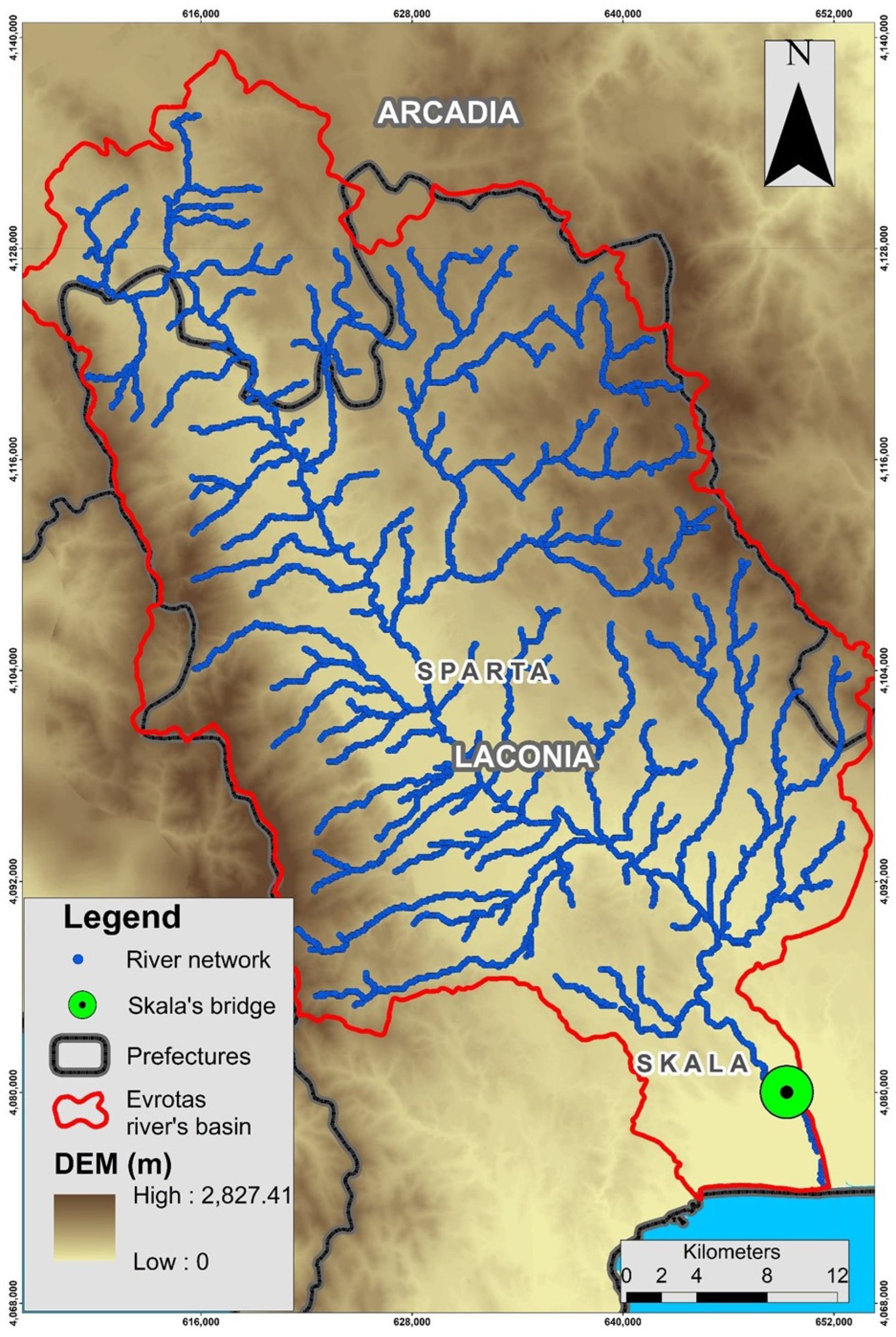
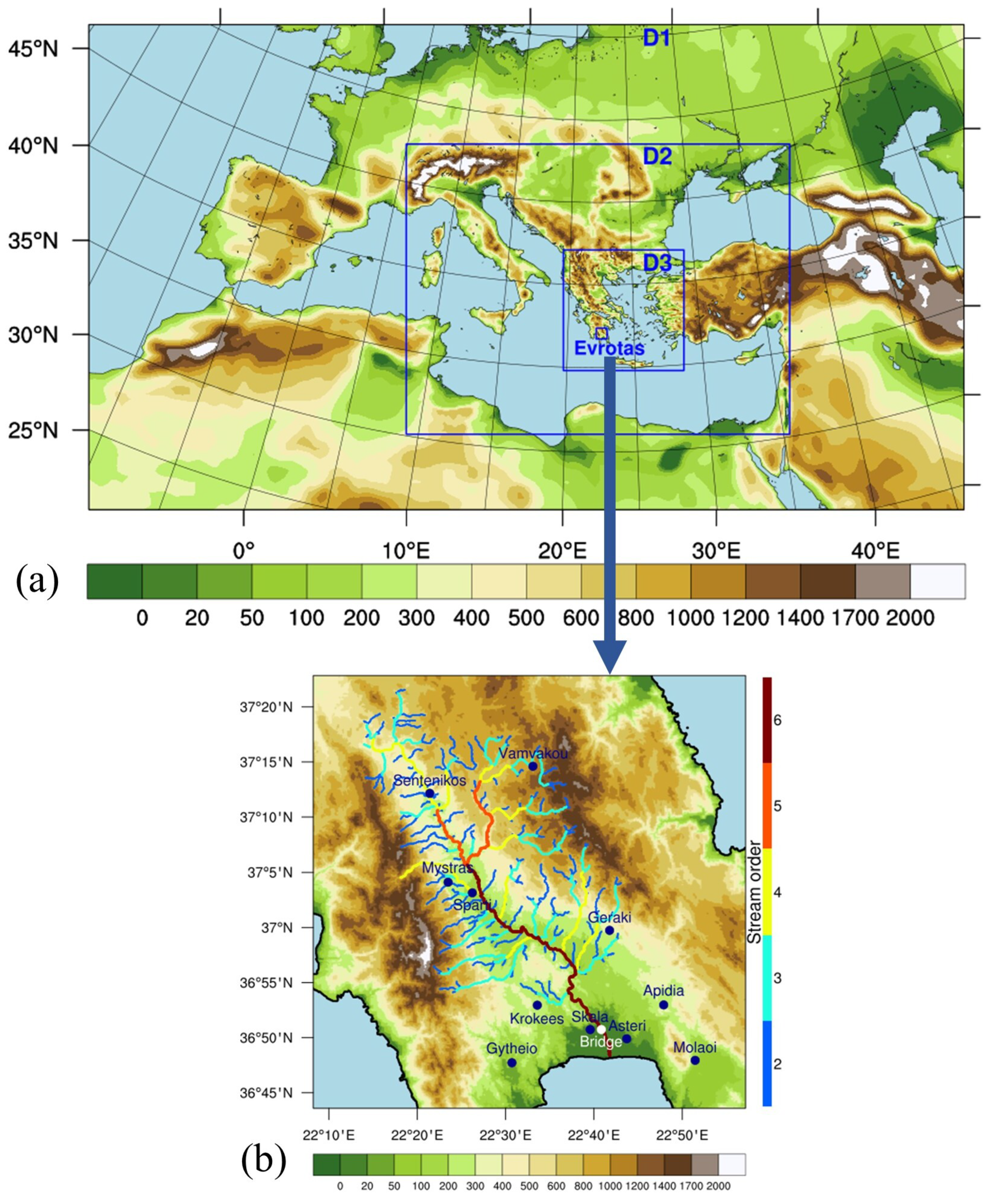
2.1. Study Area

Evrotas is one of the largest rivers at the southern end of the Balkan Peninsula [32]. Its basin is located in the south-eastern part of Peloponnese (Greece), covering approximately 2400 km². Evrotas River Basin (ERB) originates from the regional unit of Arcadia, while most of the river crosses the regional unit of Laconia and flows in a northwest–southeast direction for approximately 90 km before discharging into the Laconic Gulf [33] (Figure 1).

Almost 41% of the ERB has elevations that are higher than 600 m.a.s.l. (meters above sea level) and 46% of the area is characterized by elevations ranging from 150 to 600 m.a.s.l. The southwestern part of the basin presents the steepest slopes (45%), while the average slope is 20%. Concerning the observed land uses, most of the basin (70%) is covered by low vegetated areas, native coniferous and mixed forests, while the rest of the area accommodates mostly agricultural activities. Regarding the geological formations, 42% of the catchment is covered by carbonate formations while, mostly along the plain areas, riverine sediments of Neogene or more recent age are detected [34]. The ERB is defined by a Mediterranean climate type with hot, dry summers and cool, wet winters, with mean annual precipitation and air temperature of 800 mm and 16 °C, respectively.

In general, the ERB is characterized by a hydrological complexity as it presents perennial, intermittent, ephemeral and episodic river flows combined, in some places, with interactive groundwater [34]. In summer or extended dry periods, the hydraulic connectivity of the river is interrupted in certain areas. This interruption occurs because water flows downward into carbonate karstic formations and due to excessive extraction from nearby aquifers for irrigation purposes [34]. On the other hand, river parts that preserve the flow are mainly dependent on karstic springs located along the river [35]. The river flow is regenerated after the Skala region, located in the agricultural plain of the Evrotas River Delta (Figure 1), due to its recharge with groundwater through springs [33].

Furthermore, during the winter period, large flash flood events occur with disastrous impacts on infrastructure, agricultural areas, and human lives [34,36]. For example, the flash flood that occurred on 7 September 2016 caused one fatality, severe damage, and the overflow of the bridge of the town of Skala [37] (Figure 1). This paper focuses on a more recent flash flood event, that occurred on 26 January 2023. This flood resulted in damage to roads, cultivation and buildings, among other infrastructure elements and properties (Figure 2). It inflicted severe damage, particularly in agricultural areas, as the majority of the ERB consists of natural and agricultural zones, with urban areas comprising only 1%. Consequently, the flood had significant socio-economic implications for the local population. The Skala bridge experienced a near-flooding event, prompting precautionary closure. This incident led to heightened public concern, garnered extensive coverage in the Greek media, and initiated discussions regarding the bridge’s operational safety [38,39]. Therefore, in this paper, we focused on the weather-hydrologic-flood simulation for the Skala bridge, to better understand the mechanisms that led to this event and explore the potential for providing accurate early warning information.

2.2. Overview of the Ensemble Hydrometeorological System

In this study, the Institute of Marine Biological Resources and Inland Waters (IMBRIW’s) hydrometeorological-hydraulic system [37] was set up to perform ensemble simulations aiming at the improvement of flash-flood forecasts through the exploitation of produced probabilistic information. As mentioned in the introduction, the system includes the Advanced Weather Research and Forecasting (WRF–ARW) model [40], the WRF–Hydro hydrological model [41], and the HEC–RAS hydraulic–hydrodynamic model [42]. The lead time is very important in the prediction of heavy rainfall events and, thus, the WRF–ARW model was initialized using five different initialization datasets at 12 UTC each day covering the period from 21 to 25 January (i.e., 5 to 1 days before the occurrence of the flash flood on 26 January). For each initialization time, WRF–ARW used 33 different datasets for initial and boundary conditions (i.e., 165 simulations for the five initialization times in total). For 2 of the 33 datasets, the initial and boundary conditions were based on the operational analyses and forecasts of the Global Forecast System (GFS) of the National Centers for Environmental Prediction (NCEP) in the horizontal resolutions of 0.25 × 0.25° and 0.5 × 0.5°, respectively. These simulations are hereafter named as Oper_0.25 and Oper_0.50. For the other 31 datasets, the initial and boundary conditions were based on the control (1) and ensemble (30) analyses and forecasts of the Global Ensemble Forecast System (GEFS) of the NCEP in the horizontal resolution of 0.5 × 0.5°. These simulations are hereafter named as Ctrl and Ens1-30. In this way, WRF–ARW simulated 33 different atmospheric conditions for each initialization time (i.e., five initial datasets from 21 to 25 January at 12 UTC), thus producing 5 × 33 rainfall forecasts.

Then, the WRF–Hydro model used the forcing meteorological input data every 1 h in a horizontal resolution of 1 km × 1 km (as simulated by the finest WRF–ARW domain), to simulate discharge at the ERB in a horizontal resolution of 100 m × 100 m. Thus, the WRF–Hydro produced 33 different discharge predictions for each initialization time (i.e., 165 forecasts in total), according to the respective meteorological inputs. Finally, the HEC–RAS model used the discharge data to estimate the water level at the Skala bridge, also producing 33 different water level predictions for each initialization time (i.e., 165 forecasts in total), which facilitated the calculation of flooding probability. Figure 3 demonstrates a flowchart of the main data and models included in the operation of the ensemble forecasting system. The depicted information is further described in the following sub-sections. More information regarding the setup of each model of the IMBRIW’s ensemble hydrometeorological–hydraulic forecasting system is found in Section 2.3, Section 2.4 and Section 2.5.

2.3. Meteorological Model Setup

The WRF–ARW version 4.4.2 model [43] was set up in 4 nested domains (Figure 4a): the D1 domain with 36 km × 36 km horizontal resolution (161 × 90 Arakawa-C grid points), the D2 domain with 12 km × 12 km horizontal resolution (211 × 160 Arakawa-C grid points), the D3 domain with 4 km × 4 km horizontal resolution (199 × 199 Arakawa-C grid points), and the D4 domain over the ERB (i.e., used for WRF–Hydro forcing) with 1 km × 1 km horizontal resolution (73 × 73 Arakawa-C grid points). The vertical discretization of the model was based on 38 levels in the 4 domains, reaching a top pressure of 50 hPa (approximately 20 km). Time steps of 180, 60, 20, and 5 s were used in the 4 domains, respectively. Moreover, the Global Multi-resolution Terrain Elevation Data (GMTED 2010 30-arc-sec USGS) [44], the MODIS FPAR vegetation data [45], and the 21-class IGBP MODIS land-use data [46] were employed as static input data in the simulation. Regarding the lower boundary conditions over the sea, sea surface temperature (SST) was based on the real time global (RTG) SST analysis data produced by the NCEP in the high-resolution (0.083 × 0.083°). SST fields were used following an operational approach, considering 1 day before initialization date, and preserving them as constant throughout the simulations.

Concerning parameterization schemes, the revised Monin–Obukhov scheme [47] represented surface layer processes, while the Mellor–Yamada–Nakanishi–Niino Level (MYNN) level 2.5 scheme [48] handled the planetary boundary layer (PBL) processes. The Unified Noah scheme [49] represented the land surface and soil processes, while the longwave and shortwave radiation processes were parameterized by the RRTMG scheme [50]. The Purdue Lin scheme [51] was used for cloud microphysics and the Grell–Freitas ensemble scheme [52] was used to parameterize the convective processes in the D1 and D2 domains; however, convection was explicitly resolved in the D3 and D4 domains.

2.4. Hydrological Model Setup

The WRF–Hydro version 3.0 hydrological model was applied to forecast discharge in the ERB during the flash flood event. The WRF–Hydro model [41] was set up at the ERB (i.e., D4 domain of WRF–ARW, Figure 4b) using weather input data provided by the D4 (1 km × 1 km) domain of the WRF–ARW model. The weather input dataset consists of liquid water precipitation rate, air temperature at 2 m, specific humidity at 2 m, incoming shortwave and longwave radiation, u- and v-components of wind at 10 m, and surface pressure [1]. WRF–Hydro used the Noah land surface model (LSM) [53] in the 1 km × 1 km horizontal resolution to represent land processes. The river routing processes were simulated at the higher horizontal resolution of 100 m × 100 m, following an aggregation/disaggregation methodology [1]. WRF–Hydro estimated infiltration and exfiltration using a diffusive wave overland routing scheme [54,55] while channel routing was simulated using the Muskingum–Cunge method [56].

Moreover, the Shuttle Radar Topographic Mission (SRTM) Digital Elevation Model (DEM) [57] dataset (90 m × 90 m resolution) distributed by the National Aeronautics and Space Administration (NASA) and the United States Geological Survey (USGS) were used to create the topographic dataset used as input in the hydrological simulations. More specifically, the void-filled version [58] of this DEM dataset provided by the Hydrological Data and Maps Based on Shuttle Elevation Derivatives at Multiple Scales (HydroSHEDS) [59] was used, after a regridding to a 100 m × 100 m resolution at the ERB grid (Figure 4b). The same topographic dataset (100 m × 100 m resolution) was used to estimate the stream order classification [60] across the ERB. The Manning roughness coefficient, the channel bottom width, and the slide slope were also defined for each of the 6 stream orders encountered in the ERB (

Table 1. Manning roughness coefficient (Manning, dimensionless), channel bottom width (CBW in m), and slide slope (CSS, dimensionless) of ERB channels for each stream order class.

Stream Order	Manning	CBW (m)	CSS
1	0.15	2	1.0
2	0.12	5	0.6
3	0.10	10	0.3
4	0.09	20	0.18
5	0.06	30	0.05
6	0.04	50	0.05

). The values in these channel parameters were set up after a procedure including many testing simulations while also using information retrieved from relative studies dealing with WRF–Hydro calibration in Greek basins [37,61,62,63,64] and in rivers located in other countries, such as Cyprus [65], Italy [66], and Turkey [67,68].

2.5. Hydraulic–Hydrodynamic Model Setup

The Hydrologic Engineering Center’s (CEIWR–HEC) River Analysis System (HEC–RAS) was used for river flood modelling and mapping (version 6.4). HEC–RAS has already been implemented successfully in several recent studies, including 2D unsteady flow simulation for hydraulic–hydrodynamic modelling and flood mapping [69,70,71,72]. The necessary data for HEC–RAS in the case of modelling the event at Skala bridge are mainly the Digital Elevation Model (DEM), the boundary conditions, the area’s characteristics (e.g., bridge technical specifications), the Manning’s roughness coefficients, and the accompanying rainfall of the storm that caused the catastrophic flash flood of 26 January 2023.

In particular, the DEM’s quality and resolution are crucial for accurate 2D flood modelling [73,74]. Thus, we carefully developed the area’s Digital Surface Model (DSM) and Digital Terrain Model (DTM) using high-resolution river geometry data created by processing Unmanned Aerial Vehicle (UAV) imagery (Figure 5a,b). The profile line presented in Figure 5a as a green color line is used to derive the time variable water depth results. The spatial resolution of the area’s DSM/DTM used was 11.521 cm. The upstream boundary condition was determined utilizing the flood hydrograph (streamflow) forecast provided by the WRF–Hydro hydrological model. The downstream boundary condition was defined as normal water depth or energy slope [75,76]. Details regarding the bridge’s representation were obtained from the topographical survey conducted for the flood management risk plans of east Peloponnese (Figure 5c,e) [77], with the technical specifications of the bridge piers and abutments presented in Figure 5d. Given the absence of conventional flood-related data (such as streamflow or water depth data from gauging stations near the floodplain and high-water marks of the most affected areas) for the study event, the hydraulic modeling setup and calibration relied on the limited non-conventional flood data available. This data, comprising photographs and videos, was gathered from diverse sources, including local mass-media reports. Based on these collected non-conventional flood data (Figure 5f) [78], we approximated the floodwater depth to be around 6 m at the bridge location. Based on this estimation and employing a standard trial-and-error optimization technique, the Manning roughness coefficient was set to 0.09.

2.6. Remore Sensing Analysis

As mentioned, remote sensing techniques were used to further analyse the terrain and the flood inundated area. Although Sentinel 2 (S2) images have the disadvantage of being affected by cloudiness, optical satellites are preferred for flood studies compared to radar satellites, due to the ease of data access and analysis [79]. One Sentinel 2A image of 28 January 2023 was used for the mapping of inundated areas caused by the flash flood of 26 January (Figure 6a). Sentinel 2A Level 1C tile (Tile ID: T34SFF) was downloaded from the Copernicus Open Access Hub [80].

Sentinel 2A image’s bands were resampled to a common resolution of 60m and then were cloud-masked through the IDEPIX tool, which is available as a SNAP plugin (European Space Agency—ESA). Subsequently, the Modified Normalised Difference Water Index (MNDWI) was used to map the inundated areas in this study (Equation (1)):

$$\mathrm{M}\mathrm{N}\mathrm{D}\mathrm{W}\mathrm{I}=\frac{\mathrm{G}\mathrm{r}\mathrm{e}\mathrm{e}\mathrm{n}-\mathrm{S}\mathrm{W}\mathrm{I}\mathrm{R}}{\mathrm{G}\mathrm{r}\mathrm{e}\mathrm{e}\mathrm{n}+\mathrm{S}\mathrm{W}\mathrm{I}\mathrm{R}}$$

(1)

MNDWI is considered as an effective index highlighting the open water surfaces while removing built-up land, as well as vegetation and soil noise [81]. The most significant task concerning the utilization of MNDWI for flood mapping is the selection of the most optimal threshold value that best represents the difference between land and water based on the respective image’s histogram. Furthermore, manual adjustment of the thresholds was proven to achieve a more accurate result in the water delineation, since thresholds vary depending on the proportions of subpixel water/non-water components [81]. Hence, in this study, after some manual tests, the threshold value equal to 0.1 was identified as the most representative for water/land discrimination. Subsequently, the MNDWI image was binarized, assigning a logical value (true) for index values greater than the threshold (>0.1) and false for lower index values (<0.1), producing the final “water” image. Afterward, a visual inspection, interpretation using expert knowledge, and comparison of MNDWI with the S2 image natural color composite were performed.

Figure 6. (a) Modified NDWI presenting inundated areas according to a Sentinel-2A image of 28 January 2023, approximately 48 h after the maximum of the flash flood event. (b) Photograph of Skala’s bridge during the flash flood event of 26 January 2023. Source: [82].

Figure 6. (a) Modified NDWI presenting inundated areas according to a Sentinel-2A image of 28 January 2023, approximately 48 h after the maximum of the flash flood event. (b) Photograph of Skala’s bridge during the flash flood event of 26 January 2023. Source: [82].

3. Results and Discussion

3.1. Brief Analysis of the Evrotas Flash Flood on 26 January 2023

The flash flood in the ERB occurred on 26 January 2023 caused damage (e.g., to roads, buildings, and agricultural areas) and had high socio-economic impacts. Several areas in the ERB were affected by the most inundated areas located at the downstream parts, as remote sensing data (Figure 6a) revealed (as described in Section 2.6). As mentioned in Section 2, various items of non-conventional flood data (i.e., photographs, videos, and mass media reports) indicated that the water level peak at the Skala’s bridge reached 6 m, approximately the height of the bridge (Figure 6b). For this reason, the passing of vehicles through the bridge was prohibited to protect people from accidents due to possible overflow of the bridge.

Regarding the meteorological conditions, a slow and severe thunderstorm over the ERB caused the flash flood. The thunderstorm developed due to the passage of a barometric low that was sustained by fronts and was supported by an upper-level trough over the central Mediterranean that slowly moved eastward (Figure 7). The combination of the cold front at the southern areas of the barometric low, with the transport of warm and moist air originating from the sea areas, triggered the intense thunderstorm that was almost stagnant over the ERB for 3–4 h. Moreover, the mountains of the ERB intensified the storm, causing orographic lifting of the moist air, thus increasing locally the rainfall amounts over the ERB.

Overall, the daily precipitation values for 26 January ranged from 22.4 mm to 171.2 mm (Figure 8) as recorded by the meteorological stations of the IMBRIW–HCMR and other public entities (i.e., National Observatory of Athens—NOA and Harokopio University of Athens—HUA). The Oper_0.25 simulation initialized on 25 January at 12:00 UTC (i.e., approximately 1 day before the flood) predicted the heavy rainfall over the ERB that caused the flash flood, estimating a daily precipitation peak for 26 January at about 241 mm in the eastern parts of the ERB. In general, the daily precipitation for 26 January based on the meteorological simulation was in acceptable agreement with the respective station measurements, despite that some spatial differences can be observed (Figure 8).

Figure 9a–f illustrates the spatial pattern of hourly accumulated precipitation, as well as the abrupt increase of discharge in the ERB streams from 07:00 to 12:00 (local time—LT) of 26 January. The passage of the thunderstorm was slow, beginning from the southwestern parts of the ERB at 07:00 and approaching over the northeastern–eastern parts at 10:00 LT (Figure 9a–d). A peak of 1-h accumulated precipitation slightly exceeding 50 mm was estimated at 09:00 at the northeastern parts of the ERB (Figure 9c).

It is noteworthy that the atmospheric simulation estimated precipitation amounts in the ERB not only during 07:00–12:00 LT, but also before 07:00 LT and after 12:00 LT. Nevertheless, only the decisive phase of the thunderstorm that caused the flash flood is demonstrated here. As regards the impact of heavy rainfall on the river, the hydrological model simulated the flood features, resulting in discharges exceeding 800 m³ s⁻¹ from 10:00 to 12:00 LT, with a peak of 837 m³ s⁻¹ at 10:00 LT.

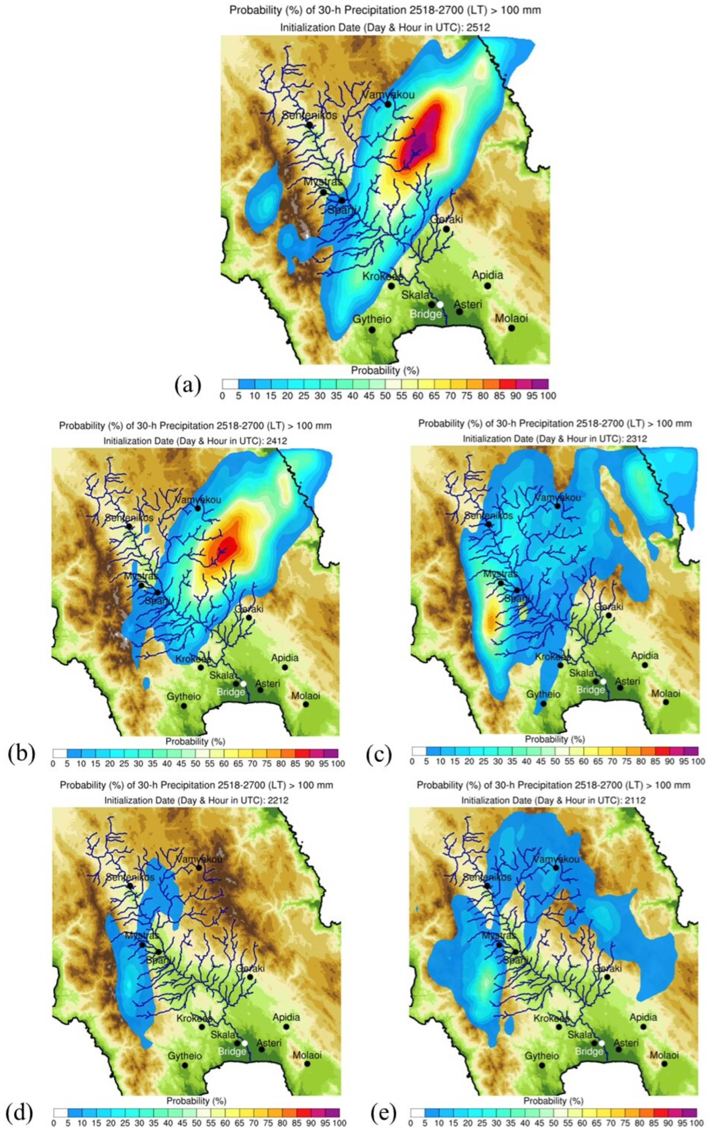
3.2. Probabilistic Forecasting of Precipitation and Discharge at Evrotas River Basin

The deterministic meteorological simulation presented in the previous section (i.e., Oper_0.25 initialized on 25 January at 12:00 UTC) described the atmospheric conditions during the flash flood quite well. However, deterministic simulations, as in our case study, often exhibit inaccuracies. This necessitates adopting a probabilistic approach in precipitation forecasting by using ensemble modelling, which subsequently determines the flash-flood forecast. Thus, this section presents the results of the probabilistic approach followed in this study.

Figure 10a–e demonstrates the spatial distribution of the probability that the predicted 30-h accumulated precipitation (i.e., from 25 January at 18:00 LT to 27 January at 00:00 LT) has exceeded 100 mm. These maps were based on the results of the 33 ensemble simulations (i.e., Oper_0.25, Oper_0.50, Ctrl and Ens1-30) for each initialization date (i.e., 21–25 January at 12:00 UTC), respectively (Figure 10a–e). It is noteworthy that the precipitation accumulation period of 30 h was chosen instead of 24 h in order to consider the precipitation probabilities over a longer time window. This is important especially for the simulations that were initialized 2 and more days before the flood. In this way, it is feasible to unravel flooding signals more clearly even 2–5 days in advance. Figure 10a–e demonstrates that the probabilities for precipitation forecasts exceeding 100 mm are higher 1 and 2 days ahead than 3–5 days ahead the flood. The precipitation forecasts that were initialized on 25 and 24 January at 12:00 UTC (Figure 10a–b) show increased probabilities (exceeding 100 mm) even above 90% and 80%, respectively, in the east of the ERB. The probabilities of exceeding 100 mm in the precipitation forecasts initialized on 23, 22 and 21 January at 12:00 (Figure 10c–e) are smaller and show a smoother spatial distribution and, instead, appear in the western ERB. It is important to note that probabilities reaching even 40–50% can be considered as a sufficient signal of heavy precipitation even 5 days prior the flood, despite some spatial variations. The amount of 100 mm is an indicative precipitation limit that was selected in this study by considering a previous flash flood at the ERB in 2016 [37].

Then, these probabilistic precipitation forecasts were used to force the respective probabilistic hydrological simulations. Figure 11a shows that the probability of discharge exceeding 300 m³ s⁻¹ reached even 80–90% in the main part of the Evrotas river, based on the 33 ensemble hydrological simulations initialized on 25 January at 12:00 UTC. The respective probabilities for the simulations initialized on 24 January at 12:00 UTC (Figure 11b) had peaks of 70–80%, while they reached 50–70% for initializations on 23, 22 and 21 January at 12:00 UTC (Figure 11c–e). Similar to the precipitation limit, the discharge limit of 300 m³ s⁻¹ is an indicative value of high flow that could potentially cause local water level increase, again based on the simulation of 2016 flash flood at the ERB [37]. It is emphasized that the assessment of exceedance of precipitation and discharge limits from some ensemble simulations as presented above, does not necessarily imply the occurrence of flash flood, but indicates the development of favourable conditions and the increase of flood risk.

It is interesting to examine precipitation and discharge together in timeseries (i.e., through hydrographs). Figure 12a–e demonstrates hydrographs for all simulations that were initialized on 25, 24, 23, 22 and 21 January at 12:00 UTC, respectively. In particular, Figure 12 shows how the 1-h areal precipitation, which refers to the total extent of the ERB and the discharge at the Skala’s bridge, changes over time. As expected, the discharge increase presents a lag in comparison with the respective increase in precipitation, as illustrated in Figure 12. The main difference between the hydrographs is the existence of two discharge peaks at noon and late afternoon, as shown in Figure 12a,b, and 1 discharge peak at afternoon, morning and noon, as shown in Figure 12c–e, respectively. The spread of the ensemble precipitation and discharge timeseries is larger for the simulations initialized 2 or more days before the flood, indicating greater uncertainty as the forecasting horizon increases.

This is reasonable and confirms the reliability of the model, as forecasts made in advance, such as 5 days before the flood, exhibit more uncertainty compared to forecasts made closer to the event, as in 2 days before the flood. This can be useful for informing the authorities with gradually increasing ‘certainty’ as an extreme event develops.

This finding is also corroborated by Figure 13a–d, which shows box plots of the 30-h areal precipitation, covering the period from 25 January at 18:00 UTC to 27 January at 00:00 UTC, based on the five different ensemble simulations.

The estimated precipitation and discharge for the 24th and the 25th of January exhibit smaller ranges of values, for all plots of Figure 13. This shows the model’s ability to reduce the temporal uncertainty associated with longer-term forecasts. The use of ensemble forecasting enabled us to both recognize and quantify this uncertainty by exploring multiple possible scenarios, which is a significant strength of this approach.

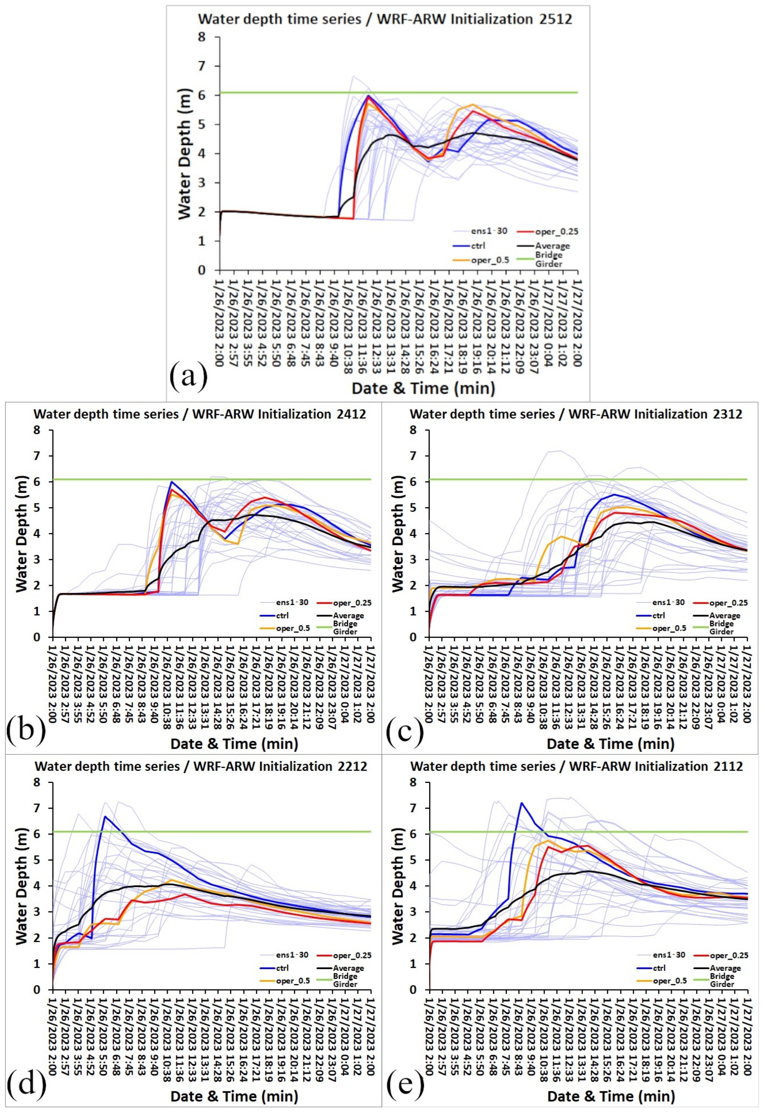
3.3. Probabilistic Forecasting of Water Level at Skala’s Bridge

Finally, the results presented in Figure 11 and Figure 12 (i.e., the hydrographs) were used as inputs for the hydraulic–hydrodynamic model. Thus, following the procedure described in Section 2.5, HEC–RAS produced the flash flooding probabilities for the study area (i.e., Skala’s bridge).

In particular, the spread of water depth obtained from the five different ensemble simulations are shown indicatively for 26 January 2023 in Figure 14. The different water depths are illustrated, as they change over time during the day of the flood event. The horizontal green line represents the height above ground of the Skala bridge’s girder. Similar to the atmospheric and hydrologic results, it is evident that the spread of the different forecasted water depths is larger for the ensemble simulations initialized on the 21 January and becomes smaller in every ensemble simulation initialized closer to 25 January.

This effect of reduced temporal uncertainty in the hydraulic model’s result that follows the hydrologic results is also evident in the water depths at the location of the bridge (Figure 15). Based on the probabilistic hydraulic simulations, the time-variable water depth for the 5-day forecast shows increased probabilities (exceeding 6 m) of 6%, 18%, and 36% for 25 January, 24–22 January, and 21 January 2023, respectively. The lower the probability of exceeding 6 m, the closer the results are to the observed ones.

In Figure 15, the horizontal green line represents the Skala bridge’s girder. The terrain profile line is the actual cross-section at the bridge location, as simulated in HEC–RAS. As shown in Figure 6b, the water level peak at the Skala’s bridge reached 6 m, and all the simulation initializations produced a 6 m-water depth approximately. The results of the maximum water depths were estimated based on the pixel with the maximum water depth along the profile line (as in Figure 5a)

The uncertainty range of the different forecasted maximum water depths is larger for the ensemble initialized on the 21st and becomes smaller in every ensemble initialized closer to the 25 January. In particular, the maximum water depth at Skala Bridge (upstream) shows increased probabilities (exceeding 6 m) of 15%, 18%, 21%, and 36% for 25 January, 24 January, 23–22 January, and 21 January 2023 respectively. This effect can be also observed in the respective box-plots of Figure 16, with the significant reduction of the uncertainty range in the last two days of the initialization of simulations. This underscores the consistency of the uncertainty reduction, as the initializations approach the date of the event, in the same way as in the previous stages of the model.

However, even in the earlier ensemble predictions, the resulting water depths offer valuable insights (in terms of warning signals) into the anticipated severity of the upcoming phenomenon.

4. Conclusions

This study attempted to contribute to efforts towards more accurate predictions of heavy rainfall events that are likely to cause flash floods, by incorporating ensemble weather forecasting into a comprehensive weather-hydrological-hydraulic modeling system (IMBRIW’s system). In particular, this ensemble forecasting process involved multiple simulations, adopting a probabilistic approach based on 33 different initial and boundary condition datasets initialized from one to five days before the observed flood on 26 January 2023, in the ERB. The integrated ensemble weather-hydrological-hydraulic modelling system allowed us to assess the uncertainty in flood forecasts and its potential reduction, providing improved and timely emergency alerts. This capability was showcased at a fine scale, considering specific infrastructure, such as the Skala bridge.

In particular, the ensemble approach provided a range of different precipitation (in mm of water), river discharges (m³ s⁻¹ of water), and flood depths (m of water). These ranges reflect the inherent uncertainties in predictions, demonstrating a consistent pattern based on the timing of model initialization. Notably, greater uncertainty was observed 5 days before the event, gradually narrowing to a more confined range approximately 2–3 days before the observed flood on 26 January. In essence, a more refined indication regarding the impending flood was achieved around 2–3 days before the event (and even more accurate 1–2 days before).

The results obtained from IMBRIW’s system consistently portray the progression from storm conditions to streamflow and, ultimately, water depths at the bridge location. As mentioned, the ensemble precipitation forecasts produced probabilities reaching even 40–50% that can be considered as a sufficient signal of heavy rainfall even 5 days before the flood. So, firstly, it is feasible to receive flooding signals 2–5 days before the event. Subsequently, the forecasted probabilities of discharge exceeding 300 m³ s⁻¹ were considerably high (above 70% in the main part of the river), showing also the discharge peaks over time. Due to the lack of conventional data and records that would facilitate a detailed validation of flood characteristics related to the event on 26 January, the primary criterion for comparing the hydraulic simulations was the estimated flood water depth at the specific location of Skala bridge, as observed from relevant photographs and press documentation. The spread of temporal uncertainties of water depth simulations also narrows for the model initializations of the 2 days before the event. Again, a coherent indication emerges that the approaching storm has the potential to trigger a flood event (i.e., the bridge’s overflow), with a notable convergence in result uncertainties during the final 1–2 days leading up to the event.

This is an advantage of the probabilistic approach over the existing (often used) deterministic approaches. A deterministic approach might have resulted in one of the many different predicted outcomes, signaling either a mild or a very extreme event, depending on its initial and boundary conditions. This is evident at the scale of an infrastructure element, like the bridge in our example (Figure 14 and Figure 15), where the water depths are compared to its girder, so even centimeters can lead to a different perception of risk regarding the bridge’s overflow. The probabilistic forecast of the ensemble approach presented, has the ability to account for these uncertainties and quantify them, while showing their variability over time. By understanding the likelihood of various scenarios (e.g., as depicted in our results), decision makers can have a more comprehensive assessment of risk, facilitating more informed and adaptive plans for action, compared to the deterministic approaches, where the planning is based on one possible scenario, which may be also misleading. This is crucial in emergency planning, where having a range of possible scenarios is valuable for preparedness. The early indications of the presented approach, even with the increased uncertainty, were able to signal the need for heightened vigilance and potential preparation. Apparently, such increased monitoring, timely warning and response, were not the case for the studied event at Skala’s bridge (vehicles were crossing the bridge with water reaching its girder, e.g., Figure 2, and there are no conventional or official estimates of the exact maximum water depth). This shows the value of the early alerting capability that the presented ensemble approach provided, which can be crucial for emergency response planning in the future, including the effective communication of these forecasts regarding upcoming risks to the public. In the case of Skala, it is still unclear when the bridge closed, and how timely this decision and response was. But if this happens in a timely manner, using gradually warnings of increased accuracy (in line with our results), it gives time to become better prepared.

Future research could leverage the current work towards a more holistic approach by incorporating social and economic factors, thereby enhancing the comprehensive understanding and application of the developed flash-flood forecast modeling. A limitation of this ensemble approach could be its computationally demanding nature, although the ongoing advancements in computer and computational sciences provide means to overcome it. Another caveat for adopting such forecasting systems is the limited capacity of the decision makers to utilize and interpret this information effectively, including its communication to the public. However, the importance of building resilient societies in the view of increasing extreme phenomena, and in particular when they involve flash flood predictions that directly threaten human lives and property, highlights the need for capacity building. As scientists make continuous efforts in providing improved methods of conveying uncertainty and probability in ways that can be easily understood and actionable, decision makers should also recognize the need for improved understanding and training to enable informed decision making, and scientifically supported emergency planning.

References

1. Blöschl, G.; Hall, J.; Viglione, A.; Perdigão, R.A.P.; Parajka, J.; Merz, B.; Lun, D.; Arheimer, B.; Aronica, G.T.; Bilibashi, A.; et al. Changing Climate Both Increases and Decreases European River Floods. Nature 2019, 573, 108–111. [Google Scholar] [CrossRef] [PubMed]
2. Berghuijs, W.R.; Aalbers, E.E.; Larsen, J.R.; Trancoso, R.; Woods, R.A. Recent Changes in Extreme Floods across Multiple Continents. Environ. Res. Lett. 2017, 12, 114035. [Google Scholar] [CrossRef]
3. Sanders, B.F.; Schubert, J.E.; Kahl, D.T.; Mach, K.J.; Brady, D.; AghaKouchak, A.; Forman, F.; Matthew, R.A.; Ulibarri, N.; Davis, S.J. Large and Inequitable Flood Risks in Los Angeles, California. Nat. Sustain. 2023, 6, 47–57. [Google Scholar] [CrossRef]
4. Johnson, K.A.; Wing, O.E.J.; Bates, P.D.; Fargione, J.; Kroeger, T.; Larson, W.D.; Sampson, C.C.; Smith, A.M. A Benefit–Cost Analysis of Floodplain Land Acquisition for US Flood Damage Reduction. Nat. Sustain. 2020, 3, 56–62. [Google Scholar] [CrossRef]
5. Cloke, H.L.; Pappenberger, F. Ensemble Flood Forecasting: A Review. J. Hydrol. 2009, 375, 613–626. [Google Scholar] [CrossRef]
6. Maidment, D.R. Conceptual Framework for the National Flood Interoperability Experiment. J. Am. Water Resour. Assoc. 2017, 53, 245–257. [Google Scholar] [CrossRef]
7. Giannaros, C.; Galanaki, E.; Kotroni, V.; Lagouvardos, K.; Oikonomou, C.; Haralambous, H.; Giannaros, T.M. Pre-Operational Application of a WRF-Hydro-Based Fluvial Flood Forecasting System in the Southeast Mediterranean. Forecasting 2021, 3, 437–446. [Google Scholar] [CrossRef]
8. Ahmad, T.; Pandey, A.; Kumar, A. Evaluating Urban Growth and Its Implication on Flood Hazard and Vulnerability in Srinagar City, Kashmir Valley, Using Geoinformatics. Arab. J. Geosci. 2019, 12, 308. [Google Scholar] [CrossRef]
9. Alamanos, A.; Linnane, S. Systems Resilience to Floods: A Categorisation of Approaches. In Proceedings of the 24th EGU General Assembly, Vienna, Austria, 23–27 May 2022. [Google Scholar]
10. Papaioannou, G.; Alamanos, A.; Maris, F. Evaluating Post-Fire Erosion and Flood Protection Techniques: A Narrative Review of Applications. GeoHazards 2023, 4, 380–405. [Google Scholar] [CrossRef]
11. Flageollet, J.-C. Landslide Hazard—A Conceptual Approach in Risk Viewpoint. In Floods and Landslides: Integrated Risk Assessment; Casale, R., Margottini, C., Eds.; Environmental Science; Springer: Berlin, Germany, 1999; pp. 3–18. ISBN 978-3-642-58609-5. [Google Scholar]
12. Kouwen, N. WATFLOOD: A Micro-Computer Based Flood Forecasting System Based on Real-Time Weather Radar. Can. Water Resour. J. 1988, 13, 62–77. [Google Scholar] [CrossRef]
13. Bogardi, J.J.; Kundzewicz, Z.W. Risk, Reliability, Uncertainty, and Robustness of Water Resource Systems; Cambridge University Press: Cambridge, UK, 2002; ISBN 978-1-139-43224-5. [Google Scholar]
14. Rossa, A.; Liechti, K.; Zappa, M.; Bruen, M.; Germann, U.; Haase, G.; Keil, C.; Krahe, P. The COST 731 Action: A Review on Uncertainty Propagation in Advanced Hydro-Meteorological Forecast Systems. Atmos. Res. 2011, 100, 150–167. [Google Scholar] [CrossRef]
15. Alamanos, A.; Linnane, S. Drought Monitoring, Precipitation Statistics, and Water Balance with Freely Available Remote Sensing Data: Examples, Advances, and Limitations. In Proceedings of the Irish National Hydrology Conference 2021, Athlone, Ireland, 16 November 2021; pp. 1–13. [Google Scholar]
16. Alamanos, A. Water Resources Planning under Climate and Economic Changes in Skiathos Island, Aegean. Water Infrastruct. Ecosyst. Soc. 2021, 70, 1085–1093. [Google Scholar] [CrossRef]
17. Adams, T.E. Chapter 10—Flood Forecasting in the United States NOAA/National Weather Service. In Flood Forecasting; Adams, T.E., Pagano, T.C., Eds.; Academic Press: Boston, MA, USA, 2016; pp. 249–310. ISBN 978-0-12-801884-2. [Google Scholar]
18. Wu, W.; Emerton, R.; Duan, Q.; Wood, A.W.; Wetterhall, F.; Robertson, D.E. Ensemble Flood Forecasting: Current Status and Future Opportunities. WIREs Water 2020, 7, e1432. [Google Scholar] [CrossRef]
19. Alamanos, A. Sustainable Water Resources Management under Water-Scarce and Limited-Data Conditions. Cent. Asian J. Water Res. 2021, 7, 1–19. [Google Scholar] [CrossRef]
20. Hansen, J.W.; Dinku, T.; Robertson, A.W.; Cousin, R.; Trzaska, S.; Mason, S.J. Flexible Forecast Presentation Overcomes Longstanding Obstacles to Using Probabilistic Seasonal Forecasts. Front. Clim. 2022, 4, 908661. [Google Scholar] [CrossRef]
21. Han, S.; Coulibaly, P. Probabilistic Flood Forecasting Using Hydrologic Uncertainty Processor with Ensemble Weather Forecasts. J. Hydrometeorol. 2019, 20, 1379–1398. [Google Scholar] [CrossRef]
22. Todini, E. Flood Forecasting and Decision Making in the New Millennium. Where Are We? Water Resour. Manag. 2017, 31, 3111–3129. [Google Scholar] [CrossRef]
23. Krajewski, W.F.; Ceynar, D.; Demir, I.; Goska, R.; Kruger, A.; Langel, C.; Mantilla, R.; Niemeier, J.; Quintero, F.; Seo, B.-C.; et al. Real-Time Flood Forecasting and Information System for the State of Iowa. Bull. Am. Meteorol. Soc. 2017, 98, 539–554. [Google Scholar] [CrossRef]
24. Marty, R.; Zin, I.; Obled, C. Sensitivity of Hydrological Ensemble Forecasts to Different Sources and Temporal Resolutions of Probabilistic Quantitative Precipitation Forecasts: Flash Flood Case Studies in the Cévennes-Vivarais Region (Southern France). Hydrol. Process. 2013, 27, 33–44. [Google Scholar] [CrossRef]
25. Goodarzi, L.; Banihabib, M.E.; Roozbahani, A. A Decision-Making Model for Flood Warning System Based on Ensemble Forecasts. J. Hydrol. 2019, 573, 207–219. [Google Scholar] [CrossRef]
26. Ramos, M.-H.; Bartholmes, J.; Thielen-del Pozo, J. Development of Decision Support Products Based on Ensemble Forecasts in the European Flood Alert System. Atmos. Sci. Lett. 2007, 8, 113–119. [Google Scholar] [CrossRef]
27. Ming, X.; Liang, Q.; Xia, X.; Li, D.; Fowler, H.J. Real-Time Flood Forecasting Based on a High-Performance 2-D Hydrodynamic Model and Numerical Weather Predictions. Water Resour. Res. 2020, 56, e2019WR025583. [Google Scholar] [CrossRef]
28. Richardson, D.; Neal, R.; Dankers, R.; Mylne, K.; Cowling, R.; Clements, H.; Millard, J. Linking Weather Patterns to Regional Extreme Precipitation for Highlighting Potential Flood Events in Medium- to Long-Range Forecasts. Meteorol. Appl. 2020, 27, e1931. [Google Scholar] [CrossRef]
29. Nanditha, J.S.; Mishra, V. On the Need of Ensemble Flood Forecast in India. Water Secur. 2021, 12, 100086. [Google Scholar] [CrossRef]
30. Gude, V.; Corns, S.; Long, S. Flood Prediction and Uncertainty Estimation Using Deep Learning. Water 2020, 12, 884. [Google Scholar] [CrossRef]
31. Alamanos, A.; Papaioannou, G.; Varlas, G.; Markogianni, V.; Papadopoulos, A.; Dimitriou, E. Representation of a Post-Fire Flash-Flood Event Combining Meteorological Simulations, Remote Sensing, and Hydraulic Modeling. Land 2024, 13, 47. [Google Scholar] [CrossRef]
32. Galia, T.; Macurová, T.; Vardakas, L.; Škarpich, V.; Matušková, T.; Kalogianni, E. Drivers of Variability in Large Wood Loads along the Fluvial Continuum of a Mediterranean Intermittent River. Earth Surf. Process. Landf. 2020, 45, 2048–2062. [Google Scholar] [CrossRef]
33. Matiatos, I.; Papadopoulos, A.; Panagopoulos, Y.; Dimitriou, E. Insights into the Influence of Morphology on the Hydrological Processes of River Catchments Using Stable Isotopes. Hydrol. Sci. J. 2023, 68, 1487–1498. [Google Scholar] [CrossRef]
34. Karaouzas, I.; Theodoropoulos, C.; Vardakas, L.; Zogaris, S.; Skoulikidis, N. Theodoropoulos, C.; Vardakas, L.; Zogaris, S.; Skoulikidis, N. The Evrotas River Basin: 10 Years of Ecological Monitoring. In The Rivers of Greece: Evolution, Current Status and Perspectives; Skoulikidis, N., Dimitriou, E., Karaouzas, I., Eds.; The Handbook of Environmental Chemistry; Springer: Berlin, Germany, 2018; pp. 279–326. ISBN 978-3-662-55369-5. [Google Scholar]
35. Galia, T.; Škarpich, V.; Vardakas, L.; Dimitriou, E.; Panagopoulos, Y.; Spálovský, V. Spatiotemporal Variations of Large Wood and River Channel Morphology in a Rapidly Degraded Reach of an Intermittent River. Earth Surf. Process. Landf. 2023, 48, 997–1010. [Google Scholar] [CrossRef]
36. Tzoraki, O.; Cooper, D.; Kjeldsen, T.; Nikolaidis, N.P.; Gamvroudis, C.; Froebrich, J.; Querner, E.; Gallart, F.; Karalemas, N. Flood Generation and Classification of a Semi-Arid Intermittent Flow Watershed: Evrotas River. Int. J. River Basin Manag. 2013, 11, 77–92. [Google Scholar] [CrossRef]
37. Varlas, G.; Papadopoulos, A.; Papaioannou, G.; Dimitriou, E. Evaluating the Forecast Skill of a Hydrometeorological Modelling System in Greece. Atmosphere 2021, 12, 902. [Google Scholar] [CrossRef]
38. SKAI News Dangerous Rise of Evrotas River Water Levels. Available online: https://www.skai.gr/news/greece/anevainei-epikindyna-i-stathmi-tou-potamou-eyrota-deite-vinteo (accessed on 17 November 2023).
39. The TOC Storms in Lakonia: Floods, Damages and Closed Roads in Evrotas Municipality. Available online: https://www.thetoc.gr/koinwnia/article/sto-eleos-tis-kakokairias-i-lakonia-plimmures-adiabatoi-dromoi-kai-zimies-ston-dimo-eurota-eikones/ (accessed on 17 November 2023).
40. Skamarock, C.; Klemp, B.; Dudhia, J.; Gill, O.; Barker, D.; Duda, G.; Huang, X.; Wang, W.; Powers, G. A Description of the Advanced Research WRF Version 3. NCAR Tech. Note 2008, 475, 113. [Google Scholar] [CrossRef]
41. Gochis, D.; Yu, W.; Yates, D. WRF-Hydro Technical Description and User’s Guide; The NCAR WRF-Hydro Technical Description and User’s Guide; NCAR: Boulder, CO, USA, 2015; p. 120. [Google Scholar]
42. Hydrologic Engineering Center (HEC) River Analysis Systems—HEC-RAS, version 6.3.1; U.S. Army Corps of Engineers: Washington, DC, USA, 2022.
43. Skamarock, C.; Klemp, B.; Dudhia, J.; Gill, O.; Liu, Z.; Berner, J.; Wang, W.; Powers, G.; Duda, G.; Barker, D.; et al. A Description of the Advanced Research WRF Model Version 4.3; No. NCAR/TN-556+STR; NSF: Alexandria, VI, USA, 2021. [Google Scholar] [CrossRef]
44. Danielson, J.; Gesch, D. Global Multi-Resolution Terrain Elevation Data 2010 (GMTED2010); 211AD; USGS: Reston, VA, USA, 2011; p. 34. [Google Scholar]
45. Myneni, R.B.; Hoffman, S.; Knyazikhin, Y.; Privette, J.L.; Glassy, J.; Tian, Y.; Wang, Y.; Song, X.; Zhang, Y.; Smith, G.R.; et al. Global Products of Vegetation Leaf Area and Fraction Absorbed PAR from Year One of MODIS Data. Remote Sens. Environ. 2002, 83, 214–231. [Google Scholar] [CrossRef]
46. Friedl, M.A.; Sulla-Menashe, D.; Tan, B.; Schneider, A.; Ramankutty, N.; Sibley, A.; Huang, X. MODIS Collection 5 Global Land Cover: Algorithm Refinements and Characterization of New Datasets. Remote Sens. Environ. 2010, 114, 168–182. [Google Scholar] [CrossRef]
47. Jiménez, P.A.; Dudhia, J.; González-Rouco, J.F.; Navarro, J.; Montávez, J.P.; García-Bustamante, E. A Revised Scheme for the WRF Surface Layer Formulation. Mon. Weather. Rev. 2012, 140, 898–918. [Google Scholar] [CrossRef]
48. Nakanishi, M.; Niino, H. Development of an Improved Turbulence Closure Model for the Atmospheric Boundary Layer. J. Meteorol. Soc. Jpn. Ser. II 2009, 87, 895–912. [Google Scholar] [CrossRef]
49. Tewari, M.; Boulder, C.; Chen, F.; Wang, W.; Dudhia, J.; LeMone, M.; Mitchell, K.; Ek, M.; Gayno, G.; Wegiel, J.; et al. Implementation and Verification of the Unified Noah Land Surface Model in the WRF Model. In Proceedings of the 20th Conference on Weather Analysis and Forecasting/16th Conference on Numerical Weather Prediction, Seattle, DC, USA, 12–16 January 2004. Volume Formerly Paper Number 17.5. [Google Scholar]
50. Iacono, M.J.; Delamere, J.S.; Mlawer, E.J.; Shephard, M.W.; Clough, S.A.; Collins, W.D. Radiative Forcing by Long-Lived Greenhouse Gases: Calculations with the AER Radiative Transfer Models. J. Geophys. Res. Atmos. 2008, 113, D13. [Google Scholar] [CrossRef]
51. Chen, S.-H.; Sun, W.-Y. A One-Dimensional Time Dependent Cloud Model. J. Meteorol. Soc. Jpn. Ser. II 2002, 80, 99–118. [Google Scholar] [CrossRef]
52. Grell, G.A.; Freitas, S.R. A Scale and Aerosol Aware Stochastic Convective Parameterization for Weather and Air Quality Modeling. Atmos. Chem. Phys. 2014, 14, 5233–5250. [Google Scholar] [CrossRef]
53. Ek, M.B.; Mitchell, K.E.; Lin, Y.; Rogers, E.; Grunmann, P.; Koren, V.; Gayno, G.; Tarpley, J.D. Implementation of Noah Land Surface Model Advances in the National Centers for Environmental Prediction Operational Mesoscale Eta Model. J. Geophys. Res. Atmos. 2003, 108, D22. [Google Scholar] [CrossRef]
54. Julien, P.Y.; Saghafian, B.; Ogden, F.L. Raster-Based Hydrologic Modeling of Spatially-Varied Surface Runoff1. J. Am. Water Resour. Assoc. 1995, 31, 523–536. [Google Scholar] [CrossRef]
55. Ogden, F. CASC2D Reference Manual; University of Connecticut: Storrs, CT, USA, 1997. [Google Scholar]
56. Garbrecht, J.; Brunner, G. Hydrologic Channel-Flow Routing for Compound Sections. J. Hydraul. Eng. 1991, 117, 629–642. [Google Scholar] [CrossRef]
57. Jarvis, A.; Guevara, E.; Reuter, H.I.; Nelson, A.D. Hole-Filled SRTM for the Globe: Version 4: Data Grid; University of Twente: Enschede, The Netherlands, 2008. [Google Scholar]
58. Lehner, B.; Verdin, K.; Jarvis, A. New Global Hydrography Derived from Spaceborne Elevation Data. EOS Trans. Am. Geophys. Union 2008, 89, 93–94. [Google Scholar] [CrossRef]
59. HydroSHEDS. Available online: https://www.hydrosheds.org/ (accessed on 17 November 2023).
60. Strahler, A.N. Hypsometric (area-altitude) analysis of erosional topography. GSA Bull. 1952, 63, 1117–1142. [Google Scholar] [CrossRef]
61. Varlas, G.; Anagnostou, M.N.; Spyrou, C.; Papadopoulos, A.; Kalogiros, J.; Mentzafou, A.; Michaelides, S.; Baltas, E.; Karymbalis, E.; Katsafados, P. A Multi-Platform Hydrometeorological Analysis of the Flash Flood Event of 15 November 2017 in Attica, Greece. Remote Sens. 2019, 11, 45. [Google Scholar] [CrossRef]
62. Papaioannou, G.; Varlas, G.; Papadopoulos, A.; Loukas, A.; Katsafados, P.; Dimitriou, E. Investigating Sea-State Effects on Flash Flood Hydrograph and Inundation Forecasting. Hydrol. Process. 2021, 35, e14151. [Google Scholar] [CrossRef]
63. Papaioannou, G.; Varlas, G.; Terti, G.; Papadopoulos, A.; Loukas, A.; Panagopoulos, Y.; Dimitriou, E. Flood Inundation Mapping at Ungauged Basins Using Coupled Hydrometeorological–Hydraulic Modelling: The Catastrophic Case of the 2006 Flash Flood in Volos City, Greece. Water 2019, 11, 2328. [Google Scholar] [CrossRef]
64. Spyrou, C.; Varlas, G.; Pappa, A.; Mentzafou, A.; Katsafados, P.; Papadopoulos, A.; Anagnostou, M.N.; Kalogiros, J. Implementation of a Nowcasting Hydrometeorological System for Studying Flash Flood Events: The Case of Mandra, Greece. Remote Sens. 2020, 12, 2784. [Google Scholar] [CrossRef]
65. Camera, C.; Bruggeman, A.; Zittis, G.; Sofokleous, I.; Arnault, J. Simulation of Extreme Rainfall and Streamflow Events in Small Mediterranean Watersheds with a One-Way-Coupled Atmospheric–Hydrologic Modelling System. Nat. Hazards Earth Syst. Sci. 2020, 20, 2791–2810. [Google Scholar] [CrossRef]
66. Senatore, A.; Furnari, L.; Mendicino, G. Impact of High-Resolution Sea Surface Temperature Representation on the Forecast of Small Mediterranean Catchments’ Hydrological Responses to Heavy Precipitation. Hydrol. Earth Syst. Sci. 2020, 24, 269–291. [Google Scholar] [CrossRef]
67. Yucel, I.; Onen, A.; Yilmaz, K.K.; Gochis, D.J. Calibration and Evaluation of a Flood Forecasting System: Utility of Numerical Weather Prediction Model, Data Assimilation and Satellite-Based Rainfall. J. Hydrol. 2015, 523, 49–66. [Google Scholar] [CrossRef]
68. Ozkaya, A.; Akyurek, Z. WRF-Hydro Model Application in a Data-Scarce, Small and Topographically Steep Catchment in Samsun, Turkey. Arab. J. Sci. Eng. 2020, 45, 3781–3798. [Google Scholar] [CrossRef]
69. Khanam, M.; Sofia, G.; Koukoula, M.; Lazin, R.; Nikolopoulos, E.I.; Shen, X.; Anagnostou, E.N. Impact of Compound Flood Event on Coastal Critical Infrastructures Considering Current and Future Climate. Nat. Hazards Earth Syst. Sci. 2021, 21, 587–605. [Google Scholar] [CrossRef]
70. Urzică, A.; Mihu-Pintilie, A.; Stoleriu, C.C.; Cîmpianu, C.I.; Huţanu, E.; Pricop, C.I.; Grozavu, A. Using 2D HEC-RAS Modeling and Embankment Dam Break Scenario for Assessing the Flood Control Capacity of a Multi-Reservoir System (NE Romania). Water 2021, 13, 57. [Google Scholar] [CrossRef]
71. Psomiadis, E.; Tomanis, L.; Kavvadias, A.; Soulis, K.X.; Charizopoulos, N.; Michas, S. Potential Dam Breach Analysis and Flood Wave Risk Assessment Using HEC-RAS and Remote Sensing Data: A Multicriteria Approach. Water 2021, 13, 364. [Google Scholar] [CrossRef]
72. Papaioannou, G.; Vasiliades, L.; Loukas, A.; Alamanos, A.; Efstratiadis, A.; Koukouvinos, A.; Tsoukalas, I.; Kossieris, P. A Flood Inundation Modeling Approach for Urban and Rural Areas in Lake and Large-Scale River Basins. Water 2021, 13, 1264. [Google Scholar] [CrossRef]
73. Muthusamy, M.; Casado, M.R.; Butler, D.; Leinster, P. Understanding the Effects of Digital Elevation Model Resolution in Urban Fluvial Flood Modelling. J. Hydrol. 2021, 596, 126088. [Google Scholar] [CrossRef]
74. Wang, W.; Yang, X.; Yao, T. Evaluation of ASTER GDEM and SRTM and Their Suitability in Hydraulic Modelling of a Glacial Lake Outburst Flood in Southeast Tibet. Hydrol. Process. 2012, 26, 213–225. [Google Scholar] [CrossRef]
75. Senatore, A.; Mendicino, G.; Gochis, D.J.; Yu, W.; Yates, D.N.; Kunstmann, H. Fully Coupled Atmosphere-Hydrology Simulations for the Central Mediterranean: Impact of Enhanced Hydrological Parameterization for Short and Long Time Scales. J. Adv. Model. Earth Syst. 2015, 7, 1693–1715. [Google Scholar] [CrossRef]
76. Lim, N.J.; Brandt, S.A. Flood Map Boundary Sensitivity Due to Combined Effects of DEM Resolution and Roughness in Relation to Model Performance. Geomat. Nat. Hazards Risk 2019, 10, 1613–1647. [Google Scholar] [CrossRef]
77. Water Special Secretariat, Ministry of Environment and Energy (SSW-MEE). Flood Risk Management Plans of Eastern Peloponnese River Basin District. Flood Risk Maps; Water Special Secretariat, Ministry of Environment and Energy (SSW-MEE): Athens, Greece, 2018. [Google Scholar]
78. Laconialive.gr. Skala’s Bridge “Disappeared.” Laconialive.gr—H ενημερωτική ιστοσελίδα της Λακωνίας, Νέα και ειδήσεις; Laconialive: Sparta, Greece, 2016; Available online: https://laconialive.gr/%CE%B5%CE%BE%CE%B1%CF%86%CE%B1%CE%BD%CE%AF%CF%83%CF%84%CE%B7%CE%BA%CE%B5-%CE%B7-%CE%B3%CE%AD%CF%86%CF%85%CF%81%CE%B1-%CF%84%CE%B7%CF%82-%CF%83%CE%BA%CE%AC%CE%BB%CE%B1%CF%82/ (accessed on 17 November 2023).
79. Güvel, S.; Ali Akgül, M.; Aksu, H. Flood Inundation Maps Using Sentinel-2: A Case Study in Berdan Plain. Water Supply 2022, 22, 4098–4108. [Google Scholar] [CrossRef]
80. Copernicus. The Sentinels Scientific Data Hub. Available online: https://scihub.copernicus.eu/maintenance.html#/home (accessed on 2 February 2023).
81. Xu, H. Modification of Normalised Difference Water Index (NDWI) to Enhance Open Water Features in Remotely Sensed Imagery. Int. J. Remote Sens. 2006, 27, 3025–3033. [Google Scholar] [CrossRef]
82. Notospress. Evrotas Floods. Available online: https://www.notospress.gr/peloponnisos/story/85679/plimmyra-eyrota-megalo-ypsos-vroxis-ena-texniko-ergo-poy-den-egine-kai-mia-meleti-poy-anaklithike (accessed on 17 November 2023).
83. wetter3.de. Available online: https://www1.wetter3.de/ (accessed on 17 November 2023).
Figure 1. The study area, Evrotas river basin (ERB). Skala’s bridge is also shown. The water level of the Evrotas river reached the Skala’s bridge and almost overtopped it.
Atmosphere 15 00120 g001
Figure 2. Pictures from the flood of 26 January 2023 around the Skala location in ERB. Sources: [38,39].
Atmosphere 15 00120 g002
Figure 3. Flowchart illustrating the main data used in simulations and the model setup of the ensemble hydrometeorological–hydraulic forecasting system.
Atmosphere 15 00120 g003
Figure 4. (a) WRF–ARW model domains (D1: 36 km × 36 km, D2: 12 km × 12 km, D3: 4 km × 4 km, and Evrotas: 1 km × 1 km); (b) Topography (m) with horizontal resolution of 100 m × 100 m and stream order (from 2 to 6 orders illustrated) used by the WRF–Hydro model in ERB. Skala’s bridge (white color) and various station locations (blue color) are also depicted.
Atmosphere 15 00120 g004
Figure 5. Hydraulic modelling specifications at Skala’s bridge. (a) Hydraulic model setup in HEC–RAS showing the “Geometry” representation of the study area along with the effect of bridge design in the generation of the computational mesh for the 2D flow simulation. (b) UAV aerial photographs of the study area determining the model’s schematic. (c) Topographical survey sketch including the bridge’s characteristics [77]. (d) Technical details of the bridge piers and abutments, as simulated in HEC–RAS. (e) Topographical survey photographs [77]. (f) Photographs of Skala’s bridge during the flash flood event [38,39].
Atmosphere 15 00120 g005
Figure 7. (a) Geopotential height (black contours in gpdam) and temperature (color-shaded areas and white contours at °C) at the isobaric level of 500 hPa on 26 January 2023 at 00:00 UTC. The map is based on analysis data from the Global Forecast System (GFS). The German word geopotential appearing in the image corresponds to the term geopotential height. Also, the German words temperatur and Donnerstag are temperature and Thursday, respectively; (b) UK Met Office surface analysis map (isobaric contours in hPa) on 26 January 2023 at 00:00 UTC. Source: [83]. The symbols “H” and “L” show barometric highs and lows, while the symbol “T” in (a) shows barometric lows.
Atmosphere 15 00120 g007
Figure 8. 24-h accumulated precipitation (mm) for 26 January 2023 spatially distributed from the 1-km meteorological forecasts. In addition, 24-h accumulated precipitation measurements from meteorological stations (i.e., meteorological stations from IMBRIW-HCMR, NOA and HUA) are depicted next to the station names, while the respective forecasted values are also shown at the right for comparison. Topography (m) is also illustrated as in Figure 4b.
Atmosphere 15 00120 g008
Figure 9. The evolution of the simulated event, for 26 January 2023, in terms of 1-h accumulated precipitation and streams’ discharge, at: (a) 07:00; (b) 08:00; (c) 09:00; (d) 10:00; (e) 11:00; (f) 12:00 (local time—LT). Topography (m) is also illustrated as in Figure 4b.
Atmosphere 15 00120 g009
Figure 10. Probability maps, showing the spatial distribution of the probability of occurrence of a predefined 30-h accumulated precipitation greater than 100 mm, for the 5-day forecast initialized on: (a) 25 January; (b) 24 January; (c) 23 January; (d) 22 January; (e) 21 January 2023 at 12:00 UTC. Topography (m) is also illustrated as in Figure 4b.
Atmosphere 15 00120 g010
Figure 11. Probability maps for the maximum discharge in the study area’s streams, to exceed 300 m3 s−1, for the 5-day forecast: (a) 25 January; (b) 24 January; (c) 23 January; (d) 22 January; (e) 21 January 2023. Topography (m) is also illustrated as in Figure 4b.
Atmosphere 15 00120 g011
Figure 12. Ensemble timeseries of areal precipitation (upper part of the plots) and discharge hydrographs (lower part of the plots), as simulated for the forecasts initialized on: (a) 25 January; (b) 24 January; (c) 23 January; (d) 22 January; (e) 21 January 2023.
Atmosphere 15 00120 g012
Figure 13. The box plots of the ensemble-forecasted simulations: (a) 30-h areal precipitation; (b) 1-h maximum areal precipitation; (c) average discharge at Skala bridge; (d) maximum discharge at Skala bridge, for each forecast initialization date, from 21–25 January 2023.
Atmosphere 15 00120 g013
Figure 14. Time-variable water depth based on the probabilistic hydraulic simulations, for the 5-day forecast initialized on the: (a) 25 January; (b) 24 January; (c) 23 January; (d) 22 January; (e) 21 January 2023.
Atmosphere 15 00120 g014
Figure 15. Maximum water depths at the Skala bridge (upstream) for the 5-day forecast initialized on the: (a) 25 January; (b) 24 January; (c) 23 January; (d) 22 January; (e) 21 January 2023.
Atmosphere 15 00120 g015
Figure 16. Box-plots of the ensemble-forecasted simulation results of the maximum water depths based on the time-variable water depth results, for each initialization date (21–25 January).
Atmosphere 15 00120 g016