Article

Trace Elements Concentrations in Urban Air in Helsinki, Finland during a 44-Year Period

by
Eleftheria Ioannidou
1,*,
Stefanos Papagiannis
2,3,4,
Manousos Ioannis Manousakas
2,5,
Chrysoula Betsou
1,6,
Konstantinos Eleftheriadis
2,
Jussi Paatero
7,
Lambrini Papadopoulou
8 and
Alexandra Ioannidou
1
1
Nuclear Physics & Elementary Particle Physics Division, School of Physics, Aristotle University of Thessaloniki, 54124 Thessaloniki, Greece
2
Environmental Radioactivity Laboratory, INRASTES, NCSR Demokritos, Agia Paraskevi, 15310 Athens, Greece
3
Department of Materials Science and Engineering, University of Ioannina, 45110 Ioannina, Greece
4
Institute of Nuclear and Particle Physics, NCSR Demokritos, Agia Paraskevi, 15310 Athens, Greece
5
Laboratory of Atmospheric Chemistry, Paul Scherrer Institute, 5232 Villigen, Switzerland
6
Laboratory of Archaeometry and Physicochemical Measurements, ATHENA-Research and Innovation Centre, 67100 Xanthi, Greece
7
Finnish Meteorological Institute (FMI), Observation Services, P.O. Box 503, FI-00101 Helsinki, Finland
8
Department of Mineralogy-Petrology-Economic Geology, School of Geology, Aristotle University of Thessaloniki, 54124 Thessaloniki, Greece
*
Author to whom correspondence should be addressed.
Atmosphere 2023, 14(9), 1430; https://doi.org/10.3390/atmos14091430
Submission received: 19 July 2023 / Revised: 7 September 2023 / Accepted: 11 September 2023 / Published: 13 September 2023

Abstract

:
The atmospheric concentrations of seventeen elements were measured in air filters at the Finnish Meteorological Institute station in Helsinki, Finland, during a period of 44 years (1962–2005). The mean annual concentrations were calculated and are presented from the lowest values to the highest ones Cr < Ni < Ti < Br < V < Mn < Cu < Zn < Cl < Al < Fe < K < Ca < Na < Pb < Si < S. Most of the elements (Fe, Si, Ti, K, Ca, Zn, Br, Pb, V, Ni, S, Cr, Na, Al, and Cl) present higher values during spring and winter season, while in summer the elements (Ti, Ca, S, and Na) are found in higher concentrationsdue to the weather conditions across seasons and the sources and emissions of air pollutants. There is a strong correlation between the elements (V-Ni, Si-Pb, Fe-Ca, V-Cr, Si-K, K-Ca, Fe-Ti, K-Na, Si-Ca, and V-S), indicating their common source. The identification of the sources of trace elements was performed based on positive matrix factorization analysis, using SoFi software. Four Suspended Particulate Matter (PM) sources were identified: road dust (due to usage of leaded fuel), heavy oil combustion/secondary sulfates, traffic emissions, and natural dust (soil). For the total of 44 years studied, significant decreases in concentrations were observed for all elements, most of which were over 50%: Na (−74%), Al (−86%), Si (−88%), S (−82%), K (−82%), Ca (−89%), Ti (−80%), V (−89%), Cr (−82%), Mn (−77%), Fe (−77%), Ni (−61%), Zn (−72%), and Pb (−95%). In general, a significant decline has been observed in the majority of the elemental concentrations since the end of the 1970s, underlying the effectiveness of different environmental policies that have been applied during the last few decades.

1. Introduction

Air pollution is an environmental and human health issue that continuously concerns worldwide [1]. Suspended Particulate Matter (PM) is an important atmospheric pollutant with severe public health effects, particularly in metropolitan areas that are heavily affected by emissions from vehicles, industry, and other sources of urban pollution [2,3,4,5]. Inhalable particulate matter refers to particles with a diameter less than 10 μm. These particles have a complex composition, including organic substances, inorganic salts, and heavy metals. They have the ability to accumulate in the lungs, leading to health issues such as asthma, arrhythmia, and bronchitis, which can even result in increased mortality rates. Between 1990 and 2019, worldwide deaths due to air pollution rose by 2.62%. Furthermore, over 90% of the global population resides in areas not meeting air quality standards established by the WHO [6,7]. Different studies have correlated particles with severe respiratory diseases, such as lung cancer, and chronic obstructive pulmonary disease [4,5,8,9,10], as well as with cardiovascular diseases such as stroke, deep vein thrombosis, coronary events, myocardial infractions, atherosclerosis [8,9], and with other physical and mental health disorders [11,12,13]. In order to fully understand the impact of particles on human health and the environment, a comprehensive characterization of the atmospheric aerosol is needed.
Aerosol particles are a complex mixture of chemical species coming from different sources, either anthropogenic (traffic, industry, and combustion processes in general) or natural (seasalt, wind-blow dust, forest fires, and volcanic eruptions) [14]. For example, the resuspended soil dust contributes to the total emission of specific trace elements (e.g., Cr, Mn, V, and Ni) to the atmosphere [15]. Some elements like As, Cd, and Ni are linked with both natural and anthropogenic sources [16]. Some of them are released into the atmosphere through the combustion of fossil fuels for the production of heat and electricity (e.g., As, Cd, Cr, Mn, Ni, and V), on non-ferrous metal production (e.g., As, Cd, Cu, and Zn) [4,17] and of waste incineration (As, Cl, Cd, Co, Cu, Cr, Mo, Ni, Pb, and Zn) [18,19]. The atmospheric elements Pb, Fe, Cu, Ni, and Cd are usually emitted due to traffic while Zn comes from vehicle tire rubber abrasion [15]. Leaded gasoline combustion was considered to be traditionally the major source of Pb [17], but nowadays the industrial processes and the energy sector are responsible for most of the Pb emissions in Europe [20]. In the EU, road transport still generates 20% of Pb emissions, as the residual Pb in fuel, engine lubricants, and parts, as well as tires and breaks, still contribute to the emissions [20]. The elemental content of the aerosol particles and their association with different sources is crucial, especially for environmental legislation, showing that future efforts need to be focused on specific sources in order to be successful and effective [15,21].
There are several factors that affect the aerosol’s characteristics and their deposition to the ecosystem even at distances far away from their source, like the particle size, speed, and temperature of exhaust fumes, the height of release, prevailing winds, precipitation conditions, topography, and soil cover [22,23]. A lot of trace elements in particles are also influenced by long-range transport, giving the advantage of identifying even distant sources just by knowing the elemental composition of the particles. Thus, trace elements can be used as tracers of possible transports of atmospheric pollutants even at far distances [15,24].
In Europe, during the last few decades, a declining trend has been observed in the majority of trace element concentrations but there is still a potential for further reduction [4,15,25]. From 1990 to 2017, the emissions of Cd, Pb, and Hg have decreased by 64%, 93%, and 72%, respectively, while in Finland, Cd has been reduced by 86%, Pb by 95%, and Hg by 47% [20]. Since the beginning of the 20th century and the beginning of the 21st century, the EU has established different directives (e.g., Directives 92/72/EEC, 96/62/EC, 1999/30/EC, 2000/69/EC, 2002/3/EC) in order to reduce air pollution to levels that minimize harmful effects on human health and the environment as a whole and have, thus, set limits and target values for different elemental concentrations in aerosols (e.g., As, Cd, Ni, and Pb) [26,27,28,29] as well as in sulfur and other organic compounds. Different national inventories have been established for tracking possible pollution emission sources and the emitted quantities such as EMEP (European Monitoring and Evaluation Program), NEI (National Emissions Inventory, USA), and NPRI (National Pollutant Release Inventories; Canada) [30].
In Finland, studies of spatial and temporal patterns of suspended particles have been conducted in different regions of the country, in order to determine their emission sources and their effects on human lives. For example, Kyllönen et al. [31] focused on the deposition of Al, Cr, Cu, Fe, Pb, Mn, Ni, V, and Zn elements in bulk deposition at eight background stations in Finland during a ten-year period (1998–2007). A south-to-north decreasing gradient was revealed, due to minor domestic emissions in the northern part of Finland, the growing distance from large European source areas, and differences in the length of the snow-cover period. The annual deposition followed the following order: Cr < Ni < Cu < Pb < Mn < Zn < V < Al < Fe.
In the subarctic site of Pallas in Finland (68°00′ N, 24°24′ E), the elemental concentrations were found to have among the lowest values in Europe [4]. The annual average concentrations during the period 1996–2018 ranged between 0.02 and 20.0 ng m−3, following the order from the lowest values to the highest ones: Cr < V < Ni < Cu < Mn < Pb < Zn < Al < Fe. In the Arctic zone, in the region of Kevo, long-term particle measurements in air filters were conducted between the years 1964–2010 and analyzed for trace elements content. The concentrations of V, Co, Cu, Pb, Ni, As, and Cd were found to be higher than in other arctic regions. For most elements, there was a decreasing trend during the study period, especially for Pb (−92%). A season trend was also unveiled, with winter/spring maxima and summer minima to be observed in most of the elements [32,33].
Research performed by Jalkanen et al. [34] revealed the effects of aerosol deposition in the Gulf of Finland. It was noted that in the eastern part of the Gulf, close to the borders with Russia, the average annual concentrations of Al, Ca, Fe, K, and Si were higher than in the rest region. Finally, in the late 20th century, Anttila, P. and Salmi, T. [23] examined temporal and spatial patterns of urban PM10, using 6 years of Finnish monitoring data (1998–2003), at 24 Finnish urban stations. Long-term means of PM10 ranged between 11 and 24 μg m−3, with traffic having a major impact on the urban PM10 concentrations, especially in the spring season [35,36,37,38,39,40,41].
Studies in Finland’s neighboring countries revealed similar results. In Norway, Berg et al. [42] showed that in a period of 25 years (1980–2005), the concentrations of Pb and Zn were reduced by 97% and 70%, respectively (comparable reductions incombination with the wear of vehicle parts [43,44]. In Sweden, Victorin [45] studied the health effects of urban air pollutants and the guideline values and conditions, indicating that urban areas were affected more by the use of leaded gasoline, with Pb levels being pretty high until the introduction of unleaded petrol in cars in the 1990s. In Russian territory, a lot of studies concerning aerosol particles were conducted in the 1990s [46,47], with the maximal elemental concentrations being observed during winter and spring seasons, and Pb associated with the use of leaded gasoline [46].
In the last few years, there have been important efforts for the modeling of metals around the globe, especially around Europe. Such efforts are very complicated and require model validation based on existing data and especially long-term observations. Datasets such as the one in the present study are scarce and provide important information to the modelers.
In addition to the previous point, studies that refer to past measurements, and especially ones that include a very long time series of data, are useful for setting a “base case”, which practically means how high the concentrations were before we get to modern age measurements. This, again, is useful as researchers can compare the “base case” to what applies today and have an indirect metric of the success of the mitigation measurements. Finally, as far as source apportionment studies are concerned, researchers can compare the chemical profiles of the past to the ones of the present times, which provides useful information on the evolution of source composition and emissions.
Since the beginning of the 1960s, there has been a routine monitoring data system located in the Helsinki metropolitan area which, in combination with extended measurements and modeling research projects extending back almost 30 to 40 years, gives valuable information about trace elements in aerosols particles, their emission sources, and their flying paths before their deposition into the ecosystem. This study of the elemental concentrations in aerosol filters collected in Helsinki, of a 44-year time series (1962–2005) can give details about the factors that affect their concentrations (e.g., urban pollution, transboundary pollution, and others), any seasonal variations that may exist and, finally, it can show how the reduced emissions, after the application of national and EU regulations, have affected the concentration trends of different elements at this central location.

2. Materials and Methods

2.1. Study Area, Sampling and Measurements

The capital of Helsinki and its surroundings are situated on a coastal region by the Baltic Sea at 60.2° latitude. The metropolitan area of Helsinki consists of four cities (Helsinki, Espoo, Vantaa, and Kauniainen) covering an area of 743 km2 with a population of more than one and a half million inhabitants [48]. The current survey focused only on the Helsinki city and specifically on the Finnish Meteorological Institute (FMI) facilities.
Between 1962 and 1966 the aerosol sampling system was operated in the district of Sörnäinen (60°11′ N, 24°57′ E, Figure 1). The building was situated beside a main street and the sampling took place on the roof of the building 30 m above the street level and 49 m above the sea level [a.s.l.]. From 1967 to 2005, the aerosol samples were collected on the roof of the FMI’s main building in the district of Kaisaniemi (60°10′ N, 24°57′ E). The air inlet was located 21 m above the street level and 30 m a.s.l. The building was located adjacent to a botanical garden and a park with a main road being about 100 m east of the building. In both sampling locations, the sampling was done over the building rooftops so the collected air represented a larger area than just the street canyon. The amount of passing traffic was nearly the same at the two places as the same major street passes beside both sites. The horizontal distance between the sampling site and the major street was 40 m in the early 1960s and 100 m afterward. The study of Mattsson and Jaakkola [49] showed that especially during southerly winds a large portion of the air pollutants were long-range transported and thus not affected by local factors.
Weekly aerosol samples (air filters) were collected by means of an aerosol beta radioactivity monitoring system [50]. For this purpose, Whatman 42 paper filters were used. The filters were changed every Monday at 06 UTC, assayed in the radioactivity laboratory for total beta activity and 210Pb, and archived for future use [51]. In this study, filters from the period of 1962–2005 were chosen from the sample archive for analysis. One sample from each month, representing usually the first whole week of the month, was selected. In addition, all the weekly samples collected in 1975 and 1995 were analyzed. Thus, the 44-year-long dataset produced in this study consists of measurement data from 608 weekly aerosol samples.
Air filters retrieved from the sample archive were analyzed for 17 elements (Na, Al, Si, S, Cl, K, Ca, Ti, V, Cr, Mn, Fe, Ni, Cu, Zn, Br, and Pb) using a high-resolution energy dispersive X-ray fluorescence spectrometer with 3D optics and secondary targets (PANalytical Epsilon 5) at the Institute of Nuclear and Radiological Sciences and Technology, Energy and Safety, N.C.S.R. Demokritos, in Athens, Greece. The concentrations of field blanks were determined and subtracted from every reported value of each sample (Calculated limits of detection, LOD, are shown in Table 1). More details about XRF analysis and quantification can be found in Manousakas et al. [52].

2.2. Source Apportionment Methodology

Source apportionment was implemented through the multilinear engine-2 (ME-2) solver and controlled via SoFi (Source Finder) 8 Pro, which allows for a systematic PMF analysis [53]. Receptor modeling is based on the mass conservation principle:
x i j   =   k = 1 p g i k f k j   +   e i j
where xij is the concentration of the jth chemical species in the ith sample, gik is the contribution of the kth source in the ith sample, fkj is the concentration of the jth species in the kth source k, and eij is the residual of each individual measurement result [54]. Data below the limit of detection (LOD) were substituted by half of the LOD and the uncertainties were set to 5/6 of the LOD. Missing data were substituted by the geometric mean of the measured concentrations and the corresponding uncertainties were set as 4 times these geometric means [55]. Chemical species with high noise were down-weighted based on their signal-to-noise (S/N) ratio to reduce the influence of poor variables on the analysis, and species with S/N between 0.5 and 1 were defined as weak variables and down-weighted by increasing the uncertainty.
Modeling errors were investigated by examining the residuals of the solution. The residuals were normally distributed, unstructured over time, and variables [56]. The rotational ambiguity was investigated using the methodology described by Francesco Canonaco et al. [57]. All mathematical indicators suggest source apportionment solutions with low uncertainty. The optimum number of factors was decided by monitoring the evolution of mathematical indicators (Q/Qexp, scaled residuals, structure of the residuals, and unexplained variation), as well as the physical meaning of the factors.
All data were used in one dataset and PMF runs included all the years. The disadvantage of using many years for a single run is that it is assumed that the sources remain the same as far as their number and their chemical fingerprint are concerned. Before using the entire dataset, we investigated using smaller batches of the data, but the results were very similar or worse (factor mixing) when compared to results over the entire dataset.

3. Results and Discussion

3.1. Atmospheric Concentration Levels

The concentrations of seventeen elements were determined using the XRF technique. In Table 2 the results of the descriptive statistical analysis of the elemental concentrations in air filters (multiannual, minimum, maximum, median, mean, standard deviation, skewness, kurtosis, and total percentage of decrease) are given.
From Table 2, it is obvious that the elemental concentrations (in μg m−3) follow the below order (from lower to higher ones) during a 40-year time series: Cr < Ni < Ti < Br < V < Mn < Cu < Zn < Cl < Al < Fe < K < Ca < Na < Pb < Si < S.
The annual average concentrations (in μg m−3) for specific elements (Si, S, V, Cr, Ni, and Pb) measured at the FMI station are presented in Figure 2 (The rest of the elements are presented in Figure S1 in the Supplementary Materials).
The highest annual mean concentrations of K, Ca, Na, and Zn are observed in the years 1962–1963, while in the next four years Pb, Fe, and Al show their highest values. As for Fe, it is clear that it has evolved over time to show a reduction of almost one order of magnitude. Lead (Pb) presents an extremely significant drop in the atmospheric concentrations, almost two orders of magnitude lower, than the 1970s onwards, while after the 1980s, stabilization in Pb concentrations is observed. Zinc (Zn) also presents increased time variability. In the first 20 years (1960s–1980s), there was a noteworthy drop in zinc concentrations, but after the 1980s, a minimum plateau (lower concentrations throughout the time series) can be observed. Then, an increase in the concentrations appears, which is stabilized towards the end, at values lower than the ones in the 1960s. The downward trend of Cu over the years is easily defined (up to two orders of magnitude). The highest peaks of Si, Ti, Ni, V, Cr, S, and Br can be distinguished in the late 1960s and early beginning of 1970s. A decrease of one order of magnitude in Cr concentrations can be observed over the years, especially in the first two decades. The elements Mn, Cu, and Cl present their highest concentrations more than a decade later.
All elements present a declining trend over the years (Figure 3). The lowest decrease was shown for the elements Cu (37%), Br (32%), and Cl (22%). In contrast, the highest decrease was observed for Pb, with a percentage of 95% (Table 2, Figure 3). It is noteworthy that most of the elements show lower concentrations after the 1980s, which coincides with the introduction of different regulations for controlling and reducing air pollution.
Table 3 presents the R2 correlation coefficient of all possible combinations of the elements. It measures the proportion of variation in the dependent variable that can be attributed to the independent variable (in this case, denotes the variation between the two elements, in each pair of them) [58]. For some pairs of elements a strong correlation was observed, being a strong indication of a common source of origin: V-Ni (R2 = 0.93), Si-Pb (R2 = 0.92), Fe-Ca (R2 = 0.88), V-Cr (R2 = 0.86), Si-K (R2 = 0.86), K-Ca (R2 = 0.84), Fe-Ti (R2 = 0.83), K-Na (R2 = 0.83), Si-Ca (R2 = 0.81), and V-S (R2 = 0.81). In Section 3.3, by using the source apportionment approach, we are able to identify the PM sources of the above elements.
Various PM sources may emit the above elements, including natural and anthropogenic ones. Wind-borne soil particles, volcanoes, biogenic sources (e.g., non-sea salt marine), wild forest fires, and sea salt spray can be recognized as the principal natural sources of trace elements [59]. One of the most important natural factors that influence the elemental concentrations in aerosols is windblown soil particles. Some elements are tightly connected with the soil-derived dust such as Cr, Mn, Pb, V, Fe, Al, Si, and Zn, and their distribution is favored by the dry conditions during the warm season [21,60]. Cu and Ni might be associated with another natural source, volcanic eruptions. In addition, Na and Cl are probably observed in aerosol particles due to sea salt spray [21,61,62,63,64]. Calcium chloride is used in winter as a deicing agent. The used amounts differ significantly from year to year depending on the snow conditions. An additional factor affecting the chloride results is the possible volatilization of chloride during the filter sampling which, in turn, depends on the ambient temperature. This volatilization cannot be excluded during the decades of sampling storage, either.
Traffic, industrial and mining activities, oil combustion, agriculture, and energy combustion, are the main anthropogenic sources of trace elements. It should be noted that some elements might originate from multiple sources (natural and anthropogenic), such as Fe, Zn, Cu, Mn, Cr, Ni, and V. For example, the element Fe in combination with Zn and Cu can also be related to anthropogenic activities and more specifically to traffic emissions, due to tires, brakes and vehicle body wear (Cu, Fe, and Zn), as well as due to the road surface wear (Si, Ti, Fe, Al, and Ca) and combustion of lubricating oil (Ca and Zn) [21,65,66]. The elements Cr, Mn, Ni, and V are emitted into the atmosphere probably due to fossil fuel combustion [17,67]. The metal industry might also play a role in the concentrations of Mn, Cu, and Zn [17,68]. Long-range transport of air pollutants to Finland does occur. For example, S, Ni, and Cu emissions from the metallurgical industry in Northwest Russia have been detected in Finland [69].
Furthermore, one of the most important anthropogenic pollutants, Pb, which has been decreased since the beginning of the 1970s, is strongly correlated with the lead smelters north of Helsinki, the on-site incinerators, and the lead gasoline and fuel combustion for heat and electricity productions, as well as with the wear of vehicles parts [43,70]. Before 1975, the incineration of unsorted household waste in Helsinki caused significant Pb emissions because of the lead foil capsules of wine bottles [49].

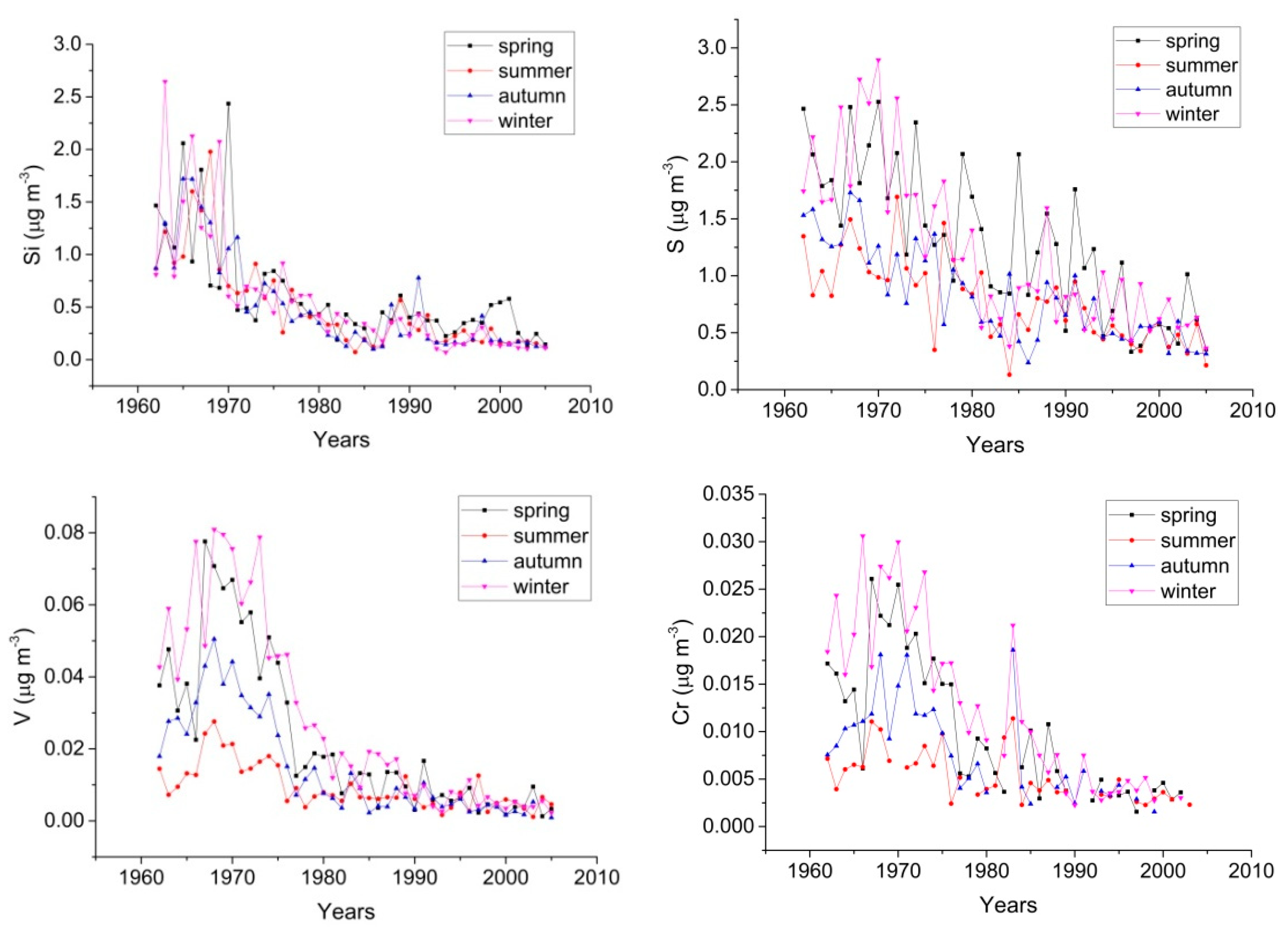
3.2. Seasonal Variation

Fluctuations in atmospheric concentrations of different chemical elements found in the air occur due to the varying weather conditions across seasons and the sources and emissions of air pollutants. The seasonality can cause significant changes in elemental concentrations in the study region. The mean seasonal concentrations for specific elements (Si, S, V, Cr, Ni, and Pb) are plotted as a function of time in Figure 4 (The rest of the elements are presented in Figure S2 in the Supplementary Materials).
Most of the studied elements present higher concentrations during the spring and winter periods. For example, the elements Fe, Si, K, Ca, Cu, V, Ni, S, Cr, Cl, and Al have higher concentrations during the cold months, rather than in summer and autumn. In winter, the emissions from energy production are at their seasonal maximum. From November to April, studded car tires knocked out particles from the asphalt of the street surface. In spring, the amount of precipitation is at its seasonal minimum. Therefore, airborne particles are not washed down moreefficiently than during the other seasons. Also, the sand spreads to the streets to increase friction during the winter and is easily resuspended into the air by vehicles passing by and by the wind. Simultaneously, in winter, the lower troposphere becomes stratified in the absence of solar heating, causing convective air flows. Thus, emitted air pollutants stay close to the ground and are not diluted upwards in the atmosphere [71].
Some elements present intense fluctuations in their concentrations like Cu (See Supplementary Materials, Figure S2. Its variations can be easily identified in the diagram concerning all seasons. The autumn period is more suitable for studying Cu, as these fluctuations are not so deep. No classification of Zn concentrations can be made depending on the season, as maxima and minima are presented in both warm and cold months. In the first two decades, fluctuations in Pb concentrations are intense, with the highest values occurring mainly in the winter and autumn seasons. After the 1980s, stabilization in Pb concentrations was observed.
Unfortunately, for some elements, there is a lack in the existing database. For example, there is a sharp fluctuation in Br concentrations during the first 20 years. After the 1980s, lower concentrations were observed during winter, while spring and summer had gained higher values of Br by that time. The cold season favors the emission of Cr in higher values than in the summer period. Na and Cl appear to follow the same behavior as Br and Cr, as the greatest variation in the specific elemental concentrations occurs during the winter months. Although data onAl concentrations are limited, reaching up to the middle of the 1980s, some conclusions about seasonal variation can be extracted, with spring and winter being the winners in higher elemental concentrations. Finally, Mn concentrations are mostly influenced during the autumn season.
The high concentrations of Cr, Mn, Pb, V, Fe, Al, Si, and Zn during the warm season, are explained by their tight connection with the soil-derived dust. Higher resuspended dust particles are favored by the dry conditions during the warm season. Furthermore, the more efficient vertical transport within the troposphere during the warm summer months results in lower concentrations of elements associated with “Pb(traffic)”, “Oil”, and “Traffic” during warm months. Also, between May and September, there is no need to heat buildings.

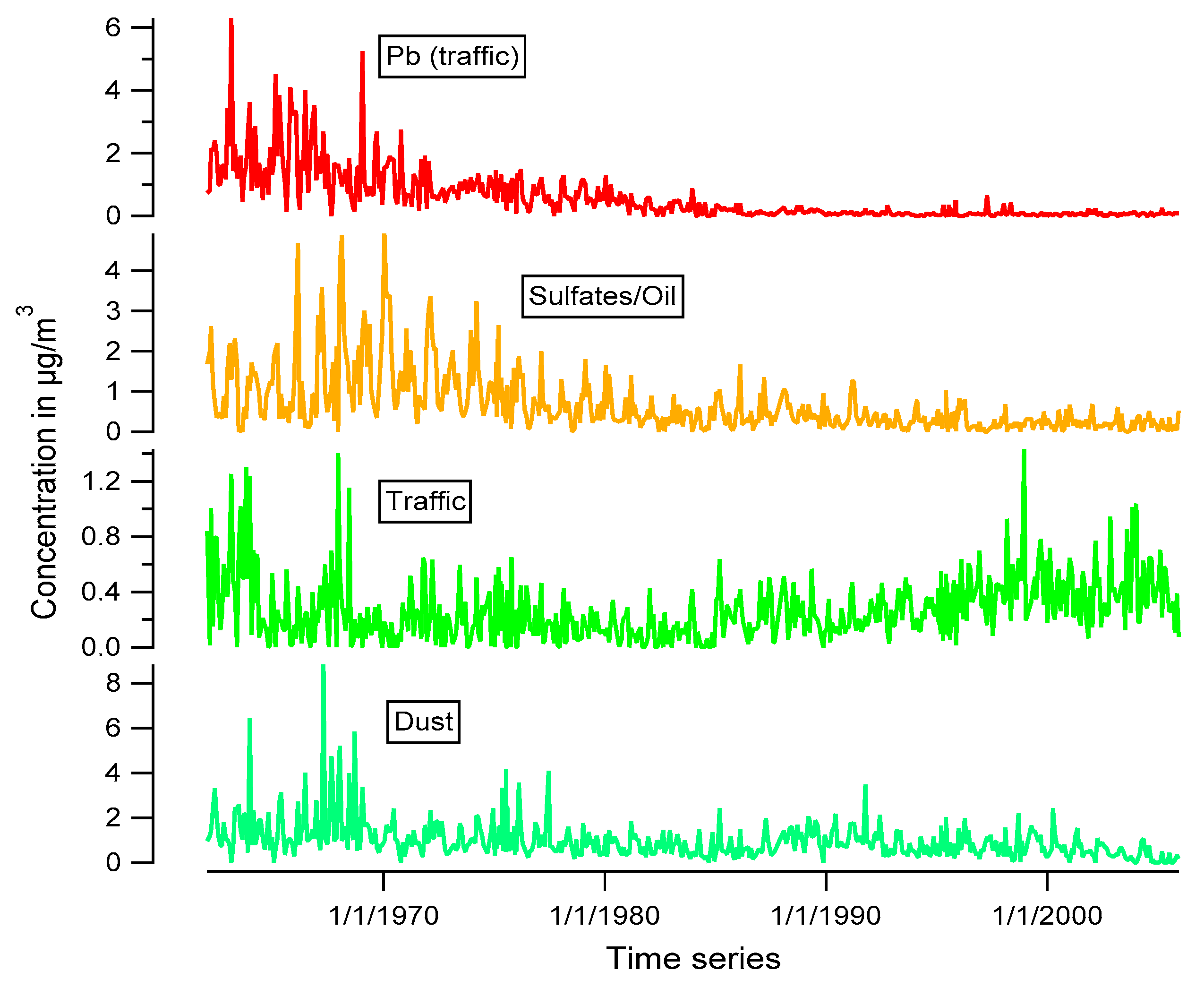
3.3. Source Apportionment

By using the source apportionment approach described in Section 2.2, we were able to identify four PM sources, each one defined by a corresponding factor (Figure 5). Since only elemental tracers were available and the resolution of the samples was very low, it was not possible to identify more PM sources.
The first factor (“Pb (traffic)”) explains the highest variation of Pb, Cl, and Si. Based on the time series of the factor, its emissions were higher before the mid-1970s and went to very low concentrations in the mid-1980s onwards (Figure 5 and Figure 6). This time trend follows the use of leaded fuel that started to face out in 1975 and was completely banned starting at the beginning of the 1990s until the end of the decade in all European countries. Because of concerns over air and soil lead levels and the accumulative neurotoxicity of lead, this leaded fuel has been designated as a Substance of Very High Concern in the European Union. It has been included in the Candidate List for Authorization under the REACH regulation, which involves the Registration, Evaluation, Authorization, and Restriction of Chemicals [72]. Japan became the first country to impose a total ban on leaded gasoline in 1986. From January 1993 onwards, all gasoline-fueled vehicles sold in the European Union were mandated to use unleaded fuel. Finland followed suit with its ban on leaded fuel in 1994 [73]. Pb was added to the fuel as tetraethyl lead (PbEt4) and was used until the 1990s as an additive in gasoline to prevent the engine from prematureignition (‘’knocking’’). Leaded gasoline has been banned within the EU from 2000 on, following Directive 98/70/EC and its amendment (Directive 2003/17/EC) [43]. When PbEt4 burns, it forms not only carbon dioxide and water but also lead, which can oxidize further to form compounds such as lead(II) oxide.
(CH3CH2)4Pb + 13O2 > 8CO2 + 10H20 + Pb
2Pb + O2 > 2PbO
Pb and PbO could accumulate and destroy the vehicle’s engine. To avoid that effect, lead scavengers 1,2-dibromoethane and 1,2-dichloroethane were used together with PbEt4. These additives form volatile lead(II) bromine and lead(II) chloride, respectively, which are flushed from the engine and into the air [74]. The latter can explain the high presence of Cl in this factor (“Pb (traffic)”).
The factor also explains to a smaller degree the variation of Si, Na, Cu, and Zn. All of these elements are well-known tracers of road dust [75], and their presence in the factor is justified. This factor might also affected by road-salting which could explain the presence of Na. Many calcium chloride, but also some chemicals like sodium and magnesium chloride, urea, sodium formate, and potassium acetate, areused in winter as a deicing agent. Their use depends highly on the severity of winter conditions.
The second factor (“Sulfates/Oil”) is traced by S, Ni, V, and Cr (Table 3: correlation coefficients: V-Ni (R2 = 0.93), V-Cr (R2 = 0.86), and V-S (R2 = 0.81)). As all of these elements are tracers of heavy oil combustion, this factor is identified as heavy oil combustion and secondary sulfates. Combustion of crude oil will produce particles containing V and Ni. Vanadium reacts with the oxygen from the combustion air forming V2O5 that creates layers on the heat exchangers and other boiler and stack surfaces. Additionally, V2O5 acts as a catalyst in the temperature range of 500–800 °C, accelerating the SO3 formation and greatly increasing its emissions [76]. In the absence of other tracers (e.g., EC), that could help separate a combustion process such as oil combustion to secondary formation of sulfates, it was impossible to separate the factor into two district sources. This factor hada higher contribution during the 1970s, most likely due to the higher use of oil during that time (Figure 6).
The third factor (“Traffic”) is a mixture of anthropogenic (Cu, Zn, Cr, Mn, and Br) and natural elements (Si, Na, K, Ti, and Fe) and it is identified as traffic-related resuspended dust (road dust) (Table 3 Si-K (R2 = 0.86), K-Na (R2 = 0.83)). In addition, the emissions from the exhaust of the vehicles and the emissions of PM precursors from the combustion of fuels and lubricants, vehicles emit substantial amounts of particles through the mechanical abrasion of brakes, clutch, tires, and motor [77]. These are deposited onto the road and re-suspended together with mineral dust particles and road wear minerals. Br and Cl in the factor might be an indication that the factor is slightly mixed with Pb-related traffic emissions. This is in a way expected as both factors represent traffic-related emissions. The factor had a higher contribution before the 1970s and the contribution increasedagain from the mid-1990s onwards (Figure 6). The first might be linked to increased emissions per car in that era (fuel quality might be an important factor here), while the latter with increasing car fleet number. At the end of 2005, there were about 2.8 million cars in traffic in Finland, of which about 2.4 were passenger cars. In 1962 (the beginning of the study time series), the number of car fleets was 344,703 (including passenger cars, vans, trucks, and buses) [78].
The final factor (“Dust”) is mostly composed of elements that are major components of soil (Al, Si, Na, S, K, Ca, Mn, and Fe) (Table 3: Ca-Si R2=0.90) and is identified as natural dust [79]. The source shows elevated contribution before the 1970s. This may be related to sand that was, and is still, dispersed on streets covered with snow in order to improve traffic safety by increasing the friction between the street surface and car tires and pedestrian shoes. In the old days the resulting ‘’street dust’’ was not considered to be a problem, but later enhanced street cleaning methods were adapted to solve the issue. Especially in the 1960s, an additional factor might have been emissions from construction activities. The surroundings of the sampling sites were still largely small wooden houses that were, in the name of progress, eagerly demolished and replaced by concrete buildings (Figure 6).

4. Conclusions

Forty-four years of weekly air filters from the city of Helsinki were analyzed for elemental concentrations of Na, Al, Si, S, Cl, K, Ca, Ti, V, Cr, Mn, Fe, Ni, Cu, Zn, Br, and Pb by XRF technique.
A declining trend has been noticed in all elemental concentrations. Pb is the element with the most important reduction, indicating the severeness and the effectiveness of the different regulations and measurements that had been taken and applied by the European Union since the 1970s. The declining trend of all elements presents the following order Cl(−22%) < Br(−32%) < Cu(−37%) < Ni(−61%) < Zn(−72%) < Na(−74%) < Mn(−77%) < Fe(−77%) < Ti(−80%) < K(−82%) = S(−82%) = Cr(−82%) < Al(−86%) < Si(−88%) < Ca(−89%) = V(−89%) < Pb(−95%).
Seasonal variations have been observed, with the maximum concentrations of the most elements appearing during the winter and spring seasons. During winter, the higher emissions from energy production, the increased resuspended dust fromthe streets, the lower troposphere and the absence of convective air flows have as a result higher concentrations of studied elements. On the contrary, the increased vertical transport within the troposphere during the warm months and the absence of central heating result in lower concentrations of elements associated with fuel sources, heavy oil combustion, and road dust sources.
Source apportionment analysis by applying the SoFi software revealed four emission sources: road dust (“Pb (traffic)”), heavy oil combustion/secondary sulfates (“Sulfates/Oil”), traffic emissions (“Traffic”), and natural dust–soil (“Dust”). The (“Pb (traffic)”) factor explains the highest emissions of Pb, Cl, and Si before the mid-1970s and very low concentrations in the mid-1980s onwards, being an index of the complete leaded fuel ban starting at the beginning of the 1990s in all European countries. The (“Sulfates/Oil”) factor had a higher contribution during the 1970s, most likely due to the higher use of oil during that time.The “Traffic” factor was higher before the 1970s due to the worst fuel quality in that era and increased emissions, while its contribution increasedagain from the mid-1990s due to the increasing car fleet number. The “Dust” factor had elevated contribution before the 1970s, related to the sand that was dispersed on streets covered with snow in order to improve traffic safety but without the enhanced street cleaning methods adopted currently.
We cannot extend the observation series to the present day, as the sampling station was closed down. However, the air quality monitoring programs of the city authorities indicate that the air quality situation after 2005 has been further improving gradually. The particle emissions of the Helsinki metropolitan area have decreased byhalf from 2005 to 2021. During the same period, the particle mass concentration has decreased about 40% [80].
A lot of surveys have been conducted for the same period, either in the rest part of Finland or in the neighboring countries (Norway, Sweden, and Russia). In the majority of them, the elemental concentrations in aerosols followed the same declines asin the current investigation, showing similar trends over the year. Based on the severe impact of air pollution on human health and the environment, it is crucial to continuously record the levels of trace elements in the atmosphere both nationally and internationally, apply new regulations about their reduction, and strictly control their emission sources for a better future.

Supplementary Materials

The following supporting information can be downloaded at: https://www.mdpi.com/article/10.3390/atmos14091430/s1, Figure S1: The Annual average concentrations of 17 chemical elements (Na, Al, Si, S, Cl, K, Ca, Ti, V, Cr, Mn, Fe, Ni, Cu, Zn, Br, Pb), in μg m−3, at Helsinki station (FMI). In the right corner of each diagram is noted the percentage reduction of each element. Figure S2: Average values of seasonal concentrations of trace elements, in μg m−3, through the years.

Author Contributions

Conceptualization, J.P., L.P., A.I. and K.E.; Methodology, E.I. and J.P.; Software, S.P. and M.I.M.; Validation, E.I., C.B., S.P. and M.I.M.; Formal analysis, E.I.; Investigation, E.I., J.P., S.P. and M.I.M.; Data curation, E.I., S.P. and M.I.M.; Writing-original draft preparation, E.I., C.B. and M.I.M.; Writing-review and editing; All authors; Visualization, J.P., M.I.M. and E.I.; Supervision, A.I. All authors have read and agreed to the published version of the manuscript.

Funding

This research received no external funding.

Institutional Review Board Statement

Not applicable.

Informed Consent Statement

Not applicable.

Data Availability Statement

Data is contained within the Supplementary Material.

Acknowledgments

We acknowledge support of this work by the project CALIBRA/EYIE (MIS 5002799), implemented under Action ‘’Reinforcement of the Research and Innovation Infrastructures’’, funded by the Operational Programme ‘’Comparativeness, Entrepreneurship and Innovation’’ (NSRF 2014–2020) and co-financed by Greece and the European Union (European Regional Development Fund).

Conflicts of Interest

The authors declare no conflict of interest.

References

  1. Miller, A.J.; Raduma, D.M.; George, L.A.; Fry, J.L. Source apportionment of trace elements and black carbon in an urban industrial area (Portland, Oregon). Atmos. Pollut. Res. 2019, 10, 784–794. [Google Scholar] [CrossRef]
  2. WHO. WHO Global Air Quality Guidelines: Particulate Matter (PM2.5 and PM10), Ozone, Nitrogen Dioxide, Sulfur Dioxide and Carbon Monoxide: Executive Summary. 2021. Available online: https://www.who.int/publications/i/item/9789240034433 (accessed on 22 September 2021).
  3. Taghvaee, S.; Sowlat, M.H.; Diapouli, E.; Manousakas, M.I.; Vasilatou, V.; Eleftheriadis, K.; Sioutas, C. Source apportionment of the oxidative potential of fine ambient particulate matter (PM2.5) in Athens, Greece. Sci. Total Environ. 2019, 653, 1407–1416. [Google Scholar] [CrossRef]
  4. Kyllönen, K.; Vestemius, M.; Anttila, P.; Makkonen, U.; Aurela, M.; Wängberg, I.; Mastromonaco, M.N.; Hakola, H. Trends and source apportionment of atmospheric heavy metals at a subarctic site during 1996–2018. Atmos. Environ. 2020, 236, 117644. [Google Scholar] [CrossRef]
  5. Lieu, W.; Wei, J.; Cai, M.; Qian, Z.; Long, Z.; Wang, L.; Vaughn, M.G.; Aaron, H.E.; Tong, X.; Li, Y.; et al. Particulate matter pollution and asthma mortality in China: A nationwide time-stratified case cross-over study from 2015–2020. Chemosphere 2022, 308, 136316. [Google Scholar] [CrossRef]
  6. Liu, B.; Zhang, Y.; Talifu, D.; Ding, X.; Wang, X.; Abulizi, A.; Zhao, Q.; Zhang, X.; Zhang, R. In Vitro Bioaccessibility and Health Risk of Heavy Metals from PM2.5/PM10 in Arid Areas-Hotan City, China. Atmosphere 2023, 14, 1066. [Google Scholar] [CrossRef]
  7. Manousakas, M.; Diapouli, E.; Papaefthymiou, H.; Migliori, A.; Karydas, A.G.; Padilla-Alvarez, R.; Bogovac, M.; Kaiser, R.B.; Jaksic, M.; Bogdanovic-Radovic, I.; et al. Source apportionment by PMF on elemental concentrations obtained by PIXE analysis of PM10 samples collected at the vicinity of lignite power plants and mines in Megalopolis, Greece. Nucl. Instrum. Methods Phys. Res. B 2015, 349, 114–124. [Google Scholar] [CrossRef]
  8. Kim, K.H.; Kabir, E.; Kabir, S. A review on the human health impact of airborne particulate matter. Environ. Int. 2015, 74, 136–143. [Google Scholar] [CrossRef]
  9. Almeida, S.M.; Faria, T.; Martins, V.; Canha, N.; Diapouli, E.; Eleftheriadis, K.; Manousakas, M.I. Source apportionment of children daily exposure to particulate matter. SSRN Electron. J. 2022, 835, 155349. [Google Scholar] [CrossRef]
  10. Gu, X.Y.; Chu, X.; Zeng, X.L.; Bao, H.R.; Liu, X.J. Effects of PM2.5 exposure on the Notch signaling pathway and immune imbalance in chronic obstructive pulmonary disease. Environ. Pollut. 2017, 226, 163–173. [Google Scholar] [CrossRef]
  11. Buoli, M.; Grassi, S.; Caldiroli, A.; Carnevali, G.S.; Mucci, F.; Iodice, S.; Cantone, L.; Pergoli, L.; Bollati, V. Is there a link between air pollution and mental disorders? Environ. Int. 2018, 118, 154–168. [Google Scholar] [CrossRef]
  12. Lee, S.; Kang, J.E. Impact of particulate matter and urban spatial characteristics on urban vitality using spatiotemporal big data. Cities 2022, 131, 104030. [Google Scholar] [CrossRef]
  13. Zhang, C.; Hu, Y.; Adams, M.D.; Liu, M.; Li, B.; Shi, T.; Li, C. Natural and human factors influencing urban particulate matter concentrations in central heating areas with long-term wearable monitoring devices. Environ. Res. 2022, 215, 114393. [Google Scholar] [CrossRef] [PubMed]
  14. Seinfeld, J.H.; Pandis, S.N. Atmospheric Chemistry and Physics: From Air Pollution to Climate Change; Wiley: New York, NY, USA, 1998. [Google Scholar]
  15. Wagner, A.; Boman, J.; Gatari, M.J. Elemental analysis of size-fractionated particulate matter sampled in Göteborg, Sweden. Spectrochim. Acta Part B At. Spectrosc. 2008, 63, 1426–1431. [Google Scholar] [CrossRef]
  16. Boman, J.; Wagner, A.; Gatari, M.J. Trace elements in PM2.5 in Gothenburg, Sweden. Spectrochim. Acta Part B At. Spectroscopy 2010, 65, 478–482. [Google Scholar] [CrossRef]
  17. Pacyna, J.M.; Pacyna, E.G. An assessment of global and regional emissions of trace metals to the atmosphere from anthropogenic sources worldwide. Environ. Rev. 2001, 9, 269–298. [Google Scholar] [CrossRef]
  18. Christian, T.J.; Yokelson, R.J.; Cárdenas, B.; Molina, L.T.; Engling, G.; Hsu, S.C. Trace gas and particle emissions from domestic and industrial biofuel use and garbage burning in central Mexico. Atmos. Chem. Phys. 2010, 10, 565–584. [Google Scholar] [CrossRef]
  19. Dung, T.T.T.; Vassilieva, E.; Swennen, R.; Cappuyns, V. Release of Trace Elements from Bottom Ash from Hazardous Waste Incinerators. Recycling 2018, 3, 36. [Google Scholar] [CrossRef]
  20. EEA. Heavy Metal Emissions; European Environmental Agency: 2020. Available online: https://www.eea.europa.eu/data-and-maps/indicators/eea32-heavy-metal-hm-emissions-1/assessment-10 (accessed on 22 September 2021).
  21. Diapouli, E.; Manousakas, M.; Vratolis, S.; Vasilatou, V.; Maggos, T.; Saraga, D.; Grigoratos, T.; Argyropoulos, G.; Voutsa, D.; Samara, C.; et al. Evolution of air pollution source contributions over one decade, derived by PM10 and PM2.5 source apportionment in two metropolitan urban areas in Greece. Atmos. Environ. 2017, 164, 416–430. [Google Scholar] [CrossRef]
  22. AMAP. AMAP Assessment 2002: Heavy Metals in the Arctic; first published as electronic document in 2004; Arctic Monitoring and Assessment Programme (AMAP): Oslo, Norway, 2005; p. Xvi+265. ISBN 82-7971-018-3. [Google Scholar]
  23. Anttila, P.; Salmi, T. Characterizing temporal and spatial patterns of urban PM10 using six years of Finnish monitoring data. Boreal Environ. Res. 2006, 11, 463–479. [Google Scholar]
  24. Infante, R.; Acosta, I.L. Size distribution of trace metals in Ponce, Puerto Rico air particulate matter. Atmos. Environ. Part B Urban Atmos. 1991, 25, 121–131. [Google Scholar] [CrossRef]
  25. Pacyna, J.M.; Pacyna, E.G.; Aas, W. Changes of emissions and atmospheric deposition of mercury, lead and cadmium. Atmos. Environ. 2009, 43, 117–127. [Google Scholar] [CrossRef]
  26. EU. Council Directive 1999/30/EC of 22 April 1999 Relating to Limit Values for Sulfur Dioxide, Nitrogen Dioxide and Oxides of Nitrogen, Particulate Matter and Lead in Ambient Air. Off. J. 1999, L163, 41–60. Available online: http://eurlex.europa.eu/LexUriServ.do?uri=CELEX:31999L0030 (accessed on 22 September 2021).
  27. EU. Directive 2004/107/EC of the European Parliament and of the Council of 15 December 2004 Relating to Arsenic, Cadmium, Mercury, Nickel and Polycyclic Aromatic Hydrocarbons in Ambient Air. Off. J. 2004, L23, 3–16. Available online: http://eurlex.europa.eu/LexUriServ/LexUriServ.do?uri=OJ:L:2005:023:0003:0016 (accessed on 22 September 2021).
  28. EU. Directive 2008/50/EC of the European Parliament and of the Council of 21 May 2008 on Ambient air Quality and Cleaner Air for Europe. Off. J. 2008, L152, 1–44. Available online: http://eurlex.europa.eu/legal-content/EN/TXT/PDF/?uri=CELEX:32008L0050from=EN (accessed on 22 September 2021).
  29. EU. Commission Directive (EU) 2015/1480 of 28 August 2015 Amending Several Annexes to Directives 2004/107/EC and 2008/50/EC of the European Parliament and of the Council Laying Down the Rules Concerning Reference Methods, Data Validation and Location of Sampling Points for the Assessment of Ambient Air Quality. Off. J. 2015, L226, 4–11. Available online: https://eurlex.europa.eu/eli/dir/2015/1480/oj (accessed on 22 September 2021).
  30. Wiklund, J.A.; Kirk, J.L.; Muir, D.C.G.; Gleason, A.; Carrier, J.; Yang, F. Atmospheric trace metal deposition to remote Northwest Ontario, Canada: Anthropogenic fluxes and inventories from 1860 to 2010. Sci. Total Environ. 2020, 749, 142276. [Google Scholar] [CrossRef]
  31. Kyllönen, K.; Karlsson, V.; Ruoho-Airola, T. Trace elements deposition and trends during a ten year period in Finland. Sci. Total Environ. 2009, 407, 2260–2269. [Google Scholar] [CrossRef] [PubMed]
  32. Laing, J.R.; Hopke, P.K.; Kopke, E.F.; Husian, L.; Dutkiewicz, V.A.; Paatero, J.; Viisanen, Y. Long-term particle measurements in Finnish Arctic: Part I—Chemical composition and trace metal solubility. Atmos. Environ. 2014, 88, 275–284. [Google Scholar] [CrossRef]
  33. Laing, J.R.; Hopke, P.K.; Hopke, E.F.; Husian, L.; Dutkiewicz, V.A.; Paatero, J.; Viisanen, Y. Long-term particle measurements in Finnish Arctic: Part II—Trend analysis and source location identification. Atmos. Environ. 2014, 88, 285–296. [Google Scholar] [CrossRef]
  34. Jalkanen, L.; Mäkinen, A.; Häsänen, E.; Juhanoja, J. The effect of large anthropogenic particulate emissions on atmospheric aerosols, deposition and bioindicators in the eastern Gulf of Finland region. Sci. Total Environ. 2000, 262, 123–126. [Google Scholar] [CrossRef]
  35. Hosiokangas, J.; Ruuskanen, J.; Pekkanen, J. Effects of soil dust episodes and mixed fuel source on source apportionment of PM10 particles in Kuopio, Finland. Atmos. Environ. 1999, 33, 3821–3829. [Google Scholar] [CrossRef]
  36. Vallius, M.; Ruuskanen, J.; Mirme, A.; Pekkanen, J. Concentrations and estimated soot content of PM1, PM2.5 and PM10 in subarctic urban atmosphere. Environ. Sci. Technol. 2000, 34, 1919–1925. [Google Scholar] [CrossRef]
  37. Pakkanen, T.; Loukkola, K.; Korhonen, C.; Aurela, M.; Mäkelä, T.; Hillamo, R.; Aamio, P.; Koskentalo, T.; Kousa, A.; Maenhaut, W. Sources and chemical composition of atmospheric fine and coarse particles in the Helsinki area. Atmos. Environ. 2001, 35, 5381–5391. [Google Scholar] [CrossRef]
  38. Pohjola, M.; Kousa, A.; Kukkonen, J.; Härkönen, J.; Karppinen, A.; Aamio, P.; Koskentalo, T. The spatial and temporal variation of measured urban PM10 and PM2.5 in the Helsinki metropolitan area. Urban Air Qual.-Recent Advances. 2002, 2, 189–201. [Google Scholar] [CrossRef]
  39. Laakso, L.; Hussein, T.; Aamio, P.; Komppula, M.; Hiltunen, V.; Viisanen, Y.; Kulmala, M. Diurnal and annual characteristics of particle mass and number concentrations in urban, rural and arctic environments in Finland. Atmos. Environ. 2003, 37, 2629–2641. [Google Scholar] [CrossRef]
  40. Hosiokangas, J.; Vallius, M.; Ruuskanen, J.; Mirme, A.; Pekkanen, J. Resuspended dust episodes as an urban air-quality problem in subarctic regions. Scand. J. Work. Environ. Health 2004, 30, 28–35. [Google Scholar] [PubMed]
  41. Kukkonen, J.; Pohjola, M.; Sokhi, R.S.; Luhana, L.; Kitwiroon, N.; Fragkou, L.; Rantamäki, M.; Berge, E.; Ødegaard, V.; Slørdal, L.H.; et al. Analysis and evaluation of selected local-scale PM10 air pollution episodes in four European cities: Helsinki, London, Milan and Oslo. Atmos. Environ. 2005, 39, 2759–2773. [Google Scholar] [CrossRef]
  42. Berg, T.; Aas, W.; Pacyna, J.; Uggerud, H.; Vdste, M. Atmospheric trace metal concentrations at Norwegian background sites during 25 years and its relation to European emissions. Atmos. Environ. 2008, 42, 7494–7501. [Google Scholar] [CrossRef]
  43. Kummer, U.; Pacyna, J.; Pacyna, E.; Friedrich, R. Assessment of heavy metal releases from the use phase of road transport in Europe. Atmos. Environ. 2009, 43, 640–647. [Google Scholar] [CrossRef]
  44. Pacyna, J.M.; Pacyna, E.G.; Panasiuk, D.; Fudala, J.; Strzelecka-Jastrzab, E.; Hlawiczka, S. Heavy metals emissions in Europe: First results from the EU ESPREME project. In Proceedings of the Joint Workshop of the UN ECE Task Force on Emission Inventories and Projections at the EU ESPREME Project, Rovaniemi, Finland, 18–19 October 2005. [Google Scholar]
  45. Victorin, K. Health effects of urban air pollutants. Guideline values and conditions in Sweden. Chemosphere 1993, 27, 1691–1706. [Google Scholar] [CrossRef]
  46. Mukai, H.; Machida, T.; Tanaka, A.; Vera, Y.P.; Uematsu, M. Lead isotope ratios in the urban air of eastern and central Russia. Atmos. Environ. 2001, 35, 2783–2793. [Google Scholar] [CrossRef]
  47. Shevchenko, V.; Lisitzin, A.; Vinogradova, A.; Stein, R. Heavy metals in aerosols over the seas of the Russian Arctic. Sci. Total Environ. 2003, 306, 11–25. [Google Scholar] [CrossRef]
  48. Voukantsis, D.; Karatzas, K.; Kukkonen, J.; Räsänen, T.; Karppinen, A.; Kolehmainen, M. Intercomparison of air quality data using principal component analysis, and forecasting of PM10 and PM2.5 concentrations using artificial neural networks, in Thessaloniki and Helsinki. Sci. Total Environ. 2011, 409, 1266–1276. [Google Scholar] [CrossRef]
  49. Mattsson, R.; Jaakkola, T. An Analysis of Helsinki Air 1962 to 1977 Based on Trace Metals and Radionuclides. Geophysica 1979, 16, 1–42. [Google Scholar]
  50. Paatero, J.; Hatakka, J.; Mattsson, R.; Lehtinen, I. A Comprehensive Station for Monitoring Atmospheric Radioactivity. Radiat. Prot. Dosim. 1994, 54, 33–39. [Google Scholar] [CrossRef]
  51. Mattsson, R.; Paatero, J.; Hatakka, J. Automatic Alpha/Beta Analyser for Air Filter Samples-Absolute Determination of Radon Progeny by Pseudo-coincidence Techniques. Radiat. Prot. Dosim. 1996, 63, 133–139. [Google Scholar] [CrossRef]
  52. Manousakas, M.; Diapouli, E.; Papaefthymiou, H.; Kentarelou, V.; Zarkadas, C.; Kalogridis, A.C.; Karydas, A.C.; Eleftheriadis, K. XRF characterization and source apportionment of PM10 samples collected in a coastal city. X-ray Spectrom. 2017, 47, 190–200. [Google Scholar] [CrossRef]
  53. Canonaco, F.; Crippa, M.; Slowik, J.G.; Baltensperger, U.; Prévôt, A.S.H. SoFi, an IGOR-based interface for the efficient use of the generalized multilinear engine (ME-2) for the source apportionment: ME-2 application to aerosol mass spectrometer data. Atmos. Meas. Tech. 2013, 6, 3649–3661. [Google Scholar] [CrossRef]
  54. Belis, C.A.; Karagulian, F.; Larsen, B.R.; Hopke, P.K. Critical review and meta-analysis of ambient particulate matter source apportionment using receptor models in Europe. Atmos. Environ. 2013, 69, 94–108. [Google Scholar] [CrossRef]
  55. Polissar, A.V.; Hopke, P.K.; Poirot, R.L. Atmospheric aerosol over Vermont: Chemical composition and sources. Environ. Sci. Technol. 2001, 35, 4604–4621. [Google Scholar] [CrossRef] [PubMed]
  56. Reff, A.; Eberly, S.I.; Bhave, P.V. Receptor Modeling of Ambient Particulate Matter Data Using Positive Matrix Factorization: Review of Existing Methods. J. Air Waste Manag. Assoc. 2007, 57, 146–154. [Google Scholar] [CrossRef] [PubMed]
  57. Canonaco, F.; Tobler, A.; Chen, G.; Sosedova, Y.; Slowik, J.G.; Bozzetti, C.; Daellenbach, K.R.; El Haddad, I.; Crippa, M.; Huang, R.J.; et al. A new method for long-term source apportionment with time-dependent factor profiles and uncertainty assessment using SoFi Pro: Application to 1 year of organic aerosol data. Atmos. Meas. Tech. 2021, 14, 923–943. [Google Scholar] [CrossRef]
  58. Kotz, S.; Johnson, N.L.; Read, C.B. Encyclopedia of Statistical Sciences, 1st ed.; Wiley: New York, NY, USA, 2006; Volume 9. [Google Scholar]
  59. Nriagu, J.O. A global assessment of natural sources of atmospheric trace metals. Nature 1989, 338, 47–49. [Google Scholar] [CrossRef]
  60. Athanasopoulou, E.; Tombrou, M.; Russell, A.G.; Karanasiou, A.; Eleftheriadis, K.; Dandou, A. Implementation of road and soil dust emission parameterizations in the aerosol model CAMx: Applications over the greater Athens urban area affected by natural sources. J. Geophys. Res. 2010, 115, D17301. [Google Scholar] [CrossRef]
  61. Chapman, S. Notes of Atmospheric Sodium. Astrophys. J. 1939, 90, 309. [Google Scholar] [CrossRef]
  62. Zhuang, H.; Chan, C.K.; Fang, M.; Wexler, A.S. Formation of nitrate and non-sea-salt sulfate on coarse particles. Atmos. Environ. 1999, 33, 4223–4233. [Google Scholar] [CrossRef]
  63. Eleftheriadis, K.; Ochsenkuhn, K.M.; Lymperopoulou, T.; Karanasiou, A.; Razos, P.; Ochsenkuhn-Petropoulou, M. Influence of local and regional sources on the observed spatial and temporal variability of size resolved atmospheric aerosol mass concentrations and water-soluble species in the Athens metropolitan area. Atmos. Environ. 2014, 97, 252–261. [Google Scholar] [CrossRef]
  64. Lucarelli, F.; Mandò, P.A.; Nava, S.; Prati, P.; Zucchiatti, A. One-year study of the elemental composition and source apportionment of PM10 aerosols in Florence, Italy. J. Air Waste Manag. Assoc. 2014, 54, 1372–1382. [Google Scholar] [CrossRef]
  65. Viana, M.; Kuhlbusch, T.A.J.; Querol, X.; Alastuey, A.; Harrison, R.M.; Hopke, P.K.; Winiwarter, W.; Vallius, M.; Szidat, S.; Prevôt, A.S.H.; et al. Source apportionment of particulate matter in Europe: A review of methods and results. J. Aerosol Sci. 2008, 39, 827–849. [Google Scholar] [CrossRef]
  66. Santoso, M.; Hopke, P.K.; Hidayat, A.; Dwiana, D.L. Sources identification of the atmospheric aerosol at urban and suburban sites in Indonesia by positive matrix factorization. Sci. Total Environ. 2008, 397, 229–237. [Google Scholar] [CrossRef]
  67. Pacyna, J. Workpackage 02-D01b Source-Sector Analysis and Evaluation Report. Estimation of Willingness-to-Pay to Reduce Risks of Exposure to Heavy Metals and Cost-Benefit Analysis for Reducing Heavy Metals Occurrence in Europe. 2007. Available online: http://espreme.ier.uni-stuttgart.de/ (accessed on 22 September 2021).
  68. EEA. European Union Emission Inventory Report 1990-2017 under the UNECE Convection on Long-Range Transboundary Air Pollution (LRTAP), EEA Report No 08/2019. 2019; ISBN 978-92-9480-078-7.
  69. Virkkula, A.; Teinilä, K.; Hillamo, R.; Stohl, A. A decade of trace gas measurements using DOAS in Finnish Lapland. Boreal Environ. Res. 2003, 8, 351–363. [Google Scholar]
  70. Jokiniemi, J.; Raunemaa, T.; Mattsson, R.; Hautojärvi, A. Analysis of aerosol samples from radioactivity registration stations. Nucl. Instrum. Methods Phys. Res. Sect. B Beam Interact. Mater. At. 1984, 3, 451–453. [Google Scholar] [CrossRef]
  71. Li, Z.; Guo, J.; Ding, A.; Liao, H.; Liu, J.; Sun, Y.; Wang, T.; Xue, H.; Zhang, H.; Zhu, B. Aerosol and boundary-layer interactions and impact on air quality. Natl. Sci. Rev. 2017, 4, 810–833. [Google Scholar] [CrossRef]
  72. ECHA. Inclusion of Substances of Very High Concern in the Candidate List—Decision of the European Chemicals Agency ED/169/2012. 2012. Available online: https://echa.europa.eu/documents/10.162/0b417b76-b533-42a1-9bd2-519fldc1990d (accessed on 22 September 2021).
  73. NESTE. Bensiiniopas, Neste Oyj; Engineering Services Company: Espoo, Finland, 2022. [Google Scholar]
  74. Kloprogge, J.T.; Ponce, C.P.; Loomis, T.A. The Periodic Table: Nature’s Building Blocks; Kloprogge, J.T., Ponce, C.P., Loomis, T.A., Eds.; Elsevier: Amsterdam, The Netherlands, 2021. [Google Scholar]
  75. Manousakas, M.; Diapouli, E.; Belis, C.A.; Vasilatou, V.; Gini, M.; Lucarelli, F.; Querol, X.; Eleftheriadis, K. Quantitative Assessment of the variability in chemical profiles from source apportionment analysis of PM10 and PM2.5 at different sites within a large Metropolitan area. Environ. Res. 2021, 192, 110257. [Google Scholar] [CrossRef]
  76. Kim, E.; Hopke, P.K. Source characterization of ambient fine particles at multiple sites in the Seattle area. Atmos. Environ. 2008, 42, 6047–6056. [Google Scholar] [CrossRef]
  77. Lopes, D.; Rafael, S.; Ferreira, J.; Relvas, H.; Almeida, S.M.; Faria, T.; Martins, V.; Diapouli, E.; Manousakas, M.; Vasilatou, V.; et al. Assessing the levels of regulated metals in an urban area: A modeling and experimental approach. Atmos. Environ. 2022, 290, 119366. [Google Scholar] [CrossRef]
  78. Traficom. Open Data for Vehicles; The Finnish Transport and Communications Agency Traficom: Helsinki, Finland, 2022. [Google Scholar]
  79. Gini, M.; Manousakas, M.I.; Karydas, A.G.; Eleftheriadis, K. Mass size distributions composition and dose estimates of particulate matter in Saharan dust outbreaks. Environ. Pollut. 2022, 298, 118768. [Google Scholar] [CrossRef]
  80. Korhonen, S.; Loukkola, K.; Portin, H.; Niemi, J. Ilmanlaatu Pääkaupunkiseudullavuonnav2021—Vuosiraportti; HSY:n julkaisuja 3/2022; Helsingin seudunympäristöpalvelut -kuntayhtymä: Helsinki, Finland, 2022. [Google Scholar]
Figure 1. Location of the measurement sites, Finnish Meteorological Institute, in Helsinki. Blue circle: 1962–1966 (60°11′ N, 24°57′ E), red circle: 1967–2005 (60°10′ N, 24°57′ E) (aerial photo: National Land Survey of Finland, CC BY 4.0).
Atmosphere 14 01430 g001
Figure 2. The annual average concentrations of Si, S, V, Cr, Ni, Pb elements (in μg m−3) at Helsinki station (FMI). In the right corner of each diagram, the percentage reduction of each element is noted.
Atmosphere 14 01430 g002
Figure 3. Total percentage decrease in elemental concentrations.
Atmosphere 14 01430 g003
Figure 4. Mean values of seasonal concentrations of trace elements, in μg m-3, through the years.
Atmosphere 14 01430 g004aAtmosphere 14 01430 g004b
Figure 5. Source profiles. The bars represent the normalized concentrations of the tracers to the factors, while the stars represent the normalized contribution of the factor to the element. Different colours represent different sources.
Atmosphere 14 01430 g005
Figure 6. Time series of source contributions. The contribution does not refer to PM mass but to the sum of the species (elements) used as tracers in the source apportionment analysis.
Atmosphere 14 01430 g006
Table 1. The expanded measurement uncertainties (MU) and calculated limits of detections (LOD) in μg m−3 of elements measured by the ED-XRF spectrometer.
Element(MU)
(%)
Number of
Samples
LOD
(μg m−3)
Na30.25990.0307
Al16.05990.0098
Si15.85990.0028
S9.15990.0009
Cl15.85990.0009
K9.15990.0009
Ca10.45990.0068
Ti10.95990.0025
V13.25990.0015
Cr21.25990.0025
Mn16.85990.0012
Fe10.45990.0012
Ni17.85990.0009
Cu11.25990.0012
Zn12.15990.0015
Br18.05990.0012
Pb13.55990.0022
Table 2. The multiannual minimum, maximum, median, mean concentrations, standard deviation (in μg m−3), skewness, kurtosis, and total percentage decrease in elemental concentrations, for the studied period (1962–2005), obtained from the FMI station.
ElementMinMaxMedianMeanSt. Dev.SkewnessKurtosisTotal Decrease
(μg m−3) (%)
Na0.071.370.260.300.192.126.79−74.0
Al<0.011.040.090.130.132.8811.79−86.0
Si0.033.840.380.550.582.9611.17−88.0
S0.095.120.841.020.711.533.31−82.0
Cl<0.010.490.020.030.066.0346.16−22.0
K<0.011.210.170.220.152.227.82−82.0
Ca0.011.760.170.210.193.4017.65−89.0
Ti<0.010.150.010.020.014.0827.08−80.0
V<0.010.140.010.020.021.884.10−89.0
Cr<0.010.050.010.010.011.704.07−82.0
Mn<0.010.180.010.010.016.5463.16−77.0
Fe0.011.560.180.210.153.6023.58−77.0
Ni<0.010.040.000.010.011.974.55−61.0
Cu<0.010.440.020.030.045.3640.71−37.0
Zn<0.010.440.040.060.052.6510.08−72.0
Br<0.010.110.010.010.023.8116.60−32.0
Pb<0.011.960.100.170.233.6719.91−95.0
Table 3. Correlation coefficients between the 17 elements.
NaAlSiSClKCaTiVCrMnFeNiCuZnBrPb
Na1
Al0.871
Si0.890.861
S0.810.830.841
Cl−0.24−0.32−0.21−0.301
K0.910.810.930.85−0.131
Ca0.850.830.900.79−0.180.921
Ti0.880.890.810.82−0.210.860.841
V0.800.830.830.90−0.310.780.690.801
Cr0.760.720.760.83−0.340.680.590.670.931
Mn0.340.610.450.31−0.130.420.440.440.260.181
Fe0.870.890.880.81−0.150.890.940.910.770.670.421
Ni0.820.830.820.87−0.280.780.700.830.960.870.260.791
Cu0.510.430.380.29−0.110.430.400.480.340.400.080.500.381
Zn0.860.700.840.68−0.120.890.810.760.660.600.290.810.720.621
Br0.500.540.330.43−0.020.360.350.400.420.320.190.400.400.210.221
Pb0.810.770.960.84−0.260.870.780.690.860.820.370.750.820.280.770.291
Disclaimer/Publisher’s Note: The statements, opinions and data contained in all publications are solely those of the individual author(s) and contributor(s) and not of MDPI and/or the editor(s). MDPI and/or the editor(s) disclaim responsibility for any injury to people or property resulting from any ideas, methods, instructions or products referred to in the content.

