Assessment of the Influence of Instrument Parameters on the Detection Accuracy of Greenhouse-Gases Absorption Spectrometer-2 (GAS-2)

Abstract

Satellite-based monitoring of atmospheric greenhouse gas (GHG) concentrations has emerged as a prominent and globally recognized field of research. With the imminent launch of the Greenhouse-Gases Absorption Spectrometer-2 (GAS-2) on the FengYun3-H (FY3-H) satellite in 2024, there is a promising prospect for substantial advancements in GHG detection capabilities. Crucially, the accurate acquisition of spectral information by GAS-2 is heavily reliant on its instrument parameters. However, the existing body of research predominantly emphasizes the examination of atmospheric parameters and their impact on GHG detection accuracy, thereby leaving a discernible gap in the comprehensive evaluation of instrument parameters specifically concerning the acquisition of atmospheric greenhouse gas concentration data by GAS-2. To address this knowledge gap, our study employs a radiation transfer model grounded in radiation transfer theory. This comprehensive investigation aims to quantitatively analyze the effects of various instrument parameters, encompassing crucial aspects such as spectral resolution, spectral sampling rate, signal-to-noise ratio, radiometric resolution, and spectral calibration accuracy (including instrument line shape function, central wavelength shift, and spectral resolution broadening). Based on our preliminary findings, it is evident that GAS-2 has the necessary spectral resolution, spectral sampling rate, and signal-to-noise ratio, slightly surpassing existing international instruments and enabling a significant detection accuracy level of 1 part per million (ppm). Moreover, it is essential to recognize the critical impact of instrument spectral calibration accuracy on overall detection precision. Among the five commonly used instrument line shape functions, the sinc function has the least impact on detection accuracy. Additionally, GAS-2’s radiance quantization depth is 14 bits, which is comparable to similar international payloads and maintains a root mean squared error below 0.1 ppm, thus ensuring a high level of precision. This study provides a comprehensive evaluation of the influence of GAS-2’s instrument parameters on detection accuracy, offering valuable insights for the future development of spectral calibration, the optimization of similar payload instrument parameters, and the overall improvement of instrument quantification capabilities.

1. Introduction

The continuing growth of the global economy and society has resulted in an alarming increase in the concentration of greenhouse gases (GHGs) in the Earth’s atmosphere [1]. According to the World Meteorological Organization, the concentration of carbon dioxide (CO${}_2$) had reached 413.2 parts per million (ppm) by 2020 [2], while methane (CH${}_4$) had reached 1889 parts per billion (ppb). This escalating trend amplifies the likelihood of climate extremes, such as soaring temperatures, intense precipitation, melting ice caps, rising sea levels, and acidification of the oceans, thereby imposing profound economic and societal consequences [3]. Considering that human activities are the primary sources of GHGs, it is essential to comprehend their impact on the fluctuation of atmospheric carbon dioxide and methane concentrations. This understanding assumes paramount significance in the face of climate change. Currently, terrestrial monitoring networks constitute the primary means of obtaining atmospheric CO${}_2$ concentrations [4]. However, this approach suffers from inherent limitations, such as high costs and limited spatial coverage, especially in vast polar regions, deserts, mountains, and other remote areas. Consequently, the scarcity of data severely restricts the practical application of observation results derived from these networks. To overcome these challenges, the utilization of satellite platforms for atmospheric CO${}_2$ observation has emerged as a pivotal solution [5]. Satellite-based observation not only offers a cost-effective alternative but also provides extensive spatial coverage, including previously inaccessible regions. This has significantly enhanced our capacity to monitor and analyze atmospheric CO${}_2$ concentrations on a global scale [6].

Satellite sensors used for greenhouse gas (GHG) monitoring are currently classified into two categories: passive detection and active detection, based on their working modes [7]. Passive detection involves remote sensing instruments that do not emit electromagnetic waves toward the target being observed. Instead, they directly receive and record either the reflected or scattered solar spectrum from the target or the emitted electromagnetic waves emitted by themselves. The passive detection methods encompass grating spectroscopy, interference spectroscopy, and spatial heterodyne spectroscopy. In the early stages of GHG detection, grating spectroscopic payloads such as SCIAMACHY and AIRS were employed [8,9]. Interferometric payloads, e.g., IMG, ACE-FTS, IASI, and CrIS were also utilized [10]. More recently, dedicated GHG payloads based on Michelson interference spectroscopy technology, such as TANSO-FTS, TANSO-FTS2 mounted on GOSAT, and FengYun-3D GAS (Greenhouse gases Absorption Spectrometer), have been developed [11,12,13]. Furthermore, payloads such as OCO-2 (Orbiting Carbon Observatory-2), OCO-3, and TanSat utilize grating splitting technology [14,15,16]. Notably, Gaofen-5’s GMI payload, launched in 2018 [17], stands as the world’s pioneering greenhouse gas monitor utilizing spatial heterodyne spectroscopy technology. The second category, active detection, involves remote sensing instruments that actively emit electromagnetic waves of specific wavelengths toward the target. The remote sensor then receives and records the electromagnetic waves reflected from the target, enabling the retrieval of concentration information regarding the target gas based on its distinctive characteristics. DQ-1, launched in 2022 [18], represents the world’s first active greenhouse gas remote-sensing satellite currently deployed in polar orbit. Additionally, there are planned active detection payloads under development, such as ASCENDS and A-SCOPE [19,20].

Accurately detecting global atmospheric greenhouse gases using satellite platforms presents a formidable challenge due to the high precision required for measurements. The annual change in greenhouse gas concentration in the atmosphere is approximately 1.5 ppm [21], indicating a relatively small concentration change. Achieving high detection accuracy is crucial to generate reliable and applicable results. Extensive satellite remote sensing experiments have unveiled that accurate data retrieval is influenced by three primary factors: instrument performance, atmospheric parameters, and surface characteristics [22,23]. To mitigate systematic errors stemming from these factors, precise calibration and correction methods are indispensable. It is imperative to carefully assess and account for these factors to ensure the reliability and accuracy of retrieval results. Thus, a comprehensive assessment and calibration of these factors play a pivotal role in obtaining accurate atmospheric measurements through remote sensing. By effectively considering and accounting for these factors, we can significantly enhance the accuracy of atmospheric detection and contribute to a deeper understanding of the intricate processes governing atmospheric phenomena.

Zhang Xingying et al. analyzed the main factors influencing the accuracy of greenhouse gas retrieval, including (1) the detection accuracy of remote sensors; (2) the accuracy of the greenhouse gas retrieval algorithm; (3) atmospheric clouds and aerosols; and (4) the accuracy of benchmark validation data from the ground-based site [24]. Li Qinqin et al. investigated the impact of surface pressure, atmospheric temperature profile, surface albedo, aerosol optical thickness, and other factors on carbon dioxide retrieval, while analyzing the error of the spatial heterodyne spectrometer GMI [25]. Jun Wu et al. and Hanhan Ye et al. explored and analyzed the influence of spectral resolution, altitude, surface albedo, and initial carbon dioxide concentration on the detection accuracy of greenhouse gases [26,27]. Yoshida et al. and Uchino et al. identified several factors contributing to systematic errors in the retrieval of atmospheric carbon dioxide (CO${}_2$) and methane (CH${}_4$) concentrations using GOSAT data [28,29]. These factors encompass aerosol optical depth (AOD) and surface pressure, both of which result in significant errors in the retrieval results. Similarly, Connor et al. investigated the influence of environmental factors such as AOD, surface pressure, and temperature on the error analysis of OCO-2 data [30]. To establish an objective comparison of inversion results, Inoue et al. and Cogan et al. utilized TCCON data as a reference to conduct error calibration on GOSAT satellite data [31,32]. Their findings demonstrate the substantial impact of AOD, reflectance, and pressure on retrieval errors. These studies underscore the paramount importance of considering various atmospheric parameters when retrieving greenhouse gas concentrations from satellite data.

While current research focuses on evaluating the influence of atmospheric parameters and inversion algorithms on greenhouse gas detection accuracy, there is a notable gap in conducting a comprehensive analysis of instrument parameters. The design of instrument parameters directly impacts the accuracy of greenhouse gas detection. Previous studies primarily explored the factors affecting carbon dioxide detection accuracy from the perspective of atmospheric parameters, such as cloud and aerosol optical thickness, temperature and humidity, and surface pressure albedo. However, investigations into instrument parameters, beyond spectral resolution, have been relatively scarce. Key instrument parameters, such as spectral calibration accuracy, signal-to-noise ratio (SNR), instrument line shape function, and radiometric resolution, have received limited attention. The study of instrument parameters holds significant importance in enhancing greenhouse gas detection accuracy. Spectral calibration accuracy refers to the instrument’s ability to precisely measure spectral position, resolution, and line shape function, while SNR pertains to its ability to detect weak signals. Radiometric resolution denotes the sensor’s capability to resolve minimal changes in target reflection or radiation intensity. The instrument line function characterizes the instrument’s spectral performance index. The precision of these parameters directly affects the accuracy of detection results. However, comprehensive studies addressing instrument parameters are scarce, with limited scope confined to the spectral resolution. Therefore, undertaking a comprehensive and in-depth investigation of instrument parameters provides significant reference and guidance for the design and construction of GAS-2, thereby aiding in the improvement of greenhouse gas detection accuracy.

The present study predominantly directs its attention toward exploring the impacts of inversion algorithms and atmospheric parameters on accuracy. In contrast, in-depth investigations into instrumental parameters remain relatively scarce, primarily encompassing aspects such as spectral resolution and signal-to-noise ratio. A noticeable void persists in terms of comprehensive analyses concerning other pivotal parameters, such as spectral sampling rate, radiative quantization bit-depth, and spectral calibration accuracy. Within this context, this paper holistically examines the ramifications of instrumental parameters on the detection accuracy of the greenhouse gas absorption spectrometer (GAS-2), effectively addressing the dearth of existing research pertaining to instrumental parameters. Firstly, based on principles of atmospheric radiative transfer, we established a mathematical model to evaluate the impact of instrument parameters on radiance capture. Subsequently, we employed forward models, namely the Line-By-Line Radiative Transfer Model (LBLRTM) and MODerate resolution atmospheric TRANsmission (MODTRAN) [33,34], to simulate the effects of various instrument parameters on GAS-2’s detection accuracy within the weak carbon dioxide absorption band at 1.61 $\mathsf{\mu }$m. Through this research, we assessed the influence of spectral resolution, spectral sampling rate, signal-to-noise ratio, radiance resolution, instrument line shape function, and spectral calibration accuracy on the spectral information acquired by GAS-2, filling the gaps in existing research on instrument parameters. Additionally, we compared the performance assessment of GAS-2’s instrument parameters with existing similar payloads. The primary objective of this paper is to conduct a quantitative assessment of the GAS-2 instrument’s performance. This is achieved through a meticulous quantification of the diverse influences stemming from various instrument parameters. By doing so, the study aims to furnish valuable references and optimal guidelines for the design and construction of forthcoming instruments. Furthermore, the research findings hold the potential to offer valuable insights and guidance for the laboratory-based spectral calibration of GAS-2. They can also serve as a crucial reference point for fine-tuning instrument parameters during the inversion process, all with the overarching goal of enhancing the precision of spaceborne greenhouse gas detection.

2. GAS-2

The Greenhouse-gases Absorption Spectrometer-2 (GAS-2) is an instrument designed for detecting greenhouse gases in the Earth’s atmosphere. Serving as a prominent payload on the Fengyun3-H satellite, GAS-2 covers the near-infrared and short-wave infrared spectral ranges to facilitate continuous observations with the specific spectral resolution, spatial resolution, and sampling rate. This instrument possesses the capability to analyze the atmospheric distribution and temporal variations in greenhouse gases, particularly carbon dioxide (CO${}_2$), thereby unraveling the intricate dynamics of the global carbon cycle and elucidating the roles of greenhouse gases in natural sources and sinks. By monitoring the spatial distribution and temporal changes of greenhouse gases, GAS-2 contributes significantly to the comprehensive understanding of key processes such as greenhouse gas emissions, absorption, and transformations, consequently providing a crucial scientific foundation for comprehending global climate change and its potential impacts. Furthermore, the observations from GAS-2 offer valuable insights for policymakers and decision-makers, empowering them to devise effective strategies and measures for mitigating climate change by reducing greenhouse gas emissions.

GAS-2 is a four-channel grating spectrometer designed for detecting atmospheric greenhouse gases, including carbon dioxide and methane. It utilizes a grating splitting mechanism, offering a wide swath width of 100 km and a spatial resolution of 3 km. Unlike discrete scanning spectrometers, e.g., GOSAT, GAS-2 functions as a continuous imaging spectrometer, making it highly efficient for monitoring greenhouse gases in the atmosphere. The instrument is equipped with four monitoring bands, comprising one near-infrared band and three shortwave infrared bands. The $O_2$-A (0.76 $\mathsf{\mu }$m) band serves to detect oxygen content, estimate surface pressure, and identify clouds, aerosols, and other atmospheric constituents. By detecting oxygen content and utilizing the weak-CO${}_2$ (1.61 $\mathsf{\mu }$m) shortwave infrared band, the instrument ensures that carbon dioxide gas absorption remains unsaturated, with radiation values proportional to the concentration and minimal interference from water vapor and other gases. The strong-CO${}_2$ (2.06 $\mathsf{\mu }$m) band corresponds to the strong absorption band of carbon dioxide gas. While it exhibits relatively weak dependence on CO${}_2$ concentration, it offers enhanced sensitivity to clouds and aerosols, albeit with significant interference from water vapor absorption. The CH${}_4$ (2.3 $\mathsf{\mu }$m) band is specifically designed to measure the concentration of methane, a potent greenhouse gas. The shortwave infrared bands exhibit high sensitivity to changes in near-surface concentrations within the boundary layer, enabling effective detection of emission sources and sinks. Consequently, the shortwave infrared bands have been selected by various instruments such as OCO-2/OCO-3, GOSAT, TanSat, GMI, and GAS-2 for monitoring greenhouse gas concentrations in the atmosphere [35]. The main parameters of each payload are shown in

Table A1. List of main parameters of different payloads [12,14,66,71].

Payload	TANSO-FTS (GOSAT)	OCO-2	ACGS (Tansat)	GF-GMI	GAS-2
Spectral range (nm)	757–775	758–772	758–778	759–769	752–767
	1562–1724	1590–1621	1594–1624	1568–1583	1595–1625
	1923–2080	2043–2083	2041–2081	1642–1658	2040–2080
	555.6–14,285.7			2043–2058	2275–2325
Spectral resolution (nm)	0.2 cm${}^{-1}$	0.042	0.033–0.047	0.6 cm${}^{-1}$	0.04
	0.2 cm${}^{-1}$	0.08	0.12–0.14	0.27 cm${}^{-1}$	0.07
	0.2 cm${}^{-1}$	0.103	0.16–0.18	0.27 cm${}^{-1}$	0.09
	0.2 cm${}^{-1}$			0.27 cm${}^{-1}$	0.1
Spectroscopic mechanism	Fourier-type spectroscopy	grating-type spectroscopy	grating-type spectroscopy	spatial heterodyne spectroscopy	grating-type spectroscopy
Spatial Resolution (km)	10.5	1.29 × 2.25	2 × 3	10.3	3
Swath (km)	790	10.6	20	500	100
Spectral sampling rate	-	2.5	>2	-	≥3

in the Appendix A. GAS-2 provides a spatial resolution of 3 km for all spectral bands, accompanied by respective spectral resolutions of 0.04 nm, 0.07 nm, 0.09 nm, and 0.1 nm. These resolutions correspond to wavelengths of 0.76 $\mathsf{\mu }$m, 1.61 $\mathsf{\mu }$m, 2.06 $\mathsf{\mu }$m, and 2.3 $\mathsf{\mu }$m, respectively. The key technical indicators of GAS-2 are presented in the following

Table 1. Main parameters of Greenhouse-gases Absorption Spectrometer-2 (GAS-2) [36].

Band	B1 (O${}_2$-A)	B2 (Weak-CO${}_2$)	B3 (Strong-CO${}_2$)	B4 (CH${}_4$)
Target	Aerosol, surface pressure, O${}_2$, SIF	CO${}_2$	CO${}_2$,H${}_2$O	CH${}_4$
Central wavelength (μm)	0.76	1.61	2.06	2.3
Spectral range (μm)	0.7525–0.7675	1.595–1.625	2.04–2.08	2.275–2.325
Spectral resolution (nm)	0.04 (0.69 cm${}^{-1}$)	0.07 (0.27 cm${}^{-1}$)	0.09 (0.21 cm${}^{-1}$)	0.1 (0.19 cm${}^{-1}$)
Observation mode	Nadir observation, sun glint observation, target observation

.

GAS-2 incorporates the grating splitting method, utilizing optimized grating parameters to achieve high diffraction efficiency across narrow bands. The instrument’s optical configuration employs a shared front-facing optical system for the four spectral bands. Atmospheric radiation enters through a two-dimensional pointing mirror, passes through the front optical system, and converges at the slit. Subsequently, the collimation beam-expanding mirror expands the beam into parallel light, which is then divided into four channels by the beam splitter. The four channels undergo diffraction by the grating and are further focused onto the detectors of each respective channel using a focusing mirror. Finally, the acquired spectral signals are processed and then recorded. This optical design empowers GAS-2 with high precision and resolution for greenhouse gas monitoring. Figure 1 depicts the optical schematic diagram of GAS-2, which showcases the essential components and arrangement of the instrument.

GAS-2, a wide-range hyperspectral greenhouse gas monitor, incorporates three observation modes: nadir observation mode, glint observation mode, and target observation mode. This multi-mode design enables GAS-2 to adapt to various GHG monitoring requirements across different environmental conditions. The nadir observation mode is well-suited for land areas, providing detailed information on surface GHG distribution through surface reflection signals. By capturing these signals, GAS-2 offers valuable insights into GHG dynamics within different land regions. In the glint observation mode, GAS-2 accurately measures greenhouse gas concentrations over the ocean surface by utilizing the specular reflection effect of sunlight. This mode enhances signal strength and ensures precise GHG data acquisition in oceanic regions. The target observation mode offers high-precision GHG monitoring capabilities for specific targets. It enables the validation of data using ground stations such as the TCCON (Total Carbon Column Observing Network) ground station. Furthermore, the target observation mode is valuable for conducting specialized studies in particular locations or during specific events.

3. Methods

3.1. Theoretical Model

The remote sensing of atmospheric CO${}_2$ concentration using the solar short-wave infrared spectrum involves the reception of backscattering and surface reflection energy by the satellite. The optical path length is altered due to aerosol scattering, which is closely associated with the aerosol type, AOD, mode, and height distribution [37,38]. Recent studies have revealed the sensitivity of the short-wave infrared band to changes in greenhouse gas concentration within the boundary layer, making it a suitable choice for greenhouse gas detection [39]. The principle behind satellite remote sensing of atmospheric CO${}_2$ column concentrations is based on the theory of atmospheric molecular absorption spectra [40]. Each atmospheric gas molecule, with its unique structural and energy level characteristics, absorbs photons of specific frequencies, resulting in distinct absorption characteristics and spectral lines. In the detection of atmospheric CO${}_2$ column concentration and its variations, remote sensing satellites typically employ a sub-satellite point imaging mode, as depicted in Figure 2. Solar radiation, after diffuse reflection on the ground, enters the atmospheric CO${}_2$ column concentration detection imaging spectrometer [41]. During this process, photons pass through the atmosphere twice, with a portion of their energy being absorbed by gas molecules such as CO${}_2$, CH${}_4$, and O${}_2$, thus forming characteristic spectral lines that can be detected by the imaging spectrometer [42].

Under the condition of atmospheric clear sky, the radiance at the entrance pupil of the instrument can be expressed as [36,43,44]:

$$I(\lambda ,\theta ,{\theta }_0,\varphi -{\varphi }_0)=F_0\left(\lambda \right)cos{\theta }_{0}r(\lambda ,\theta ,{\theta }_0,\varphi -{\varphi }_0)〈exp\left\{-{\int }_0^s\sum _{m=1}^M\left[K_m(\lambda ,s)N_m\left(s\right)\right]ds\right\}〉$$

(1)

In Equation (1), $F_0\left(\lambda \right)$ is the solar flux at the top of the atmosphere, $I(\lambda ,\theta ,{\theta }_0,\varphi -{\varphi }_0)$ is the observed intensity at wavelength $\lambda$, $\theta$ and $\varphi$ are the observation zenith and azimuth angles, and ${\theta }_0$ and ${\varphi }_0$ are the corresponding solar zenith and azimuth angles. $r(\lambda ,\theta ,{\theta }_0,\varphi -{\varphi }_0)$ is the reflectance of the surface. $K_m(\lambda ,s)$ is the spectral absorption cross-section of the $m^{th}$ absorbing consituent (i.e., CO${}_2$, $O_2$, or other absorber). $N_m\left(s\right)$ is the molecule number of the $m^{th}$ absorbing constituent. The integration is performed along an optical path S, which extends from the top of the atmosphere to the reflecting surface and back to the spacecraft. “$<>$” means the average over the range of possible optical paths that the photons could travel [36,43,44]. A few of the possible optical paths are illustrated in Figure 2.

The spectral radiance $I\left(\lambda \right)$ obtained by the instrument can be expressed as the radiance $I\left({\lambda }^{\prime }\right)$ at the pupil of the instrument and the convolution of the spectral response function $ILS(\lambda ,{\lambda }^{\prime })$ of the instrument, of which the specific Equation (2) is shown below [36,43,44].

$$I\left(\lambda \right)={\int }_{-\infty }^{+\infty }I\left({\lambda }^{\prime }\right)\times ILS(\lambda ,{\lambda }^{\prime })d\lambda$$

(2)

According to Equations (1) and (2), in principle, the spectral radiance observed by the instrument is positively correlated with the molecular number density of the target gas, so the concentration of CO${}_2$ can be obtained by inversion according to the intensity of the observed spectral radiance of CO${}_2$ absorption. In addition, Equations (1) and (2) establish a mathematical model of the spectral radiance acquired by the instrument versus the parameters. According to Equation (2), the influence of instrument parameters studied in this paper is mainly based on the theory of instrument line shape function, and the influence of different instrument parameters on GAS-2’s acquisition of greenhouse gas information is studied.

3.2. Inversion Method and Forward Model

The instrument’s spectral radiance conversion to GHG concentrations involves an inversion process. Figure 3, shown below, depicts the flowchart of the employed physics-based inversion algorithm [43,45]. This methodology encompasses two essential components: the forward model and the inversion method itself [46]. The forward model serves as an approximation scheme, characterizing radiative transport phenomena within the atmosphere, surface reflections, and the instrument’s radiation response. Conversely, the inversion method adjusts the hypothesized state to align with measured data. Leveraging observations, inversion techniques deduce unknown parameters, enabling estimation and reconstruction of atmospheric and surface properties. Continuous optimization of model parameters within the inversion method promises increasingly precise physical and environmental information, facilitating a profound understanding and interpretation of observed data [47].

The inversion equation that describes the satellite observations can be expressed as follows [25,27,46]:

$$Y=F(\mathbf{X},\mathbf{b})+\mathbf{E}$$

(3)

In this equation, F represents the forward model function used to calculate the atmospheric radiation transmission parameters. The input components consist of the state vector $\mathbf{X}$ and the parameter vector $\mathbf{b}$. The state vector $\mathbf{X}$ represents the unknown parameters that need to be inverted, such as the concentration of the CO${}_2$ column. The parameter vector $\mathbf{b}$ represents the parameters that influence radiation transmission. The variable Y denotes the measured data obtained from the instrument, and $\mathbf{E}$ represents the error vector that captures the difference between the measured and simulated data. The error vector $\mathbf{E}$ includes uncertainties arising from the instrument and the forward model [25,27,30,46].

The above process entails establishing a relationship between the physical quantities to be retrieved and the observed values, achieved via a forward model [25,30]. This model encapsulates the entire radiation energy process, starting from the light source and concluding at the measurement result [48,49]. It functions as a bridge between the physical quantities for inversion and the observed quantities. The forward model comprises three components: the solar model, radiation transfer model, and instrument model [48,49]. The simulated spectrum’s accuracy and subsequent inversion results depend on each component’s faithfulness in representing actual scenarios. By leveraging the forward model, the simulated spectrum—representing the theoretically observed spectrum based on given parameters—can be calculated. Disparities between simulated and measured spectra reflect differences in estimated parameters, actual atmospheric conditions, instrument characteristics, and solar spectra. Inversion results are achieved by identifying parameter sets that minimize differences between simulated and measured spectra through fitting and optimization methods [46,49].

In this study, the Line-By-Line Radiative Transfer Model (LBLRTM) and MODTRAN 5 atmospheric radiative transmission models were employed. These models comprehensively describe interactions between solar radiation, atmospheric constituents, and state variables during atmospheric propagation [50,51]. While MODTRAN simulates electromagnetic radiation through Earth’s atmosphere with varying constituents [50], LBLRTM specializes in precise atmospheric radiative transfer simulations [51]. LBLRTM calculates high-precision spectral lines of atmospheric gases [52]. Given GAS-2’s spectral resolution of 0.27 cm${}^{-1}$ and MODTRAN’s 0.1 cm${}^{-1}$ [53], MODTRAN is fitting for evaluating instrument-acquired radiance. Yet, for spectral sampling rates, LBLRTM’s 0.0014 cm${}^{-1}$ resolution [35] is apt for detailed spectral characteristics. Notably, LBLRTM lacks cloud and aerosol scattering and absorption, handled by MODTRAN [53]. Thus, both models were combined: LBLRTM sampled < 0.1 cm${}^{-1}$ and MODTRAN was used for aerosol-containing radiance.

Employing the forward model, GAS-2’s spectral information was simulated, modeling spectral transmittance (radiance) to assess instrument parameter impact on detection accuracy. This evaluation objectively gauges GAS-2’s high-spectral resolution GHG monitoring, quantifying the instrument parameter influence. The simulation adhered to the settings detailed in

Table 2. The parameter settings during the simulation.

Atmospheric Profile Model	1976 US Standard Atmosphere
Spectral range	6153–6270 cm${}^{-1}$
Spectral resolution	0.27 cm${}^{-1}$(weak-CO${}_2$ band)
CO${}_2$ Mixing ration	400 ppm
Surface Albedo	0.05
Observer zenith angle	180${}^{\circ }$ (Looking down vertically)
Solar zenith angle	60°
Cloud/Rain	No clouds or rain
Observer height	100 km
Slit function type	Gaussian

.

3.3. Spectral Sampling Rate

The spectral sampling rate is a critical parameter that determines the fidelity of spectral information captured by a spectrometer. It is defined as the ratio of the spectral sampling interval to the spectral resolution. Figure 4 below visually depicts the response curve. The spectral sampling interval represents the difference between the central wavelengths of two adjacent channels, while the full width at half maximum (FWHM) of a single channel corresponds to its spectral resolution.

Undersampling occurs when the resolution of the spectrometer is comparable to the pixel interval, resulting in the potential oversight of smaller-scale spectral features. This can lead to a loss of crucial spectral information which can adversely impact the overall spectral fidelity. To mitigate this issue, it is necessary to enhance the spectral sampling rate. However, it is important to acknowledge that the spectral sampling rate can also be influenced by factors such as detector technology, system volume, weight, and other parameters that cannot be significantly improved [54].

Selecting a fitting spectral sampling rate is pivotal for accurately detecting greenhouse gas concentration changes. It plays a vital role in capturing fine spectral details and maintaining fidelity. Increasing it mitigates undersampling, curbing spectral information loss.

3.4. Radiometric Quantization Model

To record and process the brightness of the instrument’s entrance pupil, it is necessary to perform analog-to-digital conversion. The number of conversion bits is an important parameter that impacts the accuracy of spectral radiance. For instance, the detection accuracy of an 8-bit analog-to-digital converter (ADC) differs from that of a 16-bit ADC. Therefore, it is essential to investigate the influence of different quantization bits on the spectral radiance acquired by the instrument. The identification and quantification of GHGs depend on the characteristics and brightness variations in the detection targets, while instrument sensitivity refers to the remote sensing instrument’s ability to detect such subtle differences. Radiometric resolution characterizes the instrument’s ability to distinguish different radiation energies and is typically quantified using gray levels, i.e., the quantization levels between the darkest and brightest values. Common examples include 8 bits (0–255), 12 bits (0–4095), 14 bits (0–16,383), and 16 bits (0–65,535). The radiometric resolution algorithm is defined as follows [55].

$$A=\frac{L_{max}-L_{min}}{D}$$

(4)

In this Equation, $L_{max}$ represents the maximum radiance value, $L_{min}$ denotes the minimum radiance value, and D stands for the number of quantization levels. The specific process is as follows:

First, the radiance values are converted to the corresponding digital number ($DN$) values at the appropriate quantization level.

$$DN=\frac{L-L_{min}}{L_{max}-L_{min}}D$$

(5)

Then, the quantized values are rounded to the nearest integer.

The rounded $DN$ values are then converted back to quantized radiance values L using a linear equation.

$$L=A·DN+L_{min}$$

(6)

In these equations, N denotes the quantization level, and A signifies the radiation resolution. $DN$ corresponds to the acquired spectral radiance value from the instrument, while $L\left(x\right)$ represents the spectral radiance at the x-th wavenumber. The value of L corresponds to the $DN$ value. Specifically, when $DN=0$, L = $L_{min}$, and when $DN=2^N-1$, L = $L_{max}$. This allows for the modeling of the quantized bits of radiation. By using the unquantized value as a reference and employing evaluation indices, the influence of radiation resolution (radiation quantization number) on spectral irradiance of GAS-2 was evaluated.

3.5. Instrument Line Shape Function

In spectral measurements, significant errors in the Instrument Line Shape (ILS) can lead to inaccuracies in the retrieved GHG concentration, as indicated by Equation (2). Improving the accuracy of the instrument’s ILS parameters can enhance the inversion accuracy. Therefore, it is essential to study different instrument line shape functions. Typically, the Gaussian function is employed as the instrument’s line shape function model, considering it is one of the instrument’s input parameters. The accurate determination of the central wavelength and bandwidth is crucial for the instrument’s performance. Ideally, the instrument line shape function should resemble a unit pulse function to achieve accurate signal restoration. However, in practice, the instrument’s line shape function is not an infinitely narrow unit pulse but rather a Gaussian-like function with a certain width. To explore the effects of various instrument line shape functions on the obtained spectral radiance in GAS-2’s measurements, six commonly used line shape functions have been chosen: triangular function, gate function, Gaussian function, sinc function, sin$c^2$ function, and Lorentz function. The definitions of these functions are as follows [56].

Triangular:

$$F_{{\delta }_0,\Delta }\left(\delta \right)=\frac{1}{\Delta }\left(1-\frac{\left|\delta -{\delta }_0\right|}{\Delta }\right);\left|\delta -{\delta }_0\right|<\Delta (=0\mathrm{elsewhere})$$

(7)

Rectangular:

$$F_{{\delta }_0,\Delta }\left(\delta \right)=\frac{1}{\Delta };\left|\delta -{\delta }_0\right|<\frac{\Delta }{2}(=0\mathrm{elsewhere})$$

(8)

Gaussian:

$$F_{{\delta }_0,\Delta }\left(\delta \right)=\frac{s}{\sqrt{\pi }}{e}^{-s^2\left(\delta -{\delta }_0\right)2};s=\frac{2\sqrt{ln2}}{\Delta }$$

(9)

$Sinc[Sinc(x)=sin(\pi x)/(\pi x)·]$:

$$F_{{\delta }_0,\Delta }\left(\delta \right)=ssinc\left[s\left(\delta -{\delta }_0\right)\right];s=\frac{1.2067}{\Delta }$$

(10)

Sinc ${}^2$:

$$F_{{\delta }_0,\Delta }\left(\delta \right)=ssin{c}^2\left[s\left(\delta -{\delta }_0\right)\right];s=\frac{0.88589}{\Delta }$$

(11)

Lorentz:

$$F_{{\delta }_0,\Delta }\left(\delta \right)=\frac{1}{\pi }\frac{\frac{1}{2}\Delta }{{(\delta -{\delta }_0)}^2+{(\frac{1}{2}\Delta )}^2}$$

(12)

where $\Delta$ is the $FWHM$ of the instrument, which represents the spectral resolution of the instrument, and ${\delta }_0$ is the central wavelength of the instrument line shape (ILS) function of the instrument, which is symmetric about $\delta ={\delta }_0$. For the same spectral resolution and central wavelength, the normalized ILS function is shown in the following Figure 5.

When studying the influence of different instrument line shape functions, the ILS is selected as the control variable, assuming the same central wavelength and spectral resolution. This approach enables the assessment of the impact caused by variations in the line shape function across different instruments. The unconvolved top-of-atmosphere (TOA) radiance is considered the reference value, while the radiance convolved with different instrument line shape functions is regarded as the actual value. The evaluation is conducted using specific indices to assess the influence and sensitivity of different instrument line shape functions.

3.6. Shift of Central Wavelength and Spectral Resolution Broadening

Instrument parameters such as line shape, central wavelength, and spectral resolution are usually calibrated via monochromatic scanning. Here, continuous monochromatic light is scanned over the fine spectrum, recording response data and wavelengths. A fit determines the parameters for each channel: line shape, central wavelength, and spectral resolution. The linewidth of monochromatic light is Gaussian $E\left({\lambda }_i\right)$ due to it having a non-zero width. If the instrument’s line shape follows Gaussian $P\left({\lambda }_i\right)$ too, the hyperspectral response $P^{\prime }\left({\lambda }_i\right)$ combines instrument and calibration light [57]:

$$P^{\prime }\left({\lambda }_i\right)={\int }_{-\infty }^{+\infty }E\left(\lambda \right)P\left({\lambda }_i-\lambda \right)d\lambda =E\left({\lambda }_i\right)\ast P\left({\lambda }_i\right)$$

(13)

The spectral resolution (full width at half maximum) after convolution is

$$FWHM=2\sqrt{2ln2}\sqrt{{{\sigma }_1}^2+{{\sigma }_2}^2}$$

(14)

where ${\sigma }_1$ is the linewidth of the calibrated light source, ${\sigma }_2$ is the unconvolved spectral resolution of the instrument, and FWHM is the spectral resolution of the calibrated instrument.

During spectral calibration, the light source’s linewidth leads to the broadening of the spectrometer’s spectral resolution. This broadening is a result of convolving the instrument’s response with the spectral characteristics of the calibration light. As a consequence, spectral resolution is affected, introducing uncertainty in measured radiation. Additionally, the accuracy of the center wavelength is influenced by the stability of the laser source and the precision of the wavelength meter, which can lead to inaccuracies in center wavelength calibration. These combined factors contribute to radiation uncertainty during data processing. The evaluation process employs control variables to assess these effects. For instance, spectral resolution remains constant while studying the impact of center wavelength shifts, and similarly, the center wavelength is kept constant when investigating broadening effects. Evaluation indicators are then utilized to quantify their respective influences.

3.7. Indicators for the Evaluation

The $AE$ (absolute error), $MEANAE$ (mean of absolute error), $RE$ (relative error), $MEANRE$ (mean of relative error) and $RMSE$ (root mean square error), are used to evaluate the error between the observed value and the reference value. Their definitions are shown below [36]. Absolute error ($AE$) is defined as

$$AE=\left|X_{\mathbf{ref},i}-X_{\mathbf{o}\mathbf{b}\mathbf{s},i}\right|$$

(15)

The mean value of the absolute error ($MEANAE$) is defined as

$$MEANAE=\frac{1}{N}\sum _{i=1}^N\left|X_{\mathbf{ref},i}-X_{\mathbf{o}\mathbf{b}\mathbf{s},i}\right|$$

(16)

Relative error ($RE$) is defined as

$$RE=\left|\frac{X_{\mathbf{ref},i}-X_{\mathbf{obs},i}}{X_{\mathbf{ref},i}}\right|\times 100\%$$

(17)

The mean value of the relative error ($MEANRE$) is defined as

$$MEANRE=\frac{1}{N}\sum _{i=1}^N\left|\frac{X_{\mathbf{ref},i}-X_{\mathbf{obs},i}}{X_{\mathbf{ref},i}}\right|\times 100\%$$

(18)

Root mean square error ($RMSE$) is defined as

$$RMSE=\sqrt{\frac{1}{N}\sum _{i=1}^N\left(X_{\mathbf{obs},i}\right)-X_{\mathbf{ref},i}{)}^2}$$

(19)

where $X_{\mathbf{obs},i}$ represents the observed value by GAS-2 at wavenumber i, and $X_{\mathbf{ref},i}$ represents the reference value.

4. Results

The acquired signal in the instrument is predominantly influenced by three factors: the atmospheric radiation transmission model, the solar model, and the instrument model. In this section, we employed a forward model to study the impact of instrument parameters on the captured spectrum. Specifically, when the spectral sampling interval exceeds 0.1 cm${}^{-1}$, we used the LBLRTM model to avoid interpolation errors. On the other hand, for simulating radiance, including aerosol types, we relied on the MODTRAN model for processing. This collaborative approach allowed us to fully consider and utilize the strengths of both models, enhancing the accuracy and detailed analytical capabilities of our research. During the simulations, the solar zenith angle was consistently set at 60 degrees, and the instrument’s observation mode was configured for nadir observation with vertical downward measurements and a surface reflectance of 0.05. The simulated radiance incorporated a rural aerosol type, and the visibility was set at 25 km. To comprehensively assess the influence of various parameters on the performance of the GAS-2 instrument, we conducted a rigorous quantitative evaluation. Our investigation specifically focused on the effects of multiple instrument parameters, encompassing spectral resolution, spectral sampling rate, signal-to-noise ratio, radiometric resolution, linearity function, and spectral calibration parameters (including instrument linearity function, central wavelength offset, and spectral resolution broadening), among others.

4.1. Simulation Results of Spectral Resolution

The study reveals that under standard temperature (273 K) and pressure (101 hPa) conditions, the molecular absorption linewidth of the CO${}_2$ vibration-rotation bands remains relatively constant, at approximately 0.07 cm${}^{-1}$ [35]. In this research, we adopted the widely accepted 1976 U.S. Standard Atmosphere model. For the weak CO${}_2$ band, we used a 0.07 cm${}^{-1}$ CO${}_2$ absorption linewidth as a reference for spectral resolution and compared the results with spectral resolutions of 0.31 cm${}^{-1}$ (OCO-2’s spectral resolution) [58], 0.46 cm${}^{-1}$ (ACGS’s spectral resolution) [15], and 0.27 cm${}^{-1}$ (GAS-2/GOSAT/GMI’s spectral resolution) [59,60]. The LBLRTM’s spectral resolution can reach 0.0014 cm${}^{-1}$, and we convolved the original data with a Gaussian function as the instrument line shape function to achieve the required transmittance spectra at the specified spectral resolutions. The obtained transmittance spectra are shown in Figure 6.

From the simulation results, it can be observed that carbon dioxide exhibits distinct double-peak structures in the spectral range of 6153.8–6269.6 cm${}^{-1}$, known as the P-branch and R-branch. The minimum transmittance of the P-branch occurs at 6216 cm${}^{-1}$, while for the R-branch, it is at 6228 cm${}^{-1}$. Figure 6 illustrates the impact of spectral resolution on the distinguishability of these double-peak features. As the instrument’s spectral resolution decreases, the uniqueness of these features diminishes. Conversely, a higher spectral resolution enhances the sensitivity of spectral transmittance detection. For instance, at a spectral resolution of 0.07 cm${}^{-1}$, the observed minimum spectral transmittance is 0.34, while at a resolution of 0.46 cm${}^{-1}$, the transmittance increases to 0.77.

From the graph, it can be observed that the spectral transmittance at 0.31 cm${}^{-1}$ (representing the OCO-2 instrument’s spectral resolution) is very close to that at 0.27 cm${}^{-1}$ (representing the GAS-2 instrument’s spectral resolution). Therefore, it facilitates the analysis of CO${}_2$ absorption spectral characteristics while maintaining high sensitivity to CO${}_2$ content. Moreover, as the spectral resolution decreases, the minimum transmittance point also undergoes a shift. The specific data is presented in

Table 3. Lowest spectral transmittance of different payloads in the weak carbon dioxide band.

Payload	Spectral Resolution (cm${}^{-1}$)	Spectral Transmittance of the Lowest P-Branch@Wavenumber (cm${}^{-1}$)	Spectral Transmittance of the Lowest R-Branch@Wavenumber (cm${}^{-1}$)
CO${}_2$ absorption	0.07	0.3361@6216.365	0.2885@6238.7858
GAS-2/Gosat/GMI	0.27	0.6412@6216.364	0.6205@6238.7724
OCO-2	0.31	0.6737@6216.356	0.6788@6238.6958
ACGS (Tansat)	0.46	0.771@6216.222	0.7472@6238.7321

below.

4.2. Simulation Results of Spectral Sampling Rate

This section aims to investigate the impact of spectral sampling rate on the performance of GAS-2. To achieve this goal, we incorporated fundamental instrument parameters of GAS-2 into our model. The weak-CO${}_2$ spectral range spans from 6153 cm${}^{-1}$ to 6269 cm${}^{-1}$, with a spectral resolution of 0.27 cm${}^{-1}$. By comparing spectral sampling rates of similar payloads, we explored the influence of GAS-2’s spectral sampling rate on instrument performance.

In this study, we focused on investigating the spectral transmittance, which plays a crucial role in characterizing atmospheric constituents. To assess the impact of spectral sampling rates, we set the spectral sampling rates to 2 (corresponding to TANSAT’s spectral sampling rate) [61], 2.5 (representing OCO-2’s spectral sampling rate) [58], and 3 (representative of GAS-2’s spectral sampling rate). Additionally, for establishing a reliable baseline for evaluation, we used a higher spectral sampling rate of 6 as the reference spectrum. Furthermore, to demonstrate the effects of excessively low spectral sampling rates, we included the spectral sampling rate of 1 for comparison. These configurations allowed us to investigate the performance variations at different sampling rates and provided rigorous evaluation of GAS-2’s spectral measurement capability. Figure 7 visually illustrates the spectral transmittance obtained at a spectral resolution of 0.27 cm${}^{-1}$ for different spectral sampling rates.

The results from Figure 7 demonstrate that higher spectral sampling rates lead to more sampling points, resulting in a smoother representation of the absorption spectrum. The obtained double-peak structure also becomes more refined. However, when the spectral sampling rate is set to 1, the issue of undersampling becomes pronounced, and even incorrect sampling may occur, leading to losses of spectral information at the absorption peaks and valleys. GAS-2 has a spectral sampling rate of 3, while OCO-2 and ACGS have rates of 2.5 and 2 [58,61], respectively. From the figure, it is evident that when the sampling rate is greater than 2, satisfying the Nyquist sampling theorem, there are no significant differences in the accuracy of carbon dioxide absorption. The minimum transmittance at the P and R branches is shown in

Table 4. Lowest spectral transmittance of different sampling rates in the weak carbon dioxide band [58,61].

Spectral Sampling Rate	Spectral Transmittance of the Lowest P-Branch@Wavenumber (cm${}^{-1}$)	Spectral Transmittance of the Lowest R-Branch@Wavenumber (cm${}^{-1}$)	The Number of Sampling Points for One Peak-Valley @6216 (cm${}^{-1}$)
1 (comparison)	0.7087@6216.4208	0.7320@6238.6818	7
2 (ACGS)	0.6412@6216.364	0.6572@6238.7426	13
2.5 (OCO-2)	0.6729@6216.3904	0.6297@6238.7649	16
3 (GAS-2)	0.6561@6216.3762	0.6572@6238.7426	19
6 (reference)	0.6847@6216.370	0.6299@6238.878	39

.

4.3. Simulation Results of SNR (Signal to Noise Ratio)

In this section, we focus on the CO${}_2$ band (1.61 $\mathsf{\mu }$m) and evaluate GAS-2’s ability to detect greenhouse gases based on its signal-to-noise ratio (SNR). GAS-2 achieves an SNR of 340 under typical conditions (solar zenith angle of 60 degrees and surface reflectance of 0.05). The objective here is to determine whether this SNR of 340 is sufficient for detecting concentration variations between 1 ppm and 2 ppm through simulation experiments. For this study, we set the spectral range from 6153 to 6270 cm${}^{-1}$, with a spectral resolution of 0.27 cm${}^{-1}$, under typical conditions (solar zenith angle of 60 degrees and surface reflectance of 0.05). An aerosol model used is the rural type with a visibility of 23 km, and we employ the MODTRAN model. Initially, we simulate the spectral radiance at a concentration of 400 ppm and then simulate the spectral radiance at a concentration of 401 ppm. The difference between these two measured values is used to determine the instrument’s sensitivity to a 1 ppm change in carbon dioxide concentration. The resulting sensitivity values are presented in Figure 8.

Based on the inversion model, the reduction in noise (quantified as the number of photon noise) in the calculation is approximately proportional to the square root of the number of CO${}_2$ absorption lines covered by the instrument bandwidth. Therefore, if the spectral bandwidth includes N bands containing absorption lines, the required signal-to-noise ratio can be reduced to $1/\sqrt{N}$ per individual band [26,35]. The GAS-2 instrument covers the range of 6153–6269 cm${}^{-1}$, effectively encompassing approximately 31 distinct spectral lines. The signal-to-noise ratios calculated based on sensitivity are presented in the following

Table 5. Signal-to-noise ratio requirements under typical conditions.

Concentration Change	Spectral Resolution of GAS-2 (cm${}^{-1}$)	Spectral Range (cm${}^{-1}$)	Relative Change in Spectral Radiance	SNR Requirement (One Absorption Peak and Valley)	SNR Requirement (30 Absorption Peaks and Valleys)
1 ppm	0.27	6269.6–6153.9	0.0011065	903	162
2 ppm	0.27	6269.6–6153.9	0.0022111	452	81

.

Under typical conditions (solar zenith angle of 60 degrees and surface emissivity of 0.05), the signal-to-noise ratio (SNR) of the GAS-2 instrument is 340. The simulation results show that to detect a precision of 1 ppm with 31 absorption peaks and valleys, an SNR of 162 is required. Thus, GAS-2 meets the SNR requirement for detecting with 1 ppm precision. Moreover, it can be observed that the SNR of GAS-2 (340) is more than twice the required value (162), providing sufficient sensitivity to accommodate various scenarios with a safety margin.

4.4. Simulation Results of Radiometric Resolution

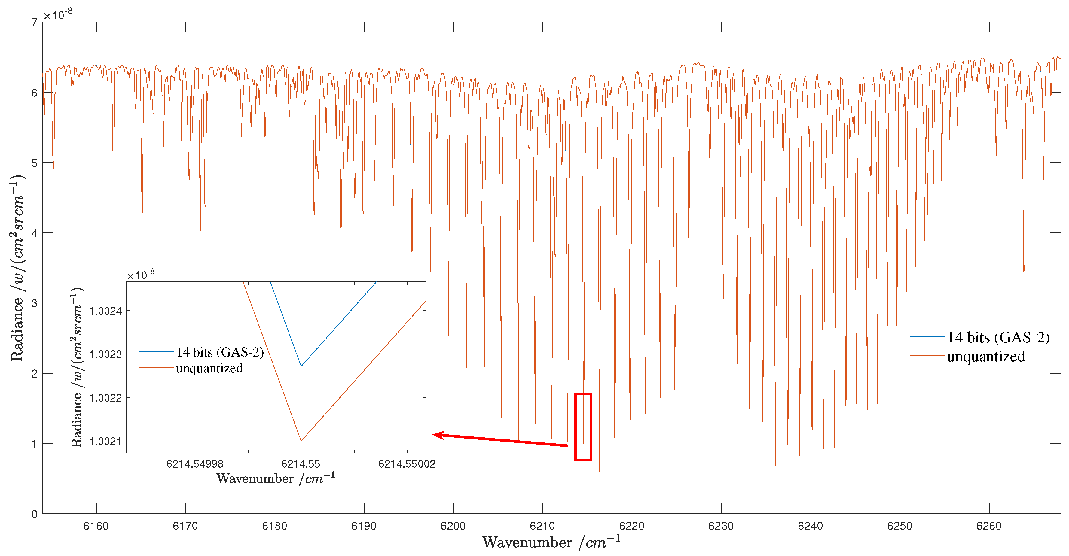
Radiometric resolution refers to the sensor’s ability to discern subtle changes in the radiative energy of ground objects, indicating its sensitivity. The higher radiometric resolution allows the sensor to detect smaller variations in the radiative energy emitted or reflected from the Earth’s surface. In other words, it represents the instrument’s ability to the smallest distinguishable difference in radiance when receiving spectral radiation signals. In remote sensing imagery, radiometric resolution is demonstrated by the quantization level assigned to each pixel’s radiance. This quantization level is typically represented by a sequence of grayscale values ranging from the brightest to the darkest. For GAS-2, the radiometric quantization is 14 bits, covering a range from 0 to 65535. The following Figure 9 illustrates the spectral radiance acquired by GAS-2 using its 14-bit radiometric quantization.

Figure 9 reveals that the quantization bits of GAS-2 can introduce errors in the acquired spectral radiance. According to the principles of analog-to-digital conversion, quantization bits inherently carry a bias known as the Least Significant Bit (LSB) error [62]. The LSB error arises because the Analog-to-Digital Converter (ADC) quantizes the continuous analog signal (radiance) into discrete digital levels based on the number of quantization bits. As a result, small variations in the analog signal that fall within one quantization level are approximated to the nearest digital level. This approximation introduces a systematic error into the digital representation of the analog signal, leading to the LSB error.

4.5. Simulation Results of Spectral Calibration Parameters

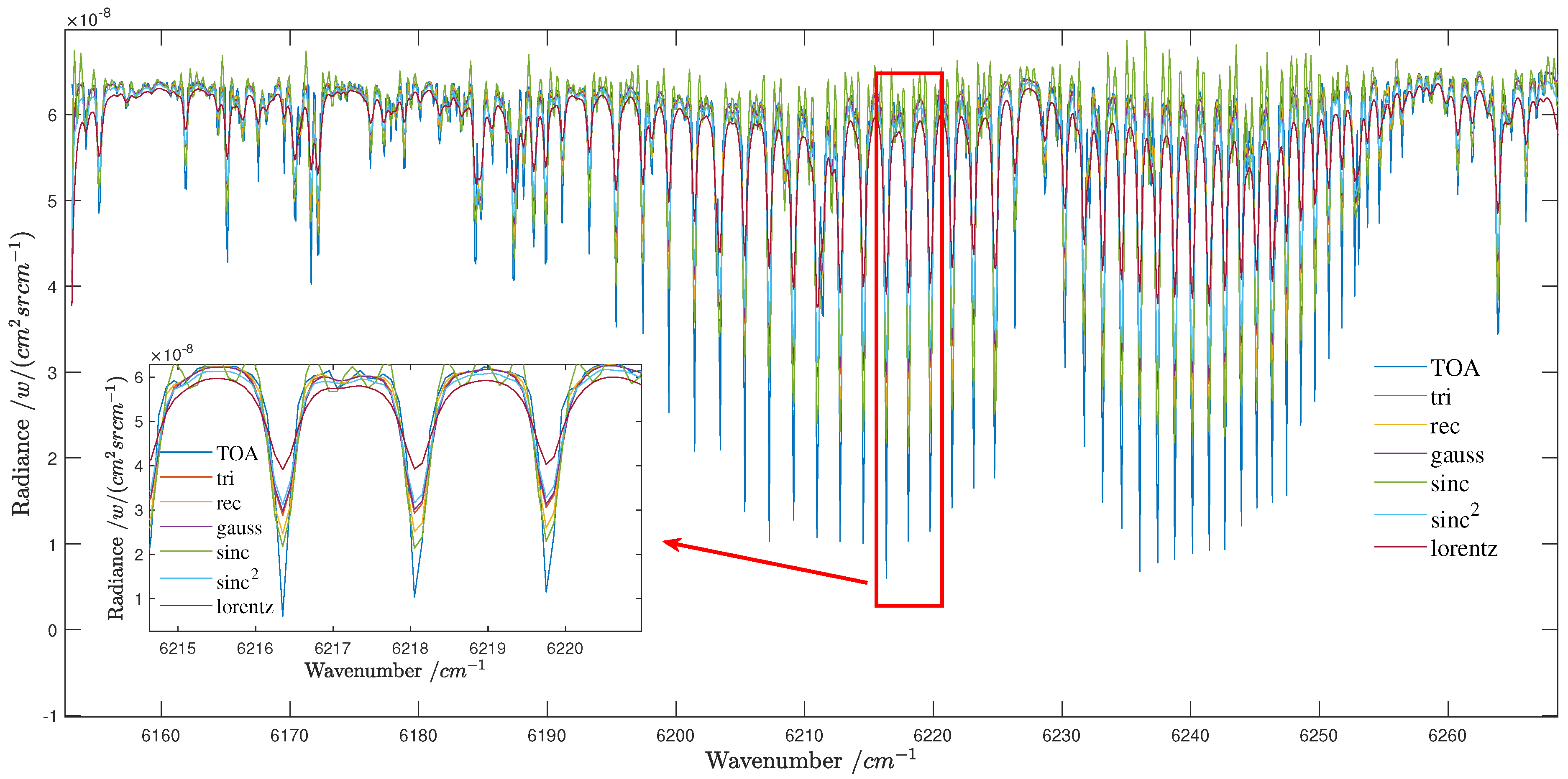
4.5.1. Simulation Results of Instrument Line Shape Functions

The Instrument Line Shape (ILS) function error in the instrument’s line shape function can introduce deviations in the measured radiance, which in turn may affect the retrieved CO${}_2$ concentration values. The determination of the instrument’s line shape function typically involves fitting it with a Gaussian function [63]. Nevertheless, it is essential to acknowledge that the true line shape function may not precisely follow a Gaussian distribution. In this section, we rigorously assess the instrument’s line shape function and explore the impact of various line-shape functions on GAS-2. Specifically, we examine the effects of trigonometric functions, rectangular functions, Gaussian functions, sinc functions, sinc${}^2$ functions, and Lorentzian functions [56]. GAS-2’s spectral resolution is finely set at 0.27 cm${}^{-1}$, and the simulations consider an atmospheric carbon dioxide concentration of 400 ppm. We employ the atmospheric top-of-atmosphere (TOA) spectral radiance as a reference and convolve it with different instrument line shape functions to derive the instrument-measured spectral radiance values, as depicted in the Figure 10.

The Figure 10 demonstrates that GAS-2’s instrument line shape function (ILS) has a discernible impact on the instrument-measured spectral radiance, even when the spectral resolution remains constant at 0.27 cm${}^{-1}$. During the inversion process, it is essential to consider the instrument’s ILS as it significantly influences the detection accuracy. Therefore, in this study, particular emphasis is placed on investigating the effect of ILS on the instrument’s performance. The discussion section provides a comprehensive and quantitative analysis of the impact of the ILS.

4.5.2. Simulation Results of Central Wavenumber Shift

The center wavelength of an instrument plays a crucial role in spectral calibration because determines the accuracy of the instrument’s measurements. Even if there is a deviation between the calibrated center wavelength and the actual center wavelength, the instrument can still sample the incident spectral radiance and acquire relevant information. However, when the calibrated center wavelength deviates from the actual value, it can introduce errors in the measured radiance, thus affecting the retrieval of greenhouse gas concentrations. In this section, we investigate the impact of center wavelength offset on GAS-2’s ability to measure spectral radiance. Specifically, we examine the effect of center wavelength offsets in the spectral calibration parameter of ILS, assuming offsets of 1%, 5%, 10%, 20%, and 30% of GAS-2’s spectral resolution (0.27 cm${}^{-1}$). The simulation results are illustrated in Figure 11.

Figure 11 provides clear evidence that the center wavenumber of the Instrument Line Shape (ILS) significantly affects the accuracy of the spectral positions acquired by GAS-2. Notably, deviations in the spectral position, particularly at the absorption peaks and valleys, can result in a decreased detection precision for GAS-2. This underscores the critical importance of carefully considering the influence of central wavenumber offsets. In the subsequent discussion section, we will delve into a quantitative analysis of the results related to this effect.

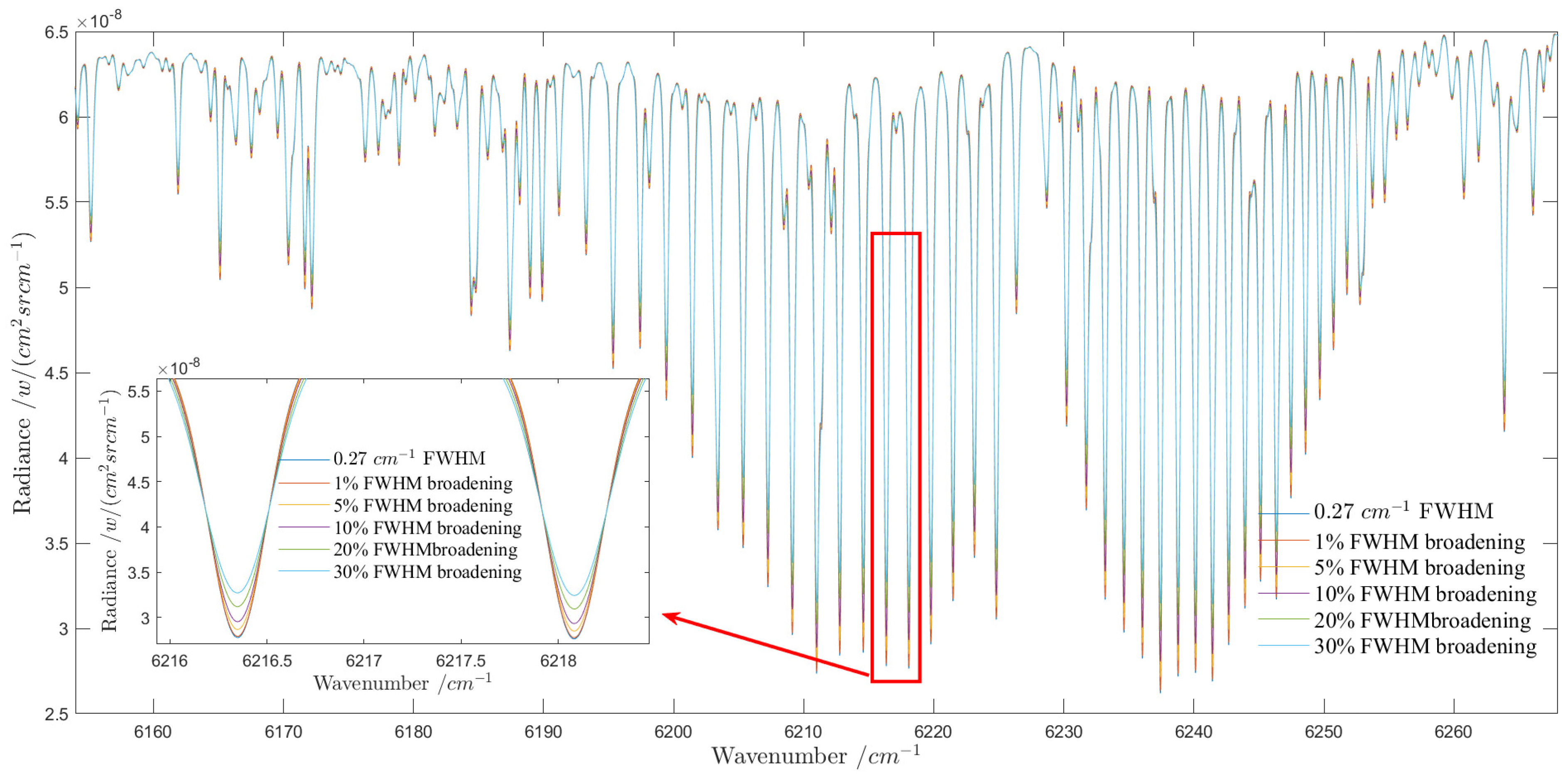
4.5.3. Simulation Results of Spectral Resolution Broadening

During practical spectral calibration, the instrument’s spectral resolution is typically determined by scanning a calibration light source with specific step sizes [64]. However, due to the finite linewidth of the calibration light source, the resulting spectral calibration exhibits an increase in spectral resolution. Despite this broadening effect, the instrument can still sample the incident spectral radiance and extract relevant information. Nevertheless, since the broadened spectral resolution is considered the actual resolution, it can introduce deviations in the retrieved radiance, thereby impacting the retrieval accuracy of greenhouse gas concentrations. In this section, we investigate the influence of spectral resolution on GAS-2’s acquisition of spectral radiance. GAS-2’s spectral resolution is 0.27 cm${}^{-1}$, and we explore the impact of broadening its resolution by 1%, 5%, 10%, 20%, and 30% to assess its effect on the instrument’s radiance retrieval. The simulation results are presented in Figure 12 below.

Based on Figure 12, it is evident that the broadening of spectral resolution has an impact on the spectral radiance acquired by GAS-2. Particularly, at the positions of absorption peaks and valleys, the broadening of spectral resolution leads to a decrease in GAS-2’s detection precision, underscoring the significance of considering the effects of spectral resolution broadening. This effect becomes particularly critical when monitoring the concentration of specific gases, such as greenhouse gases. To explore the influence of spectral resolution broadening on GAS-2’s performance, it is crucial to assess the instrument’s detection precision under different conditions. Consequently, the discussion section quantitatively analyzes the experimental results to reveal the specific impact of spectral resolution broadening on the measurement outcomes. By comprehensively comparing the data obtained at various levels of broadening, we can comprehensively evaluate GAS-2’s performance under different spectral resolution conditions, offering valuable insights for instrument optimization and practical application.

5. Discussion

5.1. Evaluation of the Performance of GSA-2 Instrument’s Parameters

5.1.1. Evaluation of Spectral Resolution

In the assessment of the GAS-2 instrument’s performance in the weak CO${}_2$ band, we have compiled the evaluation metrics in

Table 6. Evaluation factors of spectral resolution of GAS-2 and other loads with different spectral resolutions [15,58].

Payload	Spectral Resolution	Wavenumber Offset of the Lowest P-Branch (cm${}^{-1}$)	Wavenumber Offset of the Lowest R-Branch (cm${}^{-1}$)	RMSE	MAXAE	MEANAE	MAXRE (%)	MEANRE (%)
GAS-2/GOSAT	0.27	0.001	0.0134	0.0519	0.4140	0.0189	120.83	2.84
OCO-2	0.31	0.009	0.09	0.0594	0.5056	0.0221	172.1	3.32
ACGS (Tansat)	0.46	0.143	0.00537	0.0671	0.5300	0.0269	168.18	3.96

below. The reference point for these metrics is based on a CO${}_2$ absorption linewidth of 0.07 cm${}^{-1}$ [35]. A noteworthy observation from the table is that as the spectral resolution increases, the deviations in transmittance at the lowest points of the P and R branches decrease, and the root mean squared error (RMSE) also reduces. Additionally, the evaluation metrics, including mean relative error (MEANRE), mean absolute error (MEANAE), maximum relative error (MAXRE), and maximum absolute error (MAXAE), all demonstrate superior performance with higher spectral resolution. These findings underscore the importance of higher spectral resolution in achieving greater accuracy and precision in the retrieval of transmittance measurements.

GAS-2 is equipped with a grating spectrometer, which allows for a meaningful comparison with other similar grating-type payloads such as OCO-2 and TANSAT. Figure 13 illustrates the absolute deviation of transmittance spectra corresponding to different spectral resolutions for each payload. Our meticulous research reveals that GAS-2’s spectral resolution meets international standards and even surpasses those of existing payloads.

Through a comprehensive assessment of various evaluation metrics, it becomes evident that GAS-2’s transmittance spectra exhibit significantly smaller deviations when compared to those obtained by other payloads of similar characteristics. This performance accentuates GAS-2’s competitive edge, particularly in comparison to OCO-2. Consequently, the significance of GAS-2 as an invaluable instrument for atmospheric monitoring and precise greenhouse gas concentration retrieval is reinforced.

5.1.2. Evaluation of Spectral Sampling Rate

We conducted a comparative analysis of the spectral sampling rates of ACGS (TANSAT), OCO-2, and GAS-2 to evaluate the impact of spectral sampling rate on the detection accuracy of GAS-2. In this assessment, we used a spectral sampling rate of 6 as the reference value and introduced an additional spectral sampling rate of 1 as the comparative value. To quantify the level of deviation, we employed evaluation metrics such as Root Mean Square Error (RMSE), Absolute Error (AE), and Relative Error (RE). The evaluation results are presented in

Table 7. Evaluation factors of spectral sampling rate of GAS-2 and other loads with different spectral sampling rates [58,61].

Spectral Sampling Rate	Spectral Transmittance of the Lowest P-Branch (cm${}^{-1}$)	Spectral Transmittance of the Lowest R-Branch (cm${}^{-1}$)	RMSE	MAXAE	MEANAE	MAXRE (%)	MEANRE (%)
1	0.6616	0.6572	0.0137	0.1135	0.0053	21.20	0.62
2 (OCO-2)	0.7087	0.6572	0.0055	0.0671	0.0015	10.34	0.18
2.5 (ACGS)	0.6729	0.6297	0.0043	0.0549	0.0010	8.62	0.13
3 (GAS-2)	0.6561	0.6572	0.0033	0.0444	$7.469\times {10}^{-4}$	6.98	$8.9\times {10}^{-2}$

, and the absolute error is illustrated in Figure 14. These findings contribute to a more comprehensive understanding of the influence of spectral sampling rates on GAS-2’s detection precision and provide valuable insights for atmospheric monitoring and greenhouse gas concentration retrieval.

The analysis results in Table 7 highlight the influence of spectral sampling rate on detection accuracy. ACGS has a spectral sampling rate of 2, OCO-2 has a rate of 2.5, and GAS-2 has a rate of 3. Increasing the spectral sampling rate leads to reductions in RMSE, RE, and AE, resulting in enhanced detection precision. Furthermore, compared to spectral resolution, the impact of spectral sampling rate on detection accuracy is one order of magnitude smaller. The spectral sampling rate is closely related to the detector pixels. In the instrument design, GAS-2 employs 1304 detector pixels in the spectral dimension with a sampling rate of 3, while OCO-2 has 1024 detector pixels with a sampling rate of 2.5 [58], and Tansat has 500 detector pixels with a sampling rate of 2 [61]. When the spectral sampling rate reaches 3 (GAS-2), the RMSE is less than 0.0033 and the MEANRE is less than 0.1%, meeting the requirement for high detection accuracy.

Through the comprehensive analysis in this section, we have gained a thorough understanding of how the spectral sampling rate affects the measurement capability of GAS-2. The establishment of a quantitative relationship between sampling rate and measurement precision holds significant implications for advancing atmospheric sensing techniques. Moreover, it paves the way for enhanced data interpretation and analysis in future research, ultimately leading to more accurate and reliable insights into atmospheric composition and dynamics.

5.1.3. Evaluation of SNR

To assess the performance of GAS-2’s signal-to-noise ratio (SNR) metric, we compared it with two other grating spectrometer payloads, namely OCO-2 and ACGS (TANSAT). At typical energy levels, the SNR values for OCO-2, ACGS, and GAS-2 are 358, 250, and 340, respectively [65,66]. We first calculated the required SNR for detecting 1–4 ppm under typical energy conditions and then compared them with the set SNR values to verify if they meet the requirements. Specifically, at typical energy conditions, with a solar zenith angle of 60 degrees and a surface reflectance of 0.05 [65,66], the SNR values needed for detecting 1–4 ppm for OCO-2, ACGS, and GAS-2 are shown in

Table 8. SNR requirements of GAS-2 and other payloads under typical conditions [65,66].

Payload	ACGS (Tansat)	OCO-2	GAS-2
Spectral resolution (cm${}^{-\mathbf{1}}$)	0.46	0.31	0.27
Spectral range (nm)	1594–1624	1590–1621	1595–1625
SNR for 1 ppm	265	184	162
SNR for 2 ppm	133	92	81
SNR for 3 ppm	88	61	54
SNR for 4 ppm	66	46	40
SNR of payload	250	358	340

. All three payloads operate in similar spectral bands, each containing 31 absorption peaks and valleys. Consequently, the SNR requirements are derived for the 31 absorption peak-valley conditions.

Based on the data presented in Table 8, it is evident that GAS-2 demonstrates detection accuracy comparable to existing international instruments. The simulation results reveal that GAS-2 achieves an impressive detection accuracy of 1 ppm. Notably, OCO-2 and TANSAT are already in orbit, and publicly available literature indicates that OCO-2’s detection accuracy ranges between 1 and 2 ppm [67,68,69], while ACGS achieves a detection accuracy of 1 to 4 ppm [70].

When we consider the spectral and signal-to-noise ratio indicators of these instruments, GAS-2 exhibits a detection accuracy similar to that of OCO-2, approximately in the range of 1 to 2 ppm. However, it is important to bear in mind that these are preliminary simulated results, and the actual detection accuracy of GAS-2 needs to be further verified during its in-orbit operation.

The comparable performance of GAS-2 with well-established instruments such as OCO-2 and ACGS (TANSAT) underscores the significant advancements in atmospheric remote sensing technology. The potential 1 ppm detection accuracy of GAS-2 is highly promising and augments the capabilities of global greenhouse gas monitoring efforts.

5.1.4. Evaluation of Radiometric Resolution

GAS-2 has a radiation quantization bit depth of 14 bits.To assess the impact of GAS-2’s radiometric resolution (quantization bit depth) on the accuracy of spectral radiance, the unquantized spectral radiance is used as a reference to evaluate its precision effect. For a more comprehensive evaluation of the influence of GAS-2’s quantization bit depth, it can be compared with similar payloads such as GOSAT with a quantization bit depth of 16 bits [71], GOSAT-2, and ACGS with a quantization bit depth of 14 bits [12,61]. The results of absolute error and relative error are shown in Figure 15.

Based on the graph, it is evident that the error caused by the 16-bit quantization resolution (GOSAT) is smaller than that of the 14-bit resolution (GAS-2/ACGS/GOSAT-2). The root mean square error (RMSE) of the absolute error caused by 16-bit resolution is $1.5677\times {10}^{-13}$ W/(cm${}^2$· sr · cm${}^{-1}$), with a mean relative error (MEANAE) of $0.349\times {10}^{-13}$ W/(cm${}^2$· sr · cm${}^{-1}$). On the other hand, the RMSE of the absolute error caused by 14-bit resolution is $6.4954\times {10}^{-13}$ W/(cm${}^2$· sr · cm${}^{-1}$), with a MEANAE of $5.602\times {10}^{-13}$ W/(cm${}^2$· sr · cm${}^{-1}$). To assess the evaluation results of the errors caused by the 14-bit and 16-bit quantization resolutions, a comparison is made with a variation of 1 ppm in carbon dioxide concentration. The evaluation results are presented in

Table 9. Evaluation of errors caused by quantization bits [12,61,71].

Quantization Bits	RMSE (W/(cm${}^2$ · sr · cm${}^{-1}$))	MAXAE (W/(cm${}^2$ · sr · cm${}^{-1}$))	MEANAE (W/(cm${}^2$ · sr · cm${}^{-1}$))	MAXRE (%)	MEANRE (%)
14 (GAS-2/ACGS/GOSAT-2)	$6.495\times {10}^{-13}$	$1.098\times {10}^{-12}$	$5.602\times {10}^{-13}$	$3.329\times {10}^{-3}$	$9.985\times {10}^{-4}$
16 (GOSAT-1)	$1.568\times {10}^{-13}$	$2.745\times {10}^{-13}$	$1.349\times {10}^{-13}$	$8.282\times {10}^{-4}$	$2.106\times {10}^{-4}$
1 ppm change	$1.177\times {10}^{-11}$	$3.634\times {10}^{-11}$	$7.265\times {10}^{-12}$	$0.12$	$1.56\times {10}^{-2}$

below.

Based on Table 9, we can observe that the 14-bit quantization resolution results in an RMSE of about 5.5% for a 1 ppm concentration variation, with a MEANRE of approximately 6%. This corresponds to a detection precision error of around 0.05 ppm. On the other hand, the 16-bit quantization resolution yields an RMSE of about 1.3% and a MEANRE of approximately 1.54% for the same 1 ppm concentration variation, resulting in a detection precision error of about 0.01 ppm.

Considering the electronic bandwidth and data transmission rate, GAS-2’s decision to opt for a 14-bit quantization depth meets the required detection precision. While a higher quantization depth theoretically provides greater precision, it is crucial to strike a balance because higher quantization depths would necessitate higher instrument data transmission rates and electronic bandwidth. Therefore, GAS-2’s decision to use a 14-bit quantization depth is a well-considered and appropriate compromise, ensuring both accuracy and operational feasibility. The fact that GOSAT’s first-generation instrument employs a 16-bit quantization depth, while GOSAT-2 utilizes a 14-bit quantization depth, further validates the suitability of GAS-2’s 14-bit quantization depth for detection requirements. This comprehensive evaluation supports the efficacy of GAS-2’s instrument design in achieving accurate and reliable measurements for atmospheric monitoring and greenhouse gas concentration retrieval.

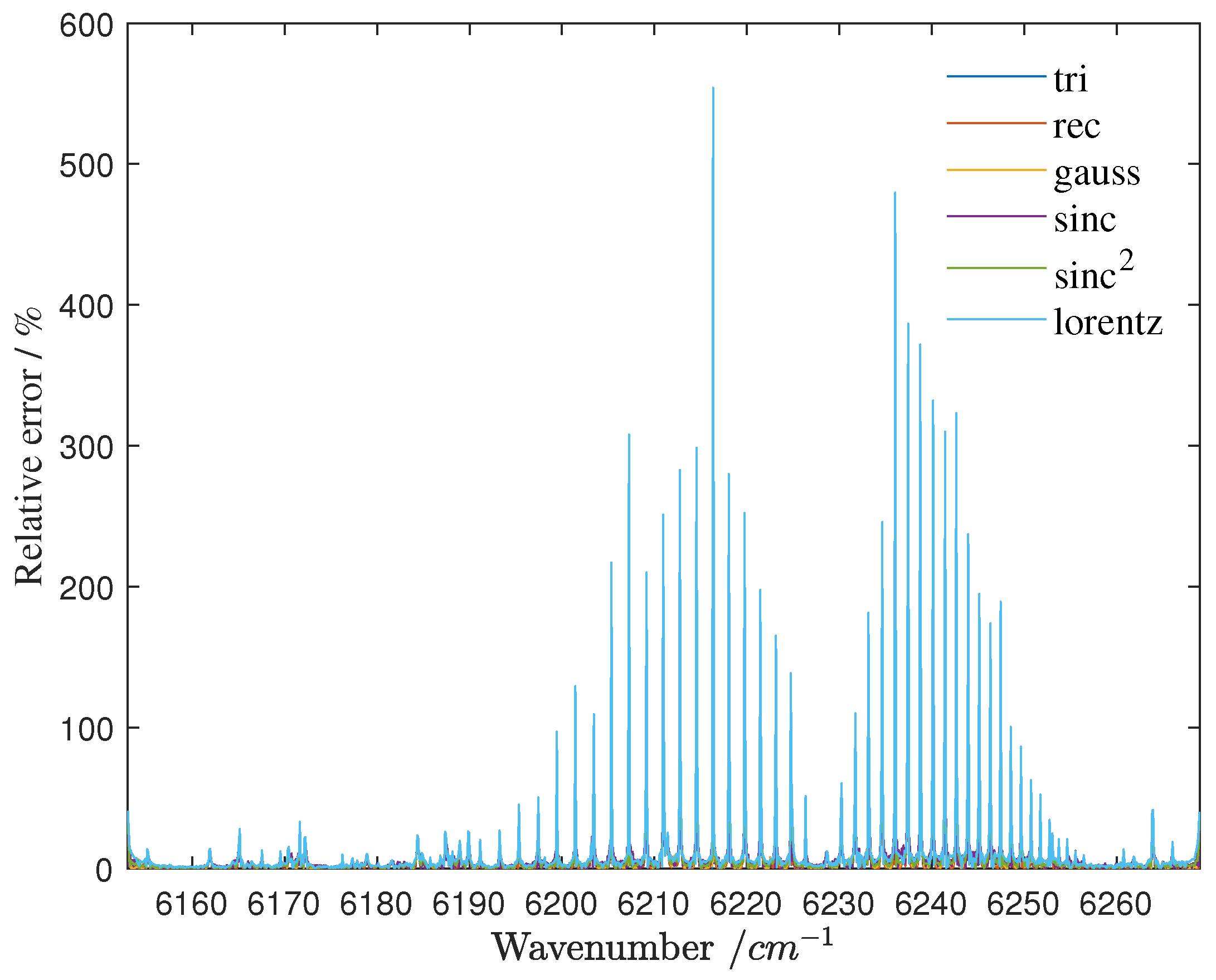
5.1.5. Evaluation of ILS

To quantitatively assess the instrument line shape (ILS) function of GAS-2, we compared the error between the radiance obtained using various ILS and the radiance resulting from the convolution at the top of the atmosphere (TOA). A smaller error indicates a higher degree of matching between the ILS and TOA radiance. The evaluation results for Relative Error (RE) are depicted in Figure 16, while additional indicators can be found in

Table 10. Errors of different instrument line shape functions at the same spectral resolution (0.27 cm${}^{-1}$) as GAS-2, with respect to TOA.

ILS	RMSE (W/(cm${}^2$ · sr · cm${}^{-1}$))	MAXAE (W/(cm${}^2$ · sr · cm${}^{-1}$))	MEANAE (W/(cm${}^2$ · sr · cm${}^{-1}$))	MAXRE (%)	MEANRE (%)
Tri	$4.527\times {10}^{-9}$	$2.307\times {10}^{-8}$	$2.467\times {10}^{-9}$	381.54	8.31
Rec	$3.675\times {10}^{-9}$	$2.173\times {10}^{-8}$	$1.895\times {10}^{-9}$	312.17	6.46
Gauss	$4.636\times {10}^{-9}$	$2.388\times {10}^{-8}$	$2.544\times {10}^{-9}$	396.81	8.59
Sinc	$4.102\times {10}^{-9}$	$2.022\times {10}^{-8}$	$2.716\times {10}^{-9}$	279.42	6.42
Sinc${}^2$	$4.786\times {10}^{-9}$	$2.528\times {10}^{-8}$	$2.716\times {10}^{-9}$	422.96	9.13
Lorentz	$6.385\times {10}^{-9}$	$3.312\times {10}^{-8}$	$3.856\times {10}^{-9}$	554.18	12.54

below.

The evaluation of different instrument line shape functions (ILS) in comparison with the top of the atmosphere (TOA) radiance highlights the presence of varying levels of error. Among the considered functions, the Root Mean Squared Error (RMSE) shows the following ordering from highest to lowest: Lorentz function, sinc${}^2$ function, Gaussian (Gauss) function, triangular (tri) function, rectangular (rec) function, and sinc function. These findings underscore the importance of carefully selecting the appropriate ILS to achieve accurate spectral radiance retrievals. Remarkably, when preserving the same spectral resolution as GAS-2 (0.27 cm${}^{-1}$), ILS based on sinc and rectangular functions demonstrate relatively smaller errors, making them more suitable for precise radiance retrieval. Conversely, the Lorentz function exhibits the highest error, suggesting potential limitations in its suitability for certain applications.

Furthermore, it is crucial to note that the errors associated with these ILS predominantly emerge at the peaks and valleys of carbon dioxide absorption in the spectral region under investigation. This observation is consistent with the nature of convolution, where the ILS function convolves with the underlying spectral features, influencing the accuracy of radiance measurements in those specific regions.

These findings provide valuable insights into the sensitivity of different ILS functions and their impact on the accuracy of radiance retrieval in the weak-CO2 spectral region. Understanding the behavior of these functions can aid in optimizing the instrument’s performance and calibration strategies, ultimately enhancing the precision of greenhouse gas concentration retrievals.

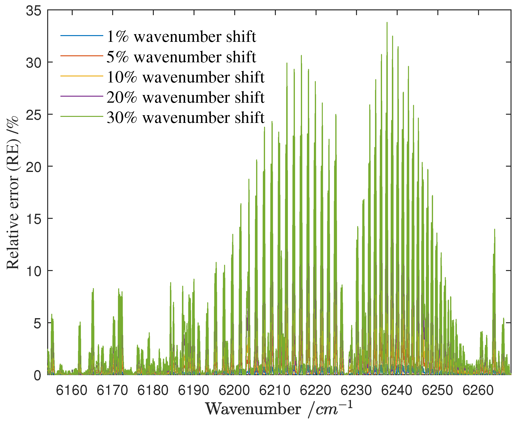
5.1.6. Evaluation of Central Wavenumber Shift

To evaluate the impact of center wavelength offsets, we utilized a method that compares radiance data obtained without any center wavelength shift as a reference. Subsequently, we introduced various center wavelength displacements to analyze their effects. During this evaluation, we employed several key metrics, including Root Mean Squared Error (RMSE), absolute error, and relative error, to precisely quantify the deviations caused by the center wavelength offsets. These evaluation metrics provide valuable insights into the magnitude of deviations resulting from center wavelength shifts and help us understand their influence on the accuracy of greenhouse gas concentration retrievals. The Relative Error (RE) is graphically depicted in Figure 17, and further metrics are available in

Table 11. Errors of GAS-2 caused by different center wavenumber shifts (weak-CO${}_2$ band).

Wavenumber shift/SR * (%)	RMSE (W/(cm${}^2$ · sr · cm${}^{-1}$))	MEANAE (W/(cm${}^2$ · sr · cm${}^{-1}$))	MAXAE (W/(cm${}^2$ · sr · cm${}^{-1}$))	MAXRE (%)	MEANRE (%)
1	$1.0376\times {10}^{-10}$	$6.393\times {10}^{-11}$	$3.693\times {10}^{-10}$	1.009	0.133
5	$5.1851\times {10}^{-10}$	$3.193\times {10}^{-10}$	$1.845\times {10}^{-9}$	5.143	0.665
10	$1.0354\times {10}^{-9}$	$6.372\times {10}^{-10}$	$3.683\times {10}^{-9}$	10.518	1.327
20	$2.0576\times {10}^{-8}$	$1.266\times {10}^{-9}$	$7.307\times {10}^{-8}$	21.870	2.634
30	$3.0539\times {10}^{-8}$	$1.879\times {10}^{-9}$	$1.081\times {10}^{-8}$	33.810	3.108

* SR is the spectral resolution of this band of GAS-2.

.

As presented in Table 11, the degree of spectral calibration center wavelength shift significantly affects the precision of spectral radiance retrieval conducted by the instrument. Larger shifts in wavelength are associated with increased errors and reduced accuracy in acquiring radiance data. Notably, even a minor 1% shift in the center wavelength results in an average relative error of 0.1% in spectral radiance. Therefore, meticulous attention to spectral calibration becomes paramount, ensuring the precise determination of the center wavelength response for each pixel within GAS-2. This underscores the heightened requirements for calibration light sources and calibration techniques.

These compelling findings offer strong evidence that minimizing center wavelength shifts can effectively reduce errors and enhance the accuracy of acquired data. The observed outcomes underscore the criticality of precise calibration and diligent maintenance of the instrument’s center wavelength. Such measures hold utmost significance in guaranteeing trustworthy and precise measurement of spectral radiance, thereby enabling the exact retrieval of greenhouse gas concentrations. The emphasis on sustaining a stable center wavelength cannot be overstressed, particularly when striving for dependable and resilient outcomes in atmospheric research and greenhouse gas monitoring.

5.1.7. Evaluation of FWHM Broading

We conducted a quantitative assessment of how spectral broadening parameters affect the accuracy of spectral radiance retrieval in GAS-2. To establish a reference, we utilized the original spectral resolution without any broadening effect and then quantified the impact of different spectral broadening values. During the evaluation, we employed various metrics such as Root Mean Squared Error (RMSE), Absolute Error (AE), and Relative Error (RE) to quantify the extent of their influence. Figure 18 illustrates the relative errors in spectral radiance retrieval caused by varying spectral broadening parameters in GAS-2. Additionally, other evaluation metrics can be found in

Table 12. Errors of GAS-2 caused by different degrees of spectral resolution broadening.

Spectral Resolution Broadening/SR * (%)	RMSE (W/(cm${}^2$ · sr · cm${}^{-1}$)	MEANAE (W/(cm${}^2$ · sr · cm${}^{-1}$)	MAXAE (W/(cm${}^2$ · sr · cm${}^{-1}$)	MAXRE (%)	MEANRE (%)
1	$3.186\times {10}^{-11}$	$1.904\times {10}^{-11}$	$1.499\times {10}^{-10}$	0.57	0.041
5	$2.044\times {10}^{-10}$	$1.226\times {10}^{-10}$	$9.570\times {10}^{-10}$	3.65	0.267
10	$4.025\times {10}^{-10}$	$2.425\times {10}^{-10}$	$1.874\times {10}^{-9}$	7.15	0.527
20	$7.939\times {10}^{-10}$	$4.826\times {10}^{-10}$	$3.653\times {10}^{-9}$	13.95	1.045
30	$1.159\times {10}^{-9}$	$7.104\times {10}^{-9}$	$5.275\times {10}^{-9}$	20.14	1.535

* SR is the spectral resolution of this band of GAS-2.

.

As shown in Figure 18 and Table 12, the observed broadening of spectral resolution has a significant impact on the accuracy of spectral radiance inversion, consequently affecting the precision of greenhouse gas detection. In the weak CO${}_2$ band, with an initial spectral resolution of 0.27 cm${}^{-1}$, we examined its effects under different broadening percentages and found that higher broadening percentages result in more pronounced errors and substantial influences on measurements. For instance, when the spectral resolution is broadened by 1%, we observed an average relative error of 0.04% in the instrument-retrieved radiance. The higher the resolution broadening, the greater the errors in the instrument-retrieved spectral radiance. The primary sources of spectral resolution broadening during calibration are the linewidth of the calibration light source and the spectral fitting algorithm, which necessitates narrower linewidth calibration light sources and appropriate algorithms to ensure minimal spectral resolution broadening.

The impact of spectral resolution broadening on the acquired spectral information is a crucial consideration for accurate measurement and analysis. Expanding the spectral resolution compromises the instrument’s ability to resolve fine spectral details, resulting in a broader representation of spectral features. This leads to a loss in spectral accuracy, affecting the identification and quantification of specific features, such as greenhouse gas absorption lines. Advanced calibration techniques and data processing algorithms are vital in addressing these challenges. The OCO and OCO-2 missions employ laser-based spectral measurements prior to launch to determine the instrument linear (ILS) function and dispersion parameters. Ensuring the accuracy of spectral calibration, the OCO mission selects a tunable laser with a linewidth better than 1 MHz [72], while OCO-2 requires a tunable laser with a linewidth better than 300 KHz [64]. Additionally, both missions impose corresponding requirements on wavelength stability to guarantee precise and reliable spectral calibration.

5.2. The Sources of Errors in Instrument Parameters

GAS-2 is a push-broom imaging spectrometer that employs a grating for spectral dispersion. This study emphasizes the quantitative impact of instrument parameters on the detection performance of GAS-2. The sources of errors in these instrument parameters also require detailed analysis and quantification. The errors in spectral resolution may originate from factors such as the number of grooves on the grating, precision of optical components, mechanical imperfections during manufacturing, optical element instability, instrument sensitivity to temperature or humidity, and inaccuracies in calibration. These factors can lead to deviations in the spectral resolution. The spectral sampling rate refers to the density of spectral samples in wavenumber or wavelength. It is closely related to the number of detector pixels. Higher sampling rates require more detector pixels, but excessively high sampling rates should be avoided due to constraints imposed by the signal-to-noise ratio, necessitating a balanced approach in selecting an appropriate rate. Radiance quantization bit-depth is primarily limited by the number of bits in the analog-to-digital converter (ADC), and the precision can be affected by electronic component noise. The signal-to-noise ratio is the ratio of the instrument’s measured signal to background noise. The sources of errors in the signal-to-noise ratio include variations in optical component transmittance, noise from optical elements and detectors, and electronic circuit noise, which can impact its stability and accuracy. The instrument linearity function represents the instrument’s response to light intensity at different wavelengths. The sources of errors in the instrument linearity function mainly stem from non-uniformity in optical elements and nonlinearity in the optical system. Moreover, errors in the characterization of the instrument linearity function also include light source selection and data processing. Regarding spectral calibration, errors in the center wavelength shift and spectral broadening mainly originate from the precision of the calibration instrument, such as the wavelength stability and accuracy of the calibration light source, the linewidth of the light source, and data processing during spectral calibration. Quantifying these error sources is one of the key directions for future research.

5.3. Limitations and Future Research Directions

Although this study provides valuable insights into the sensitivity of GAS-2 instrument parameters to detecting atmospheric greenhouse gas concentration changes, it is essential to acknowledge its inherent limitations. Firstly, the quantitative analysis is based on the US Standard Atmosphere model, which itself deviates from the actual atmospheric conditions. However, as a representative input for research purposes, it provides a reasonable approximation to elucidate the research question. Secondly, this study relies on atmospheric radiative transfer models. Different atmospheric transfer models may yield diverse results, thereby limiting the universality of the research findings. Nonetheless, despite variations in transfer models, the study’s tools demonstrate that the impact of instrument parameters on atmospheric greenhouse gas concentration changes is acceptable. Thirdly, when studying the effects of individual instrument parameters on atmospheric greenhouse gas concentration, this research assumes ideal and constant atmospheric and surface conditions, which may deviate from real-world conditions. It is imperative to underscore that the precision of atmospheric CO${}_2$ concentration measurements is subject to the intricate interplay of various factors, encompassing real atmospheric conditions, instrument parameters, data quality, ground-based verification, and inversion methodologies. This amalgamation constitutes a comprehensive systemic challenge. Central to the current study is an in-depth exploration into the impact of GAS-2’s instrument parameters on the accuracy of acquiring atmospheric GHG concentrations. To rigorously address this focus, a meticulous control variable strategy is employed to effectively manage and account for the potential influence of the other multifaceted factors at play. Thus, this study inherently has limitations. Additionally, due to the ongoing development of GAS-2, the effective validation of sensitivity analysis is constrained.

This study focuses on investigating the sensitivity of instrument parameters obtained from GAS-2 to atmospheric greenhouse gas concentration changes. It is well-known that the accuracy of carbon dioxide concentration measurements in the atmosphere is influenced by a combination of atmospheric parameters, instrument parameters, and inversion strategies. To more accurately assess the impact of GAS-2 on retrieving atmospheric greenhouse gas concentrations, further research is necessary to investigate the influence of various atmospheric parameters. For instance, a detailed examination of significant atmospheric aerosol parameters (AOD) should be conducted to understand their impact on GAS-2’s sensitivity to atmospheric greenhouse gas concentrations. The vertical profiles of temperature and humidity, cloud characteristics, and surface albedo are also critical factors that require in-depth analysis to enhance greenhouse gas detection. Studying the complex relationship between these parameters and GAS-2 sensitivity will contribute to a comprehensive understanding of the detection process. Moreover, quantifying the sources of errors in instrument parameters is also a future research direction.

In conclusion, the findings of this study provide valuable guidance and reference for the construction of GAS-2, aiding in optimizing instrument design parameters and enhancing detection accuracy. In the future, expanding the scope of research, analyzing and quantifying the sources of instrument parameter errors, investigating the impact of atmospheric parameters (aerosols, temperature, humidity, etc.), data quality, ground-based verification and inversion algorithms on GAS-2’s accuracy in retrieving atmospheric greenhouse gases will pave the way for precise greenhouse gas detection.

6. Conclusions

In this research, we have meticulously investigated the influence of instrument parameters on the performance of GAS-2 in detecting atmospheric greenhouse gas concentrations. Our focus encompassed spectral resolution, spectral sampling rate, signal-to-noise ratio, radiance resolution, and spectral calibration parameters, including instrument line shape function, center wavelength offset, and spectral resolution broadening. Our analysis led to the following key conclusions:

• Spectral resolution: increasing spectral resolution enhances GAS-2’s ability to measure greenhouse gas total columns. A finer resolution provides comprehensive radiance information, boosting accuracy. GAS-2’s 0.27 cm${}^{-1}$ resolution ranks competitively on a global scale.
• Spectral sampling rate: the spectral sampling rate significantly influences radiance capture. A rating of 3 balances accuracy and practicality. GAS-2’s spectral sampling rate of 3 is an advanced level among similar international payloads.
• Signal-to-noise ratio (SNR): GAS-2’s 0.27 cm${}^{-1}$ resolution at typical energy meets the 1 ppm precision standards.
• Radiance resolution: greater radiance resolution improves accuracy. GAS-2’s 14-bit quantization depth surpasses the 1 ppm concentration variation accuracy by an order of magnitude.
• Spectral calibration: precise calibration bolsters accuracy. Different line shape functions impact radiance; the sinc function shows the least convolved error with TOA. Center wavelength offset and spectral resolution broadening significantly influence radiance.

In conclusion, our study provides a quantitative assessment of the impact of instrument parameters on the accuracy of GAS-2 in monitoring GHGs. By addressing the gaps in existing research, we underscore the significance of instrument parameters. These insights not only offer avenues for optimizing the design of similar payloads for GAS-2 but also deepen our comprehension of how instrument parameters influence GHG concentration detection. Furthermore, our findings hold the potential to guide and inform laboratory-based spectral calibration efforts for GAS-2.

References

1. Von Weizsacker, E.U.; Hargroves, C.; Smith, M.H.; Desha, C.; Stasinopoulos, P. Factor Five: Transforming the Global Economy through 80% Improvements in Resource Productivity; Routledge: London, UK, 2009. [Google Scholar]
2. Kenedi, K. The Effect of Energy Consumption and Taxes with the Mediation of Economic Growth on Pollution in 9 ASEAN Countries. Bina Bangsa Int. J. Bus. Manag. 2021, 1, 233–243. [Google Scholar]
3. Crist, E. Beyond the climate crisis: A critique of climate change discourse. Telos 2007, 141, 29–55. [Google Scholar]
4. Sterman, J.D.; Sweeney, L.B. Cloudy skies: Assessing public understanding of global warming. Syst. Dyn. Rev. J. Syst. Dyn. Soc. 2002, 18, 207–240. [Google Scholar] [CrossRef]
5. Ciais, P.; Dolman, A.J.; Bombelli, A.; Duren, R.; Peregon, A.; Rayner, P.J.; Miller, C.; Gobron, N.; Kinderman, G.; Marland, G.; et al. Current systematic carbon-cycle observations and the need for implementing a policy-relevant carbon observing system. Biogeosciences 2014, 11, 3547–3602. [Google Scholar] [CrossRef]
6. Hungershoefer, K.; Breon, F.M.; Peylin, P.; Chevallier, F.; Rayner, P.; Klonecki, A.; Houweling, S.; Marshall, J. Evaluation of various observing systems for the global monitoring of CO2 surface fluxes. Atmos. Chem. Phys. 2010, 10, 10503–10520. [Google Scholar] [CrossRef]
7. Luo, H.; Li, Z.; Wu, Y.; Qiu, Z.; Shi, H.; Wang, Q.; Xiong, W. Greenhouse Gases Monitoring Instrument on GaoFen-5 Satellite-II: Optical Design and Evaluation. Remote Sens. 2023, 15, 1105. [Google Scholar] [CrossRef]
8. Bovensmann, H.; Burrows, J.; Buchwitz, M.; Frerick, J.; Noel, S.; Rozanov, V.; Chance, K.; Goede, A. SCIAMACHY: Mission objectives and measurement modes. J. Atmos. Sci. 1999, 56, 127–150. [Google Scholar] [CrossRef]
9. Aumann, H.H.; Chahine, M.T.; Gautier, C.; Goldberg, M.D.; Kalnay, E.; McMillin, L.M.; Revercomb, H.; Rosenkranz, P.W.; Smith, W.L.; Staelin, D.H.; et al. AIRS/AMSU/HSB on the Aqua mission: Design, science objectives, data products, and processing systems. IEEE Trans. Geosci. Remote Sens. 2003, 41, 253–264. [Google Scholar] [CrossRef]
10. Blumstein, D.; Chalon, G.; Carlier, T.; Buil, C.; Hebert, P.; Maciaszek, T.; Ponce, G.; Phulpin, T.; Tournier, B.; Simeoni, D.; et al. IASI instrument: Technical overview and measured performances. Infrared Spaceborne Remote Sens. XII 2004, 5543, 196–207. [Google Scholar]
11. Guanter, L.; Frankenberg, C.; Dudhia, A.; Lewis, P.E.; Gómez-Dans, J.; Kuze, A.; Suto, H.; Grainger, R.G. Retrieval and global assessment of terrestrial chlorophyll fluorescence from GOSAT space measurements. Remote Sens. Environ. 2012, 121, 236–251. [Google Scholar] [CrossRef]
12. Suto, H.; Kataoka, F.; Kikuchi, N.; Knuteson, R.O.; Butz, A.; Haun, M.; Buijs, H.; Shiomi, K.; Imai, H.; Kuze, A. Thermal and near-infrared sensor for carbon observation Fourier transform spectrometer-2 (TANSO-FTS-2) on the Greenhouse gases Observing SATellite-2 (GOSAT-2) during its first year in orbit. Atmos. Meas. Tech. 2021, 14, 2013–2039. [Google Scholar] [CrossRef]
13. Bi, Y.; Zhang, P.; Yang, Z.; Wang, Q.; Zhang, X.; Liu, C.; Xu, P.; Hou, L.; Ke, J.; Zhang, N. Fast CO2 Retrieval Using a Semi-Physical Statistical Model for the High-Resolution Spectrometer on the Fengyun-3D Satellite. J. Meteorol. Res. 2022, 36, 374–386. [Google Scholar] [CrossRef]
14. Crisp, D.; Pollock, H.R.; Rosenberg, R.; Chapsky, L.; Lee, R.A.; Oyafuso, F.A.; Frankenberg, C.; O’Dell, C.W.; Bruegge, C.J.; Doran, G.B.; et al. The on-orbit performance of the Orbiting Carbon Observatory-2 (OCO-2) instrument and its radiometrically calibrated products. Atmos. Meas. Tech. 2017, 10, 59–81. [Google Scholar] [CrossRef]
15. Yang, Z.; Zhen, Y.; Yin, Z.; Lin, C.; Bi, Y.; Liu, W.; Wang, Q.; Wang, L.; Gu, S.; Tian, L. Laboratory spectral calibration of the TanSat atmospheric carbon dioxide grating spectrometer. Geosci. Instrum. Methods Data Syst. 2018, 7, 245–252. [Google Scholar] [CrossRef]
16. Eldering, A.; Taylor, T.E.; O’Dell, C.W.; Pavlick, R. The OCO-3 mission: Measurement objectives and expected performance based on 1 year of simulated data. Atmos. Meas. Tech. 2019, 12, 2341–2370. [Google Scholar] [CrossRef]
17. Shi, H.; Li, Z.; Ye, H.; Luo, H.; Xiong, W.; Wang, X. First level 1 product results of the greenhouse gas monitoring instrument on the GaoFen-5 satellite. IEEE Trans. Geosci. Remote Sens. 2020, 59, 899–914. [Google Scholar] [CrossRef]
18. Meng, G.; Wen, Y.; Zhang, M.; Gu, Y.; Xiong, W.; Wang, Z.; Niu, S. The status and development proposal of carbon sources and sinks monitoring satellite system. Carbon Neutrality 2022, 1, 32. [Google Scholar] [CrossRef]
19. Sun, X.; Kolbeck, P.T.; Abshire, J.B.; Kawa, S.R.; Mao, J. Attenuated atmospheric backscatter profiles measured by the CO2 Sounder lidar in the 2017 ASCENDS/ABoVE airborne campaign. Earth Syst. Sci. Data 2022, 14, 3821–3833. [Google Scholar] [CrossRef]
20. Amediek, A.; Fix, A.; Ehret, G.; Caron, J.; Durand, Y. Airborne lidar reflectance measurements at 1.57 μm in support of the A-SCOPE mission for atmospheric CO2. Atmos. Meas. Tech. 2009, 2, 755–772. [Google Scholar] [CrossRef]
21. Uprety, D.C.; Reddy, V.; Mura, J.D.; Uprety, D.C.; Reddy, V.; Mura, J.D. Greenhouse gases: A historical perspective. Clim. Chang. Agric. A Hist. Anal. 2019, 31–41. [Google Scholar]
22. Dubovik, O.; Li, Z.; Mishchenko, M.I.; Tanré, D.; Karol, Y.; Bojkov, B.; Cairns, B.; Diner, D.J.; Espinosa, W.R.; Goloub, P.; et al. Polarimetric remote sensing of atmospheric aerosols: Instruments, methodologies, results, and perspectives. J. Quant. Spectrosc. Radiat. Transf. 2019, 224, 474–511. [Google Scholar] [CrossRef]
23. Zhang, Y.; Li, Z.; Bai, K.; Wei, Y.; Xie, Y.; Zhang, Y.; Ou, Y.; Cohen, J.; Zhang, Y.; Peng, Z.; et al. Satellite remote sensing of atmospheric particulate matter mass concentration: Advances, challenges, and perspectives. Fundam. Res. 2021, 1, 240–258. [Google Scholar] [CrossRef]
24. Zhang, X.-Y.; Meng, X.-Y.; Zhou, M.-Q.; Bai, W.-G.; Zhou, L.-H.; Hu, Y.-M.; Yu, X. Review of the validation of atmospheric CO2 from satellite hyper spectral remote sensing. Adv. Clim. Chang. Res. 2018, 14, 602. [Google Scholar]
25. Li, Q.; Wang, X.; Ye, H.; Wu, S. Atmospheric CO2 Inversion Error Analysis and Accuracy Verification. Acta Opt. Sin. 2020, 40, 0601003. [Google Scholar]
26. Wu, J.; Wang, X.H.; Fang, Y.H.; Xiong, W.; Shi, H.; Qiao, Y. Ability analysis of spatial heterodyne spectrometer in atmospheric CO2 detection. Acta Opt. Sin. 2011, 31, 0101001. [Google Scholar]
27. Ye, H.-H.; Wang, X.-H.; Wu, J.; Fang, Y.-H. Sensitivity for retrieval of atmospheric column carbon dioxide with high accuracy. J. Atmos. Environ. Opt. 2011, 6, 208. [Google Scholar]
28. Yoshida, Y.; Kikuchi, N.; Morino, I.; Uchino, O.; Oshchepkov, S.; Bril, A.; Saeki, T.; Schutgens, N.; Toon, G.; Wunch, D.; et al. Improvement of the retrieval algorithm for GOSAT SWIR XCO2 and XCH4 and their validation using TCCON data. Atmos. Meas. Tech. 2013, 6, 1533–1547. [Google Scholar] [CrossRef]
29. Morino, I.; Uchino, O.; Inoue, M.; Yoshida, Y.; Yokota, T.; Wennberg, P.; Toon, G.; Wunch, D.; Roehl, C.; Notholt, J.; et al. Preliminary validation of column-averaged volume mixing ratios of carbon dioxide and methane retrieved from GOSAT short-wavelength infrared spectra. Atmos. Meas. Tech. Discuss. 2010, 3, 5613–5643. [Google Scholar] [CrossRef]
30. Connor, B.J.; Boesch, H.; Toon, G.; Sen, B.; Miller, C.; Crisp, D. Orbiting Carbon Observatory: Inverse method and prospective error analysis. J. Geophys. Res. Atmos. 2008, 113, D05305. [Google Scholar] [CrossRef]
31. Inoue, M.; Morino, I.; Uchino, O.; Miyamoto, Y.; Yoshida, Y.; Yokota, T.; Machida, T.; Sawa, Y.; Matsueda, H.; Sweeney, C.; et al. Validation of XCO2 derived from SWIR spectra of GOSAT TANSO-FTS with aircraft measurement data. Atmos. Chem. Phys. 2013, 13, 9771–9788. [Google Scholar] [CrossRef]
32. Cogan, A.; Boesch, H.; Parker, R.; Feng, L.; Palmer, P.; Blavier, J.F.; Deutscher, N.M.; Macatangay, R.; Notholt, J.; Roehl, C.; et al. Atmospheric carbon dioxide retrieved from the Greenhouse gases Observing SATellite (GOSAT): Comparison with ground-based TCCON observations and GEOS-Chem model calculations. J. Geophys. Res. Atmos. 2012, 117, D21301. [Google Scholar] [CrossRef]
33. Clough, S.A.; Iacono, M.J.; Moncet, J.L. LBLRTM: Line-By-Line Radiative Transfer Model; ascl: 1405.001; Astrophysics Source Code Library: Houghton, MI, USA, 2014. [Google Scholar]
34. Wang, Y.-R.; Xu, Q.-S.; Wei, H.-L. Influence of Improved MODTRAN5 Band Model Spectral Resolution on Background Radiation Calculation in Molecular Absorption Region. J. Atmos. Environ. Opt. 2015, 10, 205. [Google Scholar]
35. Mao, J.; Kawa, S.R. Sensitivity studies for space-based measurement of atmospheric total column carbon dioxide by reflected sunlight. Appl. Opt. 2004, 43, 914–927. [Google Scholar] [CrossRef] [PubMed]
36. Li, S.; Cheng, L.; Yang, H.; Ding, L.; Wang, X. Evaluation of the Accuracy of Spectral Calibration Light Source on Spectral Radiance Acquired by the Greenhouse-Gases Absorption Spectrometer-2 (GAS-2). Remote Sens. 2023, 15, 2636. [Google Scholar] [CrossRef]
37. Jin, J.; Henzing, B.; Segers, A. How aerosol size matters in aerosol optical depth (AOD) assimilation and the optimization using the Ångström exponent. Atmos. Chem. Phys. 2023, 23, 1641–1660. [Google Scholar] [CrossRef]
38. Islam, T.; Hu, Y.; Kokhanovsky, A.A.; Wang, J. Remote Sensing of Aerosols, Clouds, and Precipitation; Elsevier: Amsterdam, The Netherlands, 2017. [Google Scholar]
39. Schneising, O.; Buchwitz, M.; Burrows, J.; Bovensmann, H.; Reuter, M.; Notholt, J.; Macatangay, R.; Warneke, T. Three years of greenhouse gas column-averaged dry air mole fractions retrieved from satellite—Part 1: Carbon dioxide. Atmos. Chem. Phys. 2008, 8, 3827–3853. [Google Scholar] [CrossRef]
40. Oyafuso, F.; Payne, V.H.; Drouin, B.J.; Devi, V.M.; Benner, D.C.; Sung, K.; Yu, S.; Gordon, I.E.; Kochanov, R.; Tan, Y.; et al. High accuracy absorption coefficients for the Orbiting Carbon Observatory-2 (OCO-2) mission: Validation of updated carbon dioxide cross-sections using atmospheric spectra. J. Quant. Spectrosc. Radiat. Transf. 2017, 203, 213–223. [Google Scholar] [CrossRef]
41. Crisp, D.; Miller, C.E.; DeCola, P.L. NASA Orbiting Carbon Observatory: Measuring the column averaged carbon dioxide mole fraction from space. J. Appl. Remote Sens. 2008, 2, 023508. [Google Scholar] [CrossRef]
42. Song, W.; Jin, Y.; Zhao, Z.; Shen, W.; Fan, D. Analysis and Optical Design of Very High Spectral Resolution Imaging Spectrometer of the Atmospheric CO2. Acta Opt. Sin. 2015, 35, 271–281. [Google Scholar]
43. Boesch, H.; Brown, L.; Castano, R.; Christi, M.; Crisp, D.; Eldering, A.; Fisher, B.; Frankenberg, C.; Gunson, M.; Granat, R.; et al. Orbiting carbon observatory (OCO)-2 level 2 full physics retrieval algorithm theoretical basis. In Jet Propulsion Laboratory Technical Document; D-55207, Version; Laboratory California Institute of Technology: Pasadena, CA, USA, 2015; Volume 3. [Google Scholar]
44. Wang, Q.; Yang, Y.-D.; Bi, Y.M. Spectral parameters and signal-to-noise ratio requirement for CO2 hyper spectral remote sensor. J. Appl. Meteorol. Sci. 2014, 25, 600–609. [Google Scholar]
45. Ye, H.H.; Wang, X.H.; Wu, J.; Fang, Y.H.; Ma, J.J.; Jiang, X.H.; Wei, Q.Y. Study of the effect of surface reflectance on atmospheric CO2 retrieval and ratio spectrometry. Spectrosc. Spectr. Anal. 2013, 33, 2182–2187. [Google Scholar]
46. Rodgers, C.D. Inverse Methods for Atmospheric Sounding: Theory and Practice; World Scientific: Singapore, 2000; Volume 2. [Google Scholar]
47. Hobbs, J.M.; Drouin, B.J.; Oyafuso, F.; Payne, V.H.; Gunson, M.R.; McDuffie, J.; Mlawer, E.J. Spectroscopic uncertainty impacts on OCO-2/3 retrievals of XCO2. J. Quant. Spectrosc. Radiat. Transf. 2020, 257, 107360. [Google Scholar] [CrossRef]
48. Bösch, H.; Toon, G.; Sen, B.; Washenfelder, R.; Wennberg, P.; Buchwitz, M.d.; De Beek, R.; Burrows, J.; Crisp, D.; Christi, M.; et al. Space-based near-infrared CO2 measurements: Testing the Orbiting Carbon Observatory retrieval algorithm and validation concept using SCIAMACHY observations over Park Falls, Wisconsin. J. Geophys. Res. Atmos. 2006, 111, D007080. [Google Scholar] [CrossRef]
49. Wu, J.; Fang, Y.H.; Wang, X.H.; Jiang, X.H. Retrieval of atmospheric CO2 from ground-based high resolution FTS spectra. Spectrosc. Spectr. Anal. 2013, 33, 1281–1284. [Google Scholar]
50. Berk, A.; Conforti, P.; Hawes, F.; Perkins, T.; Guiang, C.; Acharya, P.; Kennett, R.; Gregor, B.; Bosch, J. Next Generation MODTRAN for Improved Atmospheric Correction of Spectral Imagery; Spectral Sciences, Inc.: Burlington, VT, USA, 2016. [Google Scholar]
51. Clough, S.; Shephard, M.; Mlawer, E.; Delamere, J.; Iacono, M.; Cady-Pereira, K.; Boukabara, S.; Brown, P. Atmospheric radiative transfer modeling: A summary of the AER codes. J. Quant. Spectrosc. Radiat. Transf. 2005, 91, 233–244. [Google Scholar] [CrossRef]
52. Alvarado, M.; Payne, V.; Mlawer, E.; Uymin, G.; Shephard, M.; Cady-Pereira, K.; Delamere, J.; Moncet, J.L. Performance of the Line-By-Line Radiative Transfer Model (LBLRTM) for temperature, water vapor, and trace gas retrievals: Recent updates evaluated with IASI case studies. Atmos. Chem. Phys. 2013, 13, 6687–6711. [Google Scholar] [CrossRef]
53. Berk, A.; Anderson, G.P.; Acharya, P.K.; Bernstein, L.S.; Muratov, L.; Lee, J.; Fox, M.; Adler-Golden, S.M.; Chetwynd, J.H., Jr.; Hoke, M.L.; et al. MODTRAN5: 2006 update. In Proceedings of the Algorithms and Technologies for Multispectral, Hyperspectral, and Ultraspectral Imagery Xii, Orlando, FL, USA, 8 May 2006; Volume 6233, pp. 508–515. [Google Scholar]
54. Liu, Q.; Zheng, Y. Development of spectral calibration technologies with ultra-high resolutions. Chin. Opt. 2012, 5, 566–577. [Google Scholar]
55. Xu, F.-F.; Hu, Y.; Yin, Q.; Gong, C.-L.; Zhu, L.-Y.; He, H.-Y. CO2 Column Souding Sensitive Analysis by IR Hyperspectroscopy. J. Atmos. Environ. Opt. 2013, 8, 440. [Google Scholar]
56. Berk, A.; Anderson, G.P.; Acharya, P.; Shettle, E. MODTRAN 5.2. 1 User’s Manual; Spectral Sciences, Inc.: Burlington, MA, USA, 2011. [Google Scholar]
57. Wang, J.; Wang, Y.; Li, C. Noise model of hyperspectral imaging system and influence on radiation sensitivity. J. Remote Sens. 2010, 4, 1. [Google Scholar]
58. Frankenberg, C.; Pollock, R.; Lee, R.; Rosenberg, R.; Blavier, J.F.; Crisp, D.; O’Dell, C.; Osterman, G.; Roehl, C.; Wennberg, P.; et al. The Orbiting Carbon Observatory (OCO-2): Spectrometer performance evaluation using pre-launch direct sun measurements. Atmos. Meas. Tech. 2015, 8, 301–313. [Google Scholar] [CrossRef]
59. Kuze, A.; Suto, H.; Shiomi, K.; Yoshida, J.; Yamamoto, Y.; Kataoka, F.; Knuteson, R.; Buijs, H.; Taylor, T.E. Nonlinearity Issues and Their Corrections during 7 Years Operation of TANSO-FTS onboard GOSAT. In Fourier Transform Spectroscopy; Optica Publishing Group: Leipzig, Germany, 2016. [Google Scholar]
60. Wei, X. Greenhouse gases Monitoring Instrument (GMI) on GF-5 satellite. Infrared Laser Eng. 2019, 48, 303002. [Google Scholar]
61. Lin, C.; Li, C.L.; Wang, L.; Bi, Y.M.; Zheng, Y.Q. Preflight spectral calibration of hyperspectral carbon dioxide spectrometer of TanSat. Opt. Precis. Eng. 2017, 25, 2064–2075. [Google Scholar]
62. Taylor, H. An optical analog-to-digital converter-design and analysis. IEEE J. Quantum Electron. 1979, 15, 210–216. [Google Scholar] [CrossRef]
63. Wertheim, G.; Butler, M.; West, K.; Buchanan, D. Determination of the Gaussian and Lorentzian content of experimental line shapes. Rev. Sci. Instruments 1974, 45, 1369–1371. [Google Scholar] [CrossRef]
64. Lee, R.A.; O’Dell, C.W.; Wunch, D.; Roehl, C.M.; Osterman, G.B.; Blavier, J.F.; Rosenberg, R.; Chapsky, L.; Frankenberg, C.; Hunyadi-Lay, S.L.; et al. Preflight spectral calibration of the Orbiting Carbon Observatory 2. IEEE Trans. Geosci. Remote Sens. 2017, 55, 2499–2508. [Google Scholar] [CrossRef]
65. Rosenberg, R.; Maxwell, S.; Johnson, B.C.; Chapsky, L.; Lee, R.A.; Pollock, R. Preflight radiometric calibration of orbiting carbon observatory 2. IEEE Trans. Geosci. Remote Sens. 2017, 55, 1994–2006. [Google Scholar] [CrossRef]
66. Yang, Z.; Zhen, Y.; Yin, Z.; Lin, C.; Bi, Y.; Liu, W.; Wang, Q.; Wang, L.; Gu, S.; Tian, L. Prelaunch radiometric calibration of the TanSat atmospheric carbon dioxide grating spectrometer. IEEE Trans. Geosci. Remote Sens. 2018, 56, 4225–4233. [Google Scholar] [CrossRef]
67. Hu, Y.; Shi, Y. Estimating CO2 emissions from large scale coal-fired power plants using OCO-2 observations and emission inventories. Atmosphere 2021, 12, 811. [Google Scholar] [CrossRef]
68. Liang, A.; Gong, W.; Han, G.; Xiang, C. Comparison of satellite-observed XCO2 from GOSAT, OCO-2, and ground-based TCCON. Remote Sens. 2017, 9, 1033. [Google Scholar] [CrossRef]
69. Merrelli, A.; Bennartz, R.; O’Dell, C.; Taylor, T. Estimating bias in the OCO-2 retrieval algorithm caused by 3-D radiation scattering from unresolved boundary layer clouds. Atmos. Meas. Tech. 2015, 8, 1641–1656. [Google Scholar] [CrossRef]
70. Chen, X.; Wang, J.; Liu, Y.; Xu, X.; Cai, Z.; Yang, D.; Yan, C.X.; Feng, L. Angular dependence of aerosol information content in CAPI/TanSat observation over land: Effect of polarization and synergy with A-train satellites. Remote Sens. Environ. 2017, 196, 163–177. [Google Scholar] [CrossRef]
71. Nakajima, M.; Suto, H.; Kuze, A.; Shiomi, K. Optical Payloads onboard Japanese Greenhouse Gases Observing Satellite. Opt. Payloads Space Mission. 2015, 459–499. [Google Scholar] [CrossRef]
72. Day, J.O.; O’Dell, C.W.; Pollock, R.; Bruegge, C.J.; Rider, D.; Crisp, D.; Miller, C.E. Preflight spectral calibration of the Orbiting Carbon Observatory. IEEE Trans. Geosci. Remote Sens. 2011, 49, 2793–2801. [Google Scholar] [CrossRef]
Figure 1. The optical schematic of GAS-2. Blue represents Band 1 ( O 2 A ), green represents Band 2 ( w e a k CO 2 ), red represents Band 3 ( s t r o n g CO 2 ), and yellow represents Band 4 (CH 4 ) [36].
Atmosphere 14 01418 g001
Figure 2. Viewing geometry and a few possible optical paths traversed by solar photons that are recorded by the instrument. The red color in the upper right corner represents the sun, and the meanings of the remaining colors are indicated in the legend in the lower right corner.
Atmosphere 14 01418 g002
Figure 3. The forward model and retrieval procedure.
Atmosphere 14 01418 g003
Figure 4. Spectral response cures and define illustration of spectral parameters. The curves of various colors represent the spectral response curves of different pixels, while the table containing pixel serial numbers is positioned above the picture frame, including examples such as pixel 1, pixel 4, and so on.
Atmosphere 14 01418 g004
Figure 5. Instrument line shape functions comparison for different line shapes. The full width at half maximum (FWHM) of the six functions is identical, while their instrument response exhibits distinct shapes.
Atmosphere 14 01418 g005
Figure 6. Spectral transmittance obtained with different spectral resolutions. The curves of distinct colors represent various spectral resolutions, and their specific meanings are elucidated in the legend.
Atmosphere 14 01418 g006
Figure 7. Transmittance spectra for different spectral sampling rates. The curves of distinct colors represent various spectral resolutions, and their specific meanings are elucidated in the legend. (The meanings represented by different colors in each subsequent figure are indicated in the legend).
Atmosphere 14 01418 g007
Figure 8. Spectral radiance change caused by 1 ppm carbon dioxide concentration change. (a) Absolute error of radiance change. (b) Relative error of radiance change.
Atmosphere 14 01418 g008
Figure 9. Spectral radiance obtained by GAS-2 with 14-bit radiation resolution.
Atmosphere 14 01418 g009
Figure 10. Spectral radiance obtained by GAS-2 with different ILS.
Atmosphere 14 01418 g010
Figure 11. Spectral radiance obtained by GAS-2 with different wavenumber shifts.
Atmosphere 14 01418 g011
Figure 12. Spectral radiance obtained by GAS-2 with different FWHM broading.
Atmosphere 14 01418 g012
Figure 13. Absolute error of spectral transmittance with GAS-2 and other similar payloads.
Atmosphere 14 01418 g013
Figure 14. Absolute error of spectral transmittance with different spectral sampling rates.
Atmosphere 14 01418 g014
Figure 15. Errors caused by GAS-2 and other quantization bits. (a) Absolute deviations due to different quantization bits; (b) relative deviations due to different quantization bits.
Atmosphere 14 01418 g015
Figure 16. Comparison of relative errors (RE) for different instrument line shape functions at the same spectral resolution (0.27 cm 1 ) as GAS-2, with respect to TOA.
Atmosphere 14 01418 g016
Figure 17. Relative errors caused by different central wavelength shifts in the 1.61  μ m (weak-CO 2 ) band.
Atmosphere 14 01418 g017
Figure 18. Relative error caused by different degrees of broadening.
Atmosphere 14 01418 g018