Article

Comparing Quality Control Procedures Based on Minimum Covariance Determinant and One-Class Support Vector Machine Methods of Aircraft Meteorological Data Relay Data Assimilation in a Binary Typhoon Forecasting Case

1
College of Ocean and Meteorology, Guangdong Ocean University, Zhanjiang 524088, China
2
Zhanjiang Meteorological Bureau, China Meteorological Administration, Zhanjiang 524005, China
3
Meteorological Observation Centre, China Meteorological Administration, Beijing 100081, China
*
Author to whom correspondence should be addressed.
Atmosphere 2023, 14(9), 1341; https://doi.org/10.3390/atmos14091341
Submission received: 6 July 2023 / Revised: 22 August 2023 / Accepted: 23 August 2023 / Published: 25 August 2023
(This article belongs to the Special Issue Monsoon and Typhoon Precipitation in Asia: Observation and Prediction)

Abstract

:
This study investigates the impact of assimilating Aircraft Meteorological Data Relay (AMDAR) observations on the prediction of two typhoons, Nesat and Haitang (2017), using the Gridpoint Statistical Interpolation (GSI) assimilation system and the Weather Research and Forecasting (WRF) model. Two quality control (QC) methods, Minimum Covariance Determinant (MCD) and one-class Support Vector Machine (OCSVM), were employed to perform QC on the AMDAR observations before data assimilation. The QC results indicated that both methods significantly reduced kurtosis, skewness, and discrepancies between the AMDAR data and the reanalysis data. The data distribution after applying the MCD-QC method exhibited a closer resemblance to a Gaussian distribution. Four numerical experiments were conducted to assess the impact of different AMDAR data qualities on typhoon forecasting, including a control experiment without data assimilation (EXP-CNTL), assimilating all AMDAR observations (EXP-RAW), assimilating observations after applying MCD-QC (EXP-MCD), and assimilating observations after applying OCSVM-QC (EXP-SVM). The results demonstrated that using AMDAR data in assimilation improved the track and intensity prediction of the typhoons. Furthermore, utilizing QC before assimilation enhanced the performance of track forecasting prediction, with EXP-MCD showing the best performance. As for intensity prediction, the three assimilation experiments exhibited varying strengths and weaknesses at different times, with EXP-MCD showing smaller intensity forecast errors on average.

1. Introduction

The accuracy of numerical weather prediction (NWP) can be improved by using data obtained from aircraft, especially in areas where conventional observations are scarce [1]. Due to the high spatial and temporal resolution of the aircraft reports (AIREPs), the World Meteorological Organization (WMO) initiated a program called Aircraft Meteorological Data Relay (AMDAR), which aims to obtain high-quality wind and temperature observations from dedicated equipment mounted on commercial aircraft [2]. Nowadays, the AMDAR observing system provides over 800,000 high-quality daily observations, including temperature, wind speed and direction, and spatiotemporal information, which can be obtained from the WMO Global Telecommunications System (GTS) [3]. Numerous studies conducted by scholars and various NWP centers (including the Met Office, National Centers for Environmental Prediction (NCEP), the European Centre for Medium-Range Weather Forecasts (ECMWF), and the National Aeronautics and Space Administration (NASA)) attempt to evaluate the impact of AMDAR observations on the effects of NWP, which are usually ingesting into data assimilation (DA) systems [4,5,6,7]. Based on the results from these studies, the high-quality and high-frequency AMDAR temperature and wind observations provide important information for improving analyses and forecasting procedures, which increase the skill of forecasts at both regional and global scales and for both short- and medium-range forecasts [8]. In some individual cases, the impact of AMDAR data on tropical cyclones (TC) has been discussed. For example, Hoover et al. (2014) [9] studied the impact of AMDAR data on forecasts of Hurricane Sandy and found that AMDAR data had a greater impact than any other data source on enhancing forecasts of the location and timing of landfall of this major storm, both at 24 and 48 h [10]. Similar conclusions have also arisen in the study conducted by Sheng et al., examining the analysis and forecasting impact of different AMDAR data assimilation time windows on Typhoon Yagi [11]. However, in China, the utilization of AMDAR in Numerical Weather Prediction (NWP) has not yet met operational requirements, especially for typhoon prediction, which is closely associated with the quality of AMDAR data.
The extensive AMDAR data can be affected by instrumental errors, system errors, and processing fault errors, which will have a profound impact on the accuracy of analyses and forecasts during the NWP procedures [12]. Therefore, several schemes have been developed by NWP organizations focusing on how to design an appropriate quality control (QC) procedure for AMDAR. Examples include position and temporal consistency checks and internal consistency checks used in the International Operations Center of the National Center for Environmental Prediction (NCEP) Meteorological assimilation data ingest system (MADIS) [13]; making a threshold or a reject list based on the departure of AMDAR data from model backgrounds, which is used in the Japan Meteorological Agency and the National Oceanic and Atmospheric Administration (NOAA) [14,15]; and formulating an acceptable range based on some statistical parameters (e.g., extremes, bias correction, mean bias-corrected background, and analysis departures), which is used in the European Center for Medium-range Weather Forecasts (ECMWF) [16]. These schemes have been implemented in operational use and have demonstrated sustained positive outcomes over an extended period. Note that all these QC schemes are, in principle, based on historical data or the use of the boundary value. However, a large deviation does not mean that the observation is wrong, particularly in extreme weather conditions [17]. Furthermore, the AMDAR data are characterized by their multi-dimensional and non-linear nature. Therefore, in addition to the traditional analysis of spatiotemporal consistency or blacklist-checking method, the outlier analysis technique is also a reasonable choice. This distance-based analysis method is more suitable for the QC of meteorological data. It is generally believed that the distribution of observation errors (OE) and background errors (BE) follows a Gaussian distribution, so the deviation (Observation Minus Background, OMB) distribution should also be Gaussian-like [17]. According to that, the use of the Minimum Covariance Determinant (MCD) estimator in AMDAR-QC before assimilation is reasonable. MCD is a highly robust variance estimator of multivariate location and scatter with a low breakdown point [18,19]. Being resistant to outlying observations makes the MCD very useful for outlier detection [17,20]. The objective of MCD is to find a subset (out of the original dataset) with the lowest determinant of the covariance matrix; then, the MCD estimate of location and scatter is the average and covariance matrix of the subset [21]. For this, a certain Mahalanobis distance can be calculated as the determinant, and data with a larger distance are considered outliers. It can be seen that using MCD in outlier detection will make data show an asymptotical Gaussian distribution [22]. On the other hand, the process of QC can be regarded as a binary classification problem, which divides the observations into qualified data and outliers. The Support Vector Machine (SVM) is a learning method whose basic idea is to find a hyperplane to separate the data that can be used for binary classification [23]. SVM can separate data non-linearly by using a kernel function which can map the data into a higher dimensional space where the data are linearly separable [24]. In general, however, SVM is a kind of supervised machine learning method that requires a set of known “label values” as a training set. For AMDAR, constructing such a dataset with known positive and negative effects is very expensive. Therefore, an unsupervised SVM used in one-class classification (OCC) is adopted, namely, one-class SVM (OCSVM) [25]. It should be pointed out that the data will exhibit different statistical characteristics after being processed through the two quality control schemes. The data that were quality-controlled using the MCD method showed a distribution that was similar to a Gaussian distribution, while the data that were quality-controlled using the SVM scheme had a distribution that was closer to its original characteristics.
This article aims to investigate the impact of different quality control methods (MCD and OCSVM) on AMDAR assimilation through a series of numerical forecasting experiments, using the dual typhoon event (Nesat and Haitang) in 2017 as an example. The outline of this paper is as follows. Section 2 is a brief introduction to Nesat and Haitang (2017). The data, the main idea of MCD- and OCSVM-QC methods, the NWP model used in this study, and the experimental design are provided in Section 3. In Section 4, the results of AMDAR quality control on analyses and forecasts are illustrated. A conclusion with a summary and discussion is shown in Section 5.

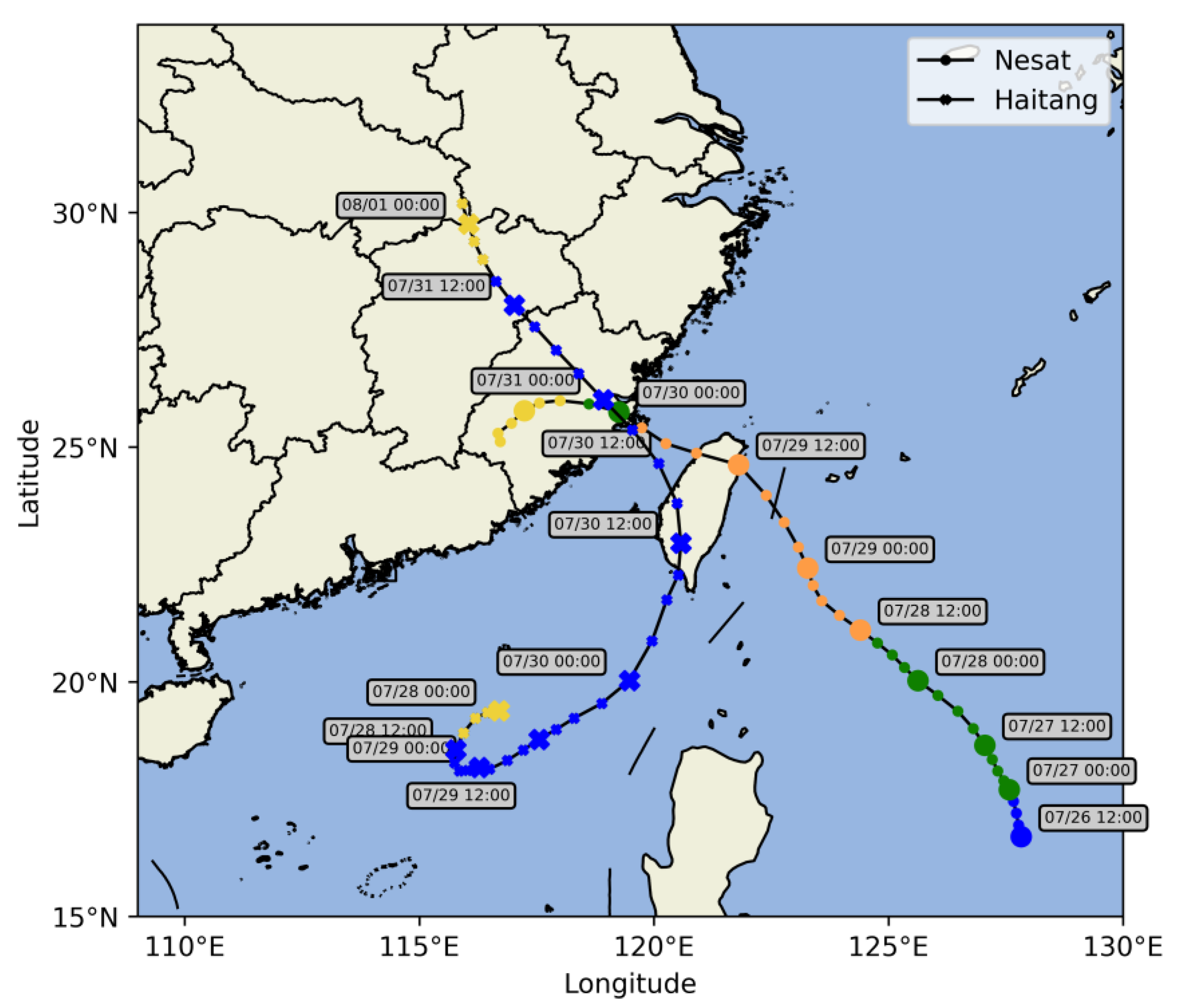
2. Overview of the Binary Typhoons

Nesat originated in the east of the Philippines over the Western North Pacific (WNP) at 0300 UTC on 26 July 2017. After 27 July, Nesat moved west–northwestward at a speed of 15~20 km/h while gradually intensifying. Nesat made its first landfall in northeastern Taiwan at 1200 UTC on 29 July and then for the second time, near Fuqing, Fujian Province, on China’s east coast 10 h later, with the central sea level pressure (SLP) of 975 hPa and maximum surface wind speed (MSW) of 33 m/s. Moving into 30 July, Nesat continued to weaken.
Haitang was formed as a tropical depression on 28 July 2017 over the north of the South China Sea. It became a tropical storm and passed Taiwan Island on 30 July and made a second landfall close to Fuqing at 1900 UTC on 30 July, with a minimum SLP of 990 hPa and a maximum surface wind speed of 18 m/s. After landing, Haitang swallowed up the residual circulation of Nesat and then began weakening steadily as a result of land interaction. The solid lines in Figure 1. show the track of these binary typhoons in 2017.

3. Data, Methodology, and Experiments

3.1. AMDAR Observations and Other Datasets

3.1.1. AMDAR Observations

The AMDAR observations used in this study are provided by China Meteorological Administration (CMA), covering the whole of mainland China spatially (15–60° N, 70–140° E) and vertically between 150 and 700 hPa. The datasets have a time resolution of 3 h from 0000 UTC on 1 July 2017 to 1800 UTC on 31 July 2017 and contain a total of 697,799 pieces of data in this spatial–temporal domain. The variables included in the datasets are time, latitude, longitude, pressure level, temperature, and horizontal wind speed. Figure 2 shows the spatial and temporal distributions of the AMDAR observations, while the frequency distributions of temperature and horizontal wind speed are displayed in Figure 3. In general, the deviation of background (B) and observation (O) is used as a basis for evaluating the quality of the data [17]. Therefore, the frequency distribution in Figure 3 is plotted using the values of the Observation Minus Background (OMB). Further details about the background are provided in Section 3.3.
AMDAR data are mainly distributed along the routes to and from most cities in central and eastern China. In terms of temporal distribution, the AMDAR observations are mainly concentrated between 0300 UTC and 1500 UTC. Most of the data are below the pressure level of 400 hPa, accounting for about 60% of the total data.

3.1.2. Reference Data

In this research, the fifth-generation reanalysis dataset (ERA5) issued by the European Centre for Medium-Range Weather Forecasts (ECMWF) was used to analyze the synoptic environment and verify the forecast results [26]. ERA5 is a global climate reanalysis providing many atmospheric and oceanic parameters (e.g., temperature, pressure, wind, and specific humidity) hourly, with a high spatial resolution (horizontal resolution 0.25° × 0.25° and vertical resolution of 37 pressure levels covered from 1000 hPa to 1 hPa) in GRIB and NetCDF format.
For the location and intensity of TC, we used the International Best Track Archive from Climate Stewardship (IBTrACS) as contrasting information for Nesat and Haitang after the NWP [27,28]. The IBTrACS data were collected from agencies in every ocean basin and processed by the IBTrACS group at the NOAA National Centers for Environmental Information (NCEI), providing the location and intensity (center latitude–longitude, central pressure, maximum sustained wind speed, etc.) of global TCs at least every 6 h.
To evaluate the simulated precipitation that is run by the WRF model, the international Global Precipitation Measurement (GPM) data were applied as a reference [29]. Since its launch in February 2014, GPM has provided a new generation of observations of rainfall and snowfall based on a constellation of satellites deployed by the National Aeronautics and Space Administration (NASA) and Japan Aerospace Exploration Agency (JAXA). The GPM dataset we used has a spatial resolution of 0.1° × 0.1° and a high temporal resolution of 30 min, with a spatial coverage from 60° S to 60° N.

3.2. Introduction of the Two Quality Control Schemes

MCD and OCSVM were used for quality control. Generally, the differences between backgrounds (B) and observations (O) are calculated as the basis for evaluating the quality of the data (OMB). In this study, the deviation of AMDAR data and the GFS field (which was interpolated into the AMDAR locations for comparison) was calculated as the OMB datasets.

3.2.1. MCD

The MCD principle can be formulated as follows [20,30]: Take an n × p data matrix X = ( x 1 , , x n ) , with the i th observation x i = ( x i 1 , , x i p ) R n , i = 1 , , n , so n stands for the number of objects and p for the number of variables. For AMDAR, three variables were chosen; they are u-wind, v-wind, and temperature. So, p = 3 . The Mahalanobis distance in the sample space is defined as follows:
M D x i = ( x i x ¯ ) T S 1 ( x i x ¯ ) ,
where x ¯ is the mean vector of x and S is the covariance matrix of the sample data. It is obvious that using Mahalanobis distance as the criteria for the quality control procedure will be easily influenced by the outliers, because x ¯ is the average of all the samples. In order to increase the robustness of the discrimination, we introduce MCD here. Equation (1) can be written as follows:
R D x i = ( x i μ ¯ M C D ) T Σ ^ M C D 1 ( x i μ ¯ M C D ) ,
where μ ¯ M C D and Σ ^ M C D are the origin point of the sample space and the covariance determinant estimated by MCD, respectively. The main idea of MCD can be shown as follows:
Find a subset H M C D consisting of h observations from X n × p , which keeps the lowest covariance in all the subsets of size h . Therefore, the mean vector μ ¯ M C D of H M C D is chosen as the origin point:
μ ¯ M C D = 1 h i H M C D x i ,
The new covariance matrix is as follows:
Σ ^ M C D = κ M C D ( h , n , p ) h 1 i H M C D ( x i μ ¯ M C D ) ( x i μ ¯ M C D ) T ,
where constant κ M C D ( h , n , p ) is a consistency factor. And for the representativeness, the constraint for the size of H M C D is as follows:
[ ( n + p + 1 ) ] h n ,
Usually, h > p ; it can also be written as
h [ ( n + p + 1 ) / 2 ] ,
In summary, Equation (2), as the discriminant function of MCD, considers a sample as an outlier when the sample’s distance exceeds a certain range.

3.2.2. One Class SVM

The main problem is to discriminate whether a data point x i is an outlier or not, which can be formulated as follows [31]:
f x i = + 1 , i f     x i S 1 , i f     x i S ¯   ,
where S and S ¯ represent the non-outlier and outlier space, respectively.
For the n × p data matrix X = ( x 1 , , x n ) , x i R n , where R n represents the original input space. Let o and R be the original and the radius of the hyper-sphere, respectively. In order to avoid over-fitting, some samples are allowed to be outside the hyper-sphere, so the relaxation variable ξ i is used to obtain the following restriction:
x i o x i o T R 2 + ξ i ,
where ξ i 0 . To minimalize R and ξ i , Equation (2) can be written as follows:
f R , o , ξ i = R 2 + c i ξ i ,
Obviously, it is not a linearly separable problem. Here, we use an algorithm Φ , letting Φ : R n H be a kernel map which transforms the original input space R n into a high-dimensional feature space H . In this study, we choose the Gaussian kernel function as Φ , which will be introduced later. The main idea becomes finding the hyperplane that separates the mapped vectors with maximum margin. In one class SVM, we solve the following quadratic program [32]:
min 1 2 w 2 + 1 ϑ n i = 1 l ξ i ρ Subject   to   ω T Φ x i ρ ξ i   , ξ i 0
where w represents the slope of the hyperplanes in H . Different from Equation (2), the hyperplanes in feature space can be written as follows:
w · x + b = 0 ,
b is a constant, and ϑ ( 0,1 ] is an upper bound on the fraction of training errors and a lower bound of the fraction of support vectors, i.e., a parameter that controls the trade-off between maximizing the distance from the origin and containing most of the data in the region created by the hyperplane and corresponds to the ratio of outliers in the sample dataset. Usually, Equation (4) is written as a dual problem as follows:
min α 1 2 α T Q α , Subject   to   0 α i 1 ϑ n , i = 1 , , n , e T α = 1
where e = [ 1 , , n ] T is the unit vector. Using Q representing the kernel function, which can be written as follows:
Q i j = K x i , x j = Φ x i T Φ x j .
Then, the decision function
f x = s g n i = 1 n α i K x i , x ρ .
The Gaussian kernel function we used is
K x i , x j = e | | x x | | 2 2 σ 2 .

3.3. Numerical Model and Data Assimilation System

The Gridpoint Statistical Interpolation system version 3.7 (GSIv3.7) from NCEP [33] is employed to assimilate the AMDAR data by using the three-dimensional variational (3DVAR) scheme. The DA procedure is valid at 1200 UTC on 28 July 2017. The background of the analysis and the lateral boundaries for NWP are the forecast initiated from the NCEP operational GFS 0.25° × 0.25° analysis at 0000 UTC on 28 July 2017 with a 3 h time interval. For the forecasting of Nesat and Haitang, the Advanced Research version of the Weather Research and Forecasting model (WRF-ARW), version 4.0.2 [34], is chosen with the following physical schemes: the new Thompson scheme [35] for the microphysics; the new version of the Rapid Radiative Transfer Model (RRTMG) [36] for longwave and shortwave radiation; the Tiedtke scheme [37] for cumulus parameterization; the Mellor–Yamada–Janjic scheme [38] for planetary boundary layer process; and the Noah Land Surface Model [39] for land surface. As shown in Figure 4, the domain covers part of the western Pacific Ocean and the east coast of China, consisting of 500 × 300 grid points with a 12 km horizontal grid spacing and 32 vertical levels.

3.4. Experimental Design

To investigate the effects of different QC procedures on AMDAR analyses and binary typhoon forecasting, four experiments were conducted, including a control experiment (EXP-CNTL) and three AMDAR assimilation experiments that used different quality AMDAR observations in the assimilation system (raw, after-mcd, and after-svm, respectively). The experimental design is presented in Table 1.
The control experiment (EXP-CNTL) was just a 72 h simulation run by WRF, which ranged from 12:00 UTC on 28 July 2017 to 12:00 UTC on 31 July 2017, without assimilating any AMDAR data. In the other experiments, AMDAR data of varying quality were assimilated at 12:00 UTC on 28 July 2017. Each of these experiments also extended over a 72 h simulation period. The simulation hours covered the landfall and post-landfall periods of Nesat and Haitang (Figure 1), during which the binary typhoons made rainfall and combined. The AMDAR assimilation experiments were divided into three cases: EXP-RAW, EXP-MCD, and EXP-SVM. EXP-RAW assimilated all the AMDAR data to demonstrate whether the assimilation of AMDAR improves the analysis, while the EXP-MCD and EXP-SVM aimed to show if the two QC methods (MCD and OC-SVM, respectively) can make a better effect.

4. Results

4.1. Quality Change in AMDAR Data

To evaluate the impact of the MCD- and OCSVM- QC schemes on the quality of AMDAR data, the density distribution of AMDAR data was analyzed before and after the implementation of the two QC schemes. Meanwhile, the root mean square error (RMSE) was calculated for AMDAR in different processing stages (AMDAR-all, after QC-MCD, and after QC-SVM), with ERA5 reanalysis used as a reference.
According to Figure 5, both the MCD and OCSVM schemes can reduce the kurtosis and skewness of the AMDAR data. The MCD method reduces more, and the processed data conform more to the Gaussian distribution compared with the AMDAR-RAW and the data processed using the after-SVM method. This is consistent with the principles of the two quality control schemes.
Figure 5 shows that the use of both MCD and OCSVM as QC methods has a similar impact on data quality. Under 200 hPa, the RMSE of u-wind and v-wind decreased by about 0.4 m/s after QC. There was no significant change in the RMSE of AMDAR temperature before and after quality control, according to Figure 6.

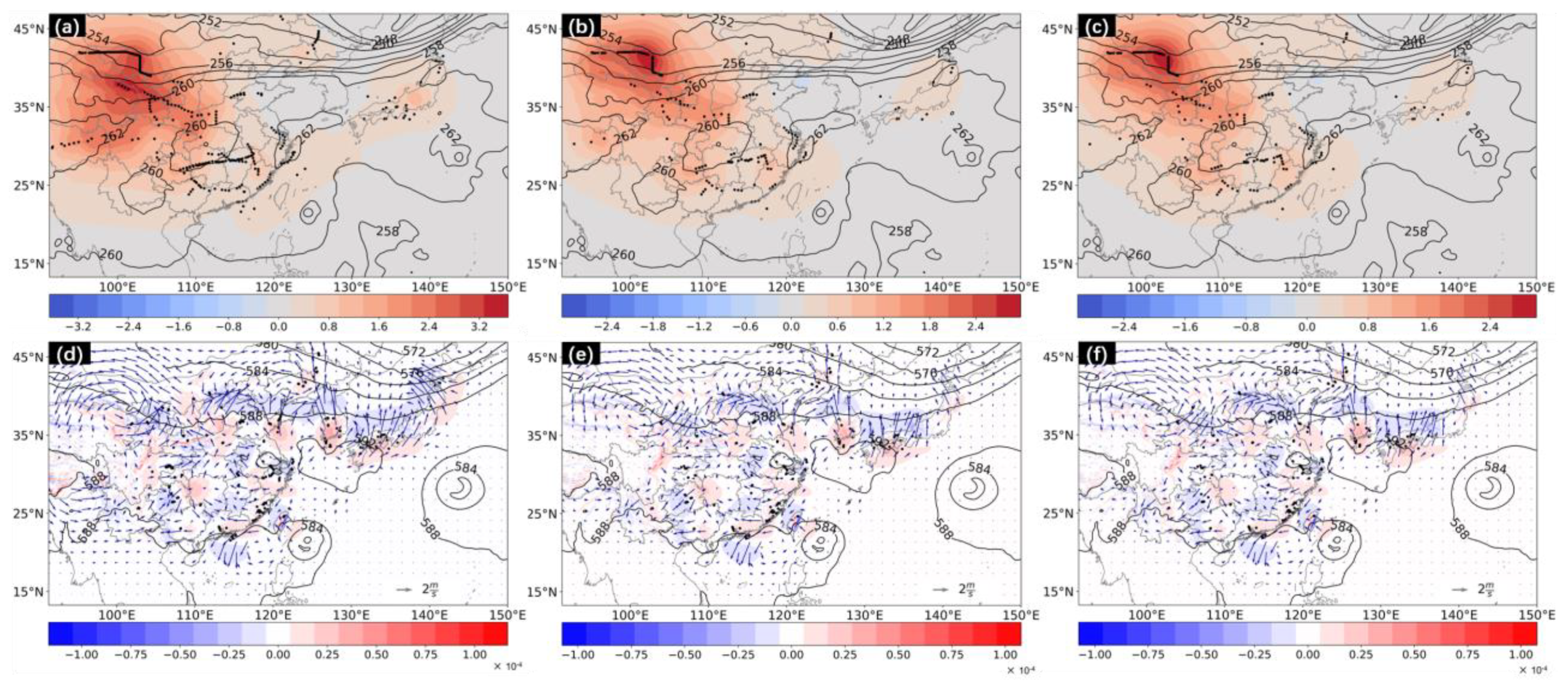
4.2. Analysis Results with AMDAR Data Assimilation

Figure 7 and Figure 8 show the analysis increments of temperature and horizontal wind at the middle and upper levels from EXP-RAW, EXP-MCD, and EXP-SVM at 1200 UTC on 28 July 2017. In order to clarify the contribution of AMDAR wind observations to the domain, the divergency increments were also demonstrated. According to the temperature increment field at 200 hPa in EXP-RAW (Figure 7a), the assimilation of AMDAR observations generated a large band-like warmer area extending over the subtropical high, with an increase of nearly 1 °C, and the center of the maximum increment is pretty closely collocated with the location of the observations on the right side of 120° E. While after QC, most of the observations over the ocean were filtered out, resulting in the original positive temperature increment zone being split into two warm centers. In the EXP-MCD experiment, the warmer area on the northeast side is stronger, while in the EXP-SVM experiment, the one on the southwest side is stronger. For the EXP-CNTL experiment, a negative divergence increment appeared over the center of Nesat, which was caused by the increment of southerly wind. However, this increment was filtered out in both QC methods, as shown in Figure 7e. The wind vector increments also show an anticyclone circulation in the northwest of mainland China. Over the area of the subtropical high, there is a southerly wind increment leading to a mass outflow.
In terms of the analysis increments at middle levels, the three experiments showed strong agreement on the distribution patterns of both temperature and horizontal wind, with the only difference being the reduction in the magnitude of increments after QC (Figure 8). It is evident that the AMDAR observations provided a warmer environment than the GFS at 400 hPa over the first island chain and mainland China. The largest positive temperature increments (about 3.4 °C for EXP-CNTL and 3.0 °C for EXP-MCD and EXP-SVM) were observed in northwest China, where a large cyclonic circulation increment overlapped at 500 hPa according to the wind field. Additionally, a northward component of wind increments was observed over the area of the binary typhoons.

4.3. Forecasting Results

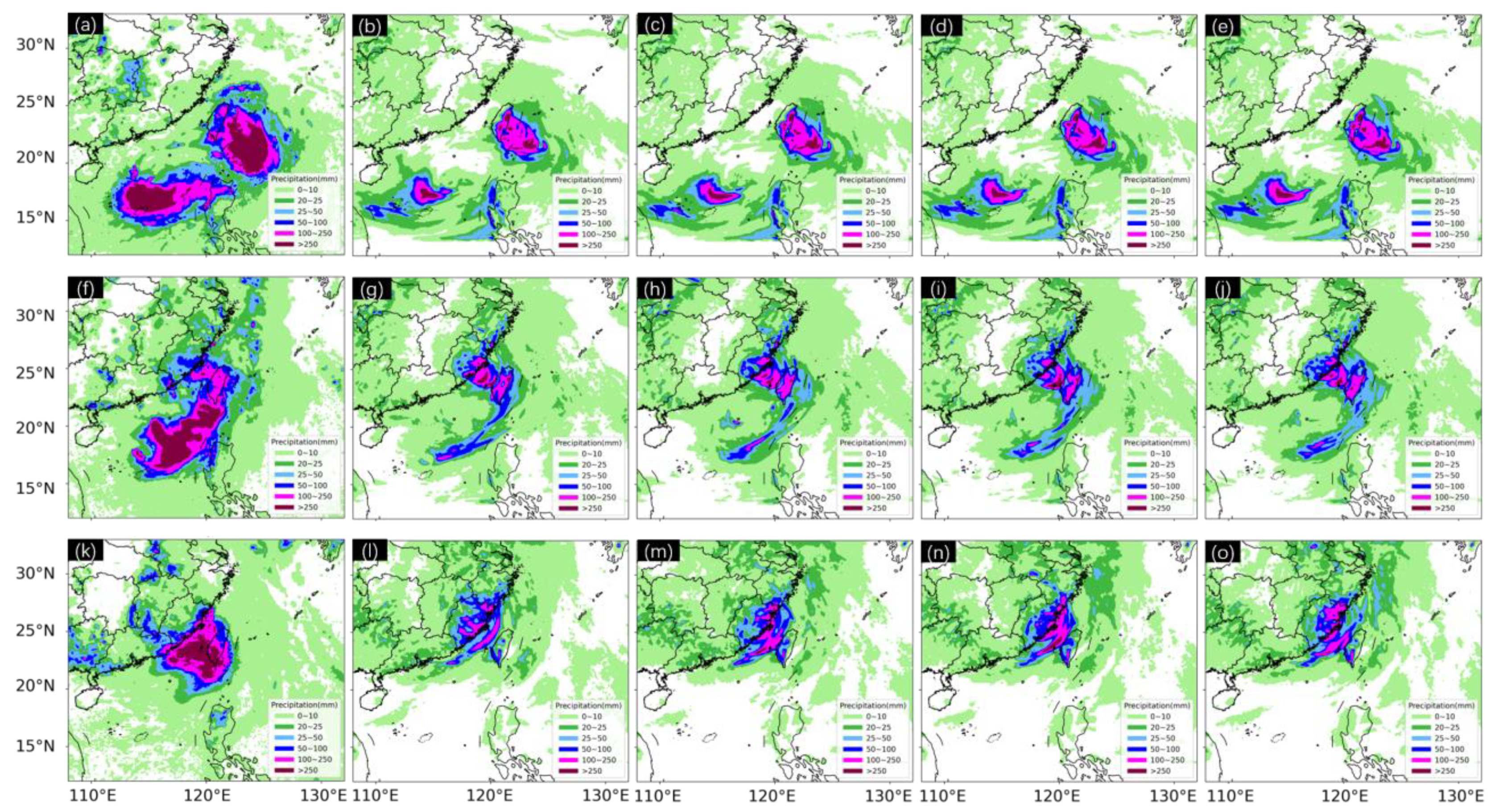
4.3.1. Precipitation Forecasts

Figure 9 shows the precipitation fields accumulated every 24 h for different periods during and after the landfall from CNTL, EXP-RAW, EXP-MCD, and EXP-SVM, respectively, from 12:00 UTC on 28–31 July, as compared to GPM rainfall data (first column of Figure 9). It is obvious that the four WRF experiments slightly underpredicted the range of precipitation. During the first 24 h of the forecast period (12:00 UTC on 28 to 29, Figure 9a–e), GPM showed two heavy precipitation regions in the South China Sea. The northeastern one was caused by Nesat passing through Taiwan Island, and the other one on the ocean surface was caused by Haitang. Though, in general, the precipitation ranges of all four experiments were similar and significantly smaller than those of GPM, the magnitude of the precipitation on the land surface of Taiwan Province was on the high side. In the next 24 h (Figure 9f–j), Nesat and Haitang made landfall in Fuqing, Fujian Province in sequence and then merged together under the Fujiwara effect. GPM showed two maximum centers over the east of Guangdong Province and central Fujian. It is evident that the Nesat circulation in the GFS background is more north, causing the northward rainfall area in Fujian and Zhejiang provinces; this may be due to its northward track bias. Note that the magnitude of the heavy precipitation center in Fujian from EXP-CNTL was overpredicted, with a maximum of about 258.9 mm, much larger than 97.8 mm in GPM. The overprediction of the rainfall in Fujian was lightened to a certain extent by the assimilation of AMDAR data, but still larger than that of the GPM. By contrast, EXP-SVM generated a smaller maximum precipitation of about 171.0 mm in Fujian than the 189.7 mm and 218.6 mm from EXP-RAW and EXP-MCD, respectively. The precipitation shown in Figure 9k–o is conducted to the circulation merged by Nesat and Haitang. GPM shows that the precipitation center was mainly at the sea, and the rainfall on the mainland mainly occurred in the coastal areas of Fujian. The precipitation center of the four experiments was significantly northward, and the precipitation area over the land was larger than the actual situation, while the precipitation in Taiwan was underpredicted. With the assimilation of AMDAR, the rainfall in the south of Fujian province predicted by EXP-RAW is obviously reduced, and the range of EXP-MCD is closer to that of the GPM than that of EXP-SVM.
To quantitatively evaluate the precipitation forecast, threat scores (TS) were calculated based on the accumulated precipitation every 24 h from the four experiments against the GPM precipitation data from 1200 UTC on 28–31 July (as shown in Figure 10, consistent with Figure 9) [40]. For the first 48 h, the ability of precipitation forecast decreased at all thresholds compared with the EXP-CNTL when AMDAR was joint in the assimilation procedure. This situation can be alleviated by QC, which even enhanced the prediction capabilities in some cases (e.g., EXP-SVM at 25 mm threshold in Figure 10c and EXP-MCD and EXP-SVM at 10 mm and 25 mm thresholds in Figure 10a,b). But from 48 to 72 h, EXP-RAW performed better in the moderate to heavy rainfall (≥ 25 mm) range, and the use of SVM as a QC method improved the advantage of assimilating AMDAR data during this stage. However, EXP-MCD had a lower score during this period, but had the highest score among the four experiments at the 100 mm threshold. Overall, the assimilation of AMDAR data has negative impacts on the precipitation forecast in the short-term period, but has positive impacts on the long-term forecast. The SVM scheme has a positive effect on the forecast of moderate precipitation (10~25 mm), while the MCD scheme makes a significant contribution to the long-term heavy rainfall forecast.

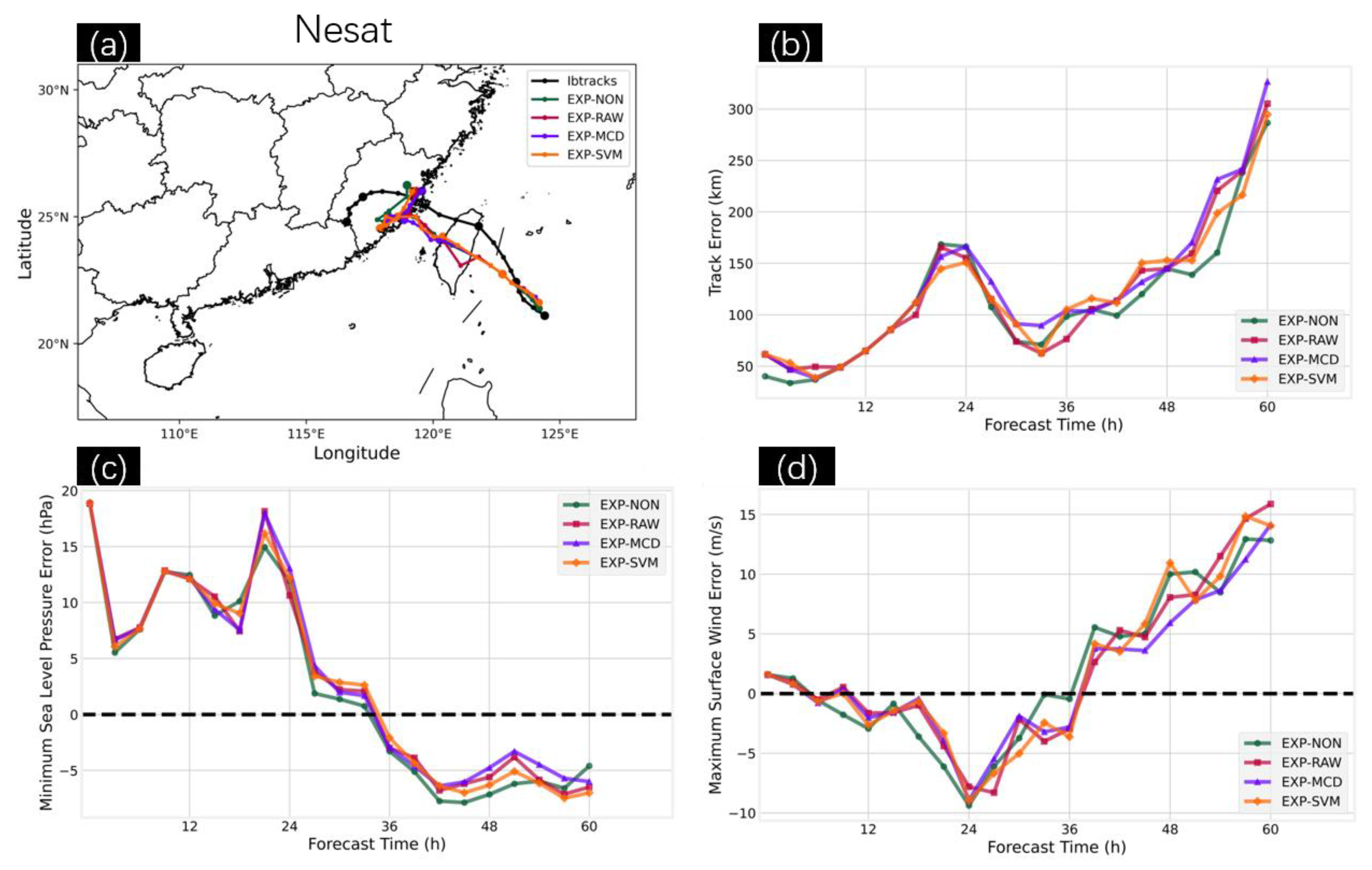
4.3.2. Track and Intensity Predictions

Due to the rapid dissipation of the typhoon and the challenges in capturing its inner-land circulation structure in the four experiments, we focused our statistical analysis on the first 60 h of track and intensity forecasts for Typhoon Nesat. Similarly, for Typhoon Haitang, we considered the first 54 h of forecasts. Figure 11 shows the 60 h track and intensity forecasts of Nesat, initialized at 1200 UTC on 28 July 2017; the black lines represent the best track from IBTrACS, which is used as the reference. The track of Nesat simulated by the GFS field was further south than that of IBTrACS, resulting in all four WRF experiments failing to meet the expectations in predicting the two landfall points of the typhoon. The northwestward movement was observed to turn northeastward along the coast after Nesat’s second landfall, which is inconsistent with the deep inland path shown in IBTrACS. According to EXP-RAW, assimilating all AMDAR data caused a significant southward deviation when Nesat passed over Taiwan, and the deviation was eliminated in both EXP-MCD and EXP-SVM after QC was applied. EXP-SVM had a slightly lower track error in the first 24 h, while the EXP-CNTL performed better after 36 h. In terms of Nesat’s intensity forecast, the GFS model predicted the storm to be weaker in the first 36 h (with higher SLP and lower MWS), but then stronger after 36 h. Assimilating AMDAR data helped correct this bias to a certain extent. Overall, the EXP-MCD experiment, which used MCD as the QC scheme, had a better performance in forecasting the intensity of Nesat than the other three experiments.
Figure 12 displays the 54 h track and intensity forecasts of Haitang, which were initialized at 1200 UTC on 28 July 2017. Based on the results from EXP-CNTL shown in Figure 12a, it can be seen that the track for Haitang simulated by the GFS was significantly further south than that in IBTrACS. Additionally, the circulation structure of Haitang dissipated at 0600 UTC on 30 July 2017. However, the assimilation of AMDAR data caused Haitang to have a longer maintenance, resulting in Typhoon Haitang making landfall at 1800 UTC on 30 July and then being absorbed by Nesat. Assimilation AMDAR in the initial field also caused a northward deviation in track forecasting of the three assimilation experiments (EXP-RAW, EXP-MCD, and EXP-SVM) when compared with the IBTrACS. None of the four experiments made an accurate forecast on both the landfall point and the path passing through Taiwan. According to the track error forecasts shown in Figure 12b, it is evident that the first 12 h exhibited a significant track error, which was attributed to the slow movement of Haitang predicted in the GFS field. EXP-RAW performed better in the early stages, while EXP-MCD performed better later on. In terms of the entire simulation period, the track error of EXP-SVM is the smallest (120 km on average, compared to 121 km and 126 km for EXP-RAW and EXP-MCD, respectively. EXP-CNTL was not included in the comparison due to insufficient forecast time). As for intensity forecasting, the three assimilated experiments exhibited different strengths and weaknesses at different times, with EXP-MCD showing smaller intensity forecast errors, particularly during the later stages of the simulation.

5. Conclusions and Discussion

In this study, two quality control (QC) methods, MCD and OCSVM, were applied to assess the impact of AMDAR data on track and intensity forecasts for the binary typhoons Nesat and Haitang (2017), utilizing the GSI DA system and regional WRF model. The results demonstrate that the assimilation of AMDAR data can significantly impact the precipitation and the accuracy of track and intensity forecasts of typhoons, especially when combined with appropriate QC methods. In particular, it helped correct the southward deviation of Nesat’s track when it passed over Taiwan and resulted in a longer maintenance of Haitang, which led to a more accurate forecast of its landfall time and resulted in more precipitation. The effectiveness of different QC methods on the assimilation experiments varied. The MCD method was found to be the most effective in improving the intensity forecast of Nesat, while the OCSVM method had a slightly better performance in the early stages of the track forecast. In general, the performance of the three assimilation experiments was similar, with each having its strengths and weaknesses.
This study demonstrated that assimilating AMDAR data could improve the accuracy of typhoon forecasts to some extent, but the QC methods used were also crucial in minimizing the impact of errors in the observations. Note that our conclusions are obtained from the analysis of one binary typhoon case. Consequently, the generalizability of these conclusions may be limited. Future investigations should encompass a series of experiments to quantitatively assess the influence of the two QC methods on AMDAR assimilation and their implications for typhoon prediction. From the outcomes of our experiments, it is evident that there still exists notable deviation in typhoon track prediction. This discrepancy can be attributed to factors such as the selection of background fields and the configuration of the physical schemes within the model. Going forward, we are committed to refining our experimental setups to better align with operational requirements. This includes the exploration of techniques such as four-dimensional variational data assimilation (4D-Var) and the incorporation of additional observational data. These endeavors aim to further investigate suitable QC strategies for AMDAR data in the context of typhoon forecasting.

Author Contributions

Conceptualization, Y.Z.; methodology, Y.Z. and J.L.; software, Y.Z. and D.W.; validation, J.H., J.F. and Q.T.; formal analysis, J.L.; investigation, J.L.; resources, Y.Z. and J.K.; data curation, J.K.; writing—original draft preparation, J.L.; writing—review and editing, Y.Z.; visualization, S.C., D.S. and J.H.; supervision, Y.Z.; project administration, Y.Z.; funding acquisition, Y.Z. All authors have read and agreed to the published version of the manuscript.

Funding

This study was jointly supported by Guangdong Ocean University Scientific Research Startup Fund (R20021), Guangdong Province Natural Science Foundation Youth Science Fund (2021A1515110944), and the Foundation of Meteorological Observation Centre of CMA for Young Scientists (Grant No. MOCQN202103).

Institutional Review Board Statement

Not applicable.

Informed Consent Statement

Informed consent was obtained from all subjects involved in the study.

Data Availability Statement

Data were obtained from the Meteorological Observation Centre of CMA and are available from the authors with the permission of the Meteorological Observation Centre of CMA.

Acknowledgments

I would like to express my sincere gratitude to the following individuals for their valuable contributions to this research project. Zhang provided invaluable guidance and mentorship throughout the entire process, from the initial conceptualization to the final revision. I am also grateful to my research participants in the ‘WE-HATE-NWP’ group for their willingness to share their insights and experiences. Finally, I would like to thank my family and friends for their unwavering support and encouragement throughout this journey. We also want to express our sincere gratitude for the time and effort invested by all the reviewers and editors in evaluating our work. We truly appreciate the constructive criticism and insightful suggestions that have been provided, which have undoubtedly contributed to the enhancement of the manuscript.

Conflicts of Interest

The authors declare no conflict of interest.

References

  1. Petersen, R.A.; Cronce, L.; Mamrosh, R.; Baker, R.; Pauley, P. On the Impact and Future Benefits of AMDAR Observations in Operational Forecasting: Part II: Water Vapor Observations. Bull. Am. Meteorol. Soc. 2016, 97, 2117–2133. [Google Scholar] [CrossRef]
  2. WMO. Aircraft Meteorological Data Relay (AMDAR) Reference Manual; Secretariat of the World Meteorological Organization: Geneva, Switzerland, 2003; ISBN 978-92-63-10958-3. [Google Scholar]
  3. WMO. Guide to Aircraft-Based Observations (WMO-No. 1200), 2017th ed.; WMO: Geneva, Switzerland, 2017; ISBN 978-92-63-11200-2. [Google Scholar]
  4. Ballish, B.A.; Kumar, V.K. Systematic Differences in Aircraft and Radiosonde Temperatures: Implications for NWP and Climate Studies. Bull. Am. Meteorol. Soc. 2008, 89, 1689–1708. [Google Scholar] [CrossRef]
  5. Cardinali, C.; Isaksen, L.; Andersson, E. Use and Impact of Automated Aircraft Data in a Global 4DVAR Data Assimilation System. Mon. Weather Rev. 2003, 131, 1865–1877. [Google Scholar] [CrossRef]
  6. Petersen, R.A. On the Impact and Benefits of AMDAR Observations in Operational Forecasting—Part I: A Review of the Impact of Automated Aircraft Wind and Temperature Reports. Bull. Am. Meteorol. Soc. 2016, 97, 585–602. [Google Scholar] [CrossRef]
  7. Zhong, J.Q.; Chen, M.; Fan, S.Y. Assimilation Application of AMDAR Data to the Operational NWP System of Beijing. J. Appl. Meteorol. Sci. 2010, 21, 19–28. [Google Scholar]
  8. Petersen, R.A.; Cronce, L.; Mamrosh, R.; Baker, R. Impact and Benefits of AMDAR Temperature, Wind, and Moisture Observations in Operational Weather Forecasting; WMO: Geneva, Switzerland, 2015; p. 93. [Google Scholar]
  9. Hoover, B.T.; Velden, C.S.; Langland, R.H. Adjoint-Based Analysis of Observational Impact on Tropical Cyclone Forecasts. In Proceedings of the 31st Conference on Hurricanes and Tropical Meteorology, San Diego, CA, USA, 31 March–4 April 2014. [Google Scholar]
  10. Rui-wen, W.; Wei, H.; Wei-hong, T.; Jian-dong, G. Blacklist Design of AMDAR Temperature Data and Their Application in the CMA-GFS. JTM 2021, 27, 368–377. [Google Scholar] [CrossRef]
  11. Chunyan, S.; Shijun, L.; Sudan, F. Effect Study of Different AMDAR Data Assimilation Time Window to Typhoon Yagi. J. Mar. Meteorol. 2021, 41, 11–25. [Google Scholar]
  12. Liao, J.; Wang, H.; Zhou, Z.; Liu, Z.; Jiang, L.; Yuan, F. Integration, Quality Assurance, and Usage of Global Aircraft Observations in CRA. J. Meteorol. Res. 2021, 35, 1–16. [Google Scholar] [CrossRef]
  13. United States National Weather Service Systems Development Office Technique Specification Package 88-21-R2 for Awips-90 Rfp Appendix G Requirements Numbers 2. 1 Quality Control Incoming Data; U.S. Dept. of Commerce National Oceanic and Atmospheric Administration National Weather Service Office of Systems Development: Washington, DC, USA, 1994.
  14. Sako, H. Assimilation of Aircraft Temperature Data in the JMA Global 4D-Var Data Assimilation System. CAS/JSC WGNE Res. Activ. Atmos. Ocean. Model. 2010, 40, 33–34. [Google Scholar]
  15. James, E.P.; Benjamin, S.G.; Jamison, B.D. Commercial-Aircraft-Based Observations for NWP: Global Coverage, Data Impacts, and COVID-19. J. Appl. Meteorol. Climatol. 2020, 59, 1809–1825. [Google Scholar] [CrossRef]
  16. Dahoui, M.; Bormann, N.; Isaksen, L. Automatic Checking of Observations at ECMWF; ECMWF: Reading, UK, 2016. [Google Scholar]
  17. Duan, B.; Zhang, W.; Yang, X.; Dai, H.; Yu, Y. Assimilation of Typhoon Wind Field Retrieved from Scatterometer and SAR Based on the Huber Norm Quality Control. Remote Sens. 2017, 9, 987. [Google Scholar] [CrossRef]
  18. Rousseeuw, P.J. Least Median of Squares Regression. J. Am. Stat. Assoc. 1984, 79, 871–880. [Google Scholar] [CrossRef]
  19. Rousseeuw, P. Multivariate Estimation with High Breakdown Point. In Mathematical Statistics and Applications; Reidel Publishing Company: Dordrecht, The Netherlands, 1985; p. 37. [Google Scholar] [CrossRef]
  20. Hubert, M.; Debruyne, M. Minimum Covariance Determinant. WIREs Comput. Stat. 2010, 2, 36–43. [Google Scholar] [CrossRef]
  21. Rousseeuw, P.J.; Driessen, K.V. A Fast Algorithm for the Minimum Covariance Determinant Estimator. Technometrics 1999, 41, 212–223. [Google Scholar] [CrossRef]
  22. Butler, R.W.; Davies, P.L.; Jhun, M. Asymptotics for the Minimum Covariance Determinant Estimator. Ann. Stat. 1993, 21, 1385–1400. [Google Scholar] [CrossRef]
  23. Cortes, C.; Vapnik, V. Support-Vector Networks. Mach. Learn. 1995, 20, 273–297. [Google Scholar] [CrossRef]
  24. Boswell, D. Introduction to Support Vector Machines; Departement of Computer Science and Engineering University of California San Diego: San Diego, CA, USA, 2002; p. 11. [Google Scholar]
  25. Schölkopf, B.; Platt, J.C.; Shawe-Taylor, J.; Smola, A.J.; Williamson, R.C. Estimating the Support of a High-Dimensional Distribution. Neural Comput. 2001, 13, 1443–1471. [Google Scholar] [CrossRef]
  26. Hersbach, H.; Bell, B.; Berrisford, P.; Hirahara, S.; Horányi, A.; Muñoz-Sabater, J.; Nicolas, J.; Peubey, C.; Radu, R.; Schepers, D.; et al. The ERA5 Global Reanalysis. Q. J. R. Meteorol. Soc. 2020, 146, 1999–2049. [Google Scholar] [CrossRef]
  27. Knapp, K.R.; Kruk, M.C.; Levinson, D.H.; Diamond, H.J.; Neumann, C.J. The International Best Track Archive for Climate Stewardship (IBTrACS): Unifying Tropical Cyclone Data. Bull. Am. Meteorol. Soc. 2010, 91, 363–376. [Google Scholar] [CrossRef]
  28. Knapp, K.R.; Diamond, H.J.; Kossin, J.P.; Kruk, M.C.; Schreck, C.J. International Best Track Archive for Climate Stewardship (IBTrACS) Project, Version 4; NOAA National Centers for Environmental Information: Washington, DC, USA, 2018. [Google Scholar]
  29. Hou, A.Y.; Kakar, R.K.; Neeck, S.; Azarbarzin, A.A.; Kummerow, C.D.; Kojima, M.; Oki, R.; Nakamura, K.; Iguchi, T. The Global Precipitation Measurement Mission. Bull. Am. Meteorol. Soc. 2014, 95, 701–722. [Google Scholar] [CrossRef]
  30. Hubert, M.; Debruyne, M.; Rousseeuw, P.J. Minimum Covariance Determinant and Extensions. WIREs Comput. Stat. 2018, 10, e1421. [Google Scholar] [CrossRef]
  31. Wang, Y.; Wong, J.; Miner, A. Anomaly Intrusion Detection Using One Class SVM. In Proceedings of the Fifth Annual IEEE SMC Information Assurance Workshop, West Point, NY, USA, 10–11 June 2004; pp. 358–364. [Google Scholar]
  32. Chang, C.-C.; Lin, C.-J. LIBSVM: A Library for Support Vector Machines. ACM Trans. Intell. Syst. Technol. 2011, 2, 27. [Google Scholar] [CrossRef]
  33. Hu, M.; Ge, G.; Zhou, C.; Stark, D.; Shao, H.; Newman, K.; Beck, J.; Zhang, X. Grid-Point Statistical Interpolation (GSI) User’s Guide Version 3.7; Development Testbed Center: Boulder, CO, USA, 2018. [Google Scholar]
  34. Skamarock, W.C.; Klemp, J.B.; Dudhia, J.; Gill, D.O.; Liu, Z.; Berner, J.; Wang, W.; Powers, J.G.; Duda, M.G.; Barker, D.M.; et al. A Description of the Advanced Research WRF Model Version 4; UCAR/NCAR: Boulder, CO, USA, 2019; p. 145. [Google Scholar]
  35. Thompson, G.; Field, P.R.; Rasmussen, R.M.; Hall, W.D. Explicit Forecasts of Winter Precipitation Using an Improved Bulk Microphysics Scheme. Part II: Implementation of a New Snow Parameterization. Mon. Weather Rev. 2008, 136, 5095–5115. [Google Scholar] [CrossRef]
  36. Iacono, M.J.; Delamere, J.S.; Mlawer, E.J.; Shephard, M.W.; Clough, S.A.; Collins, W.D. Radiative Forcing by Long-Lived Greenhouse Gases: Calculations with the AER Radiative Transfer Models. J. Geophys. Res. 2008, 113, D13103. [Google Scholar] [CrossRef]
  37. Zhang, C.; Wang, Y.; Hamilton, K. Improved Representation of Boundary Layer Clouds over the Southeast Pacific in ARW-WRF Using a Modified Tiedtke Cumulus Parameterization Scheme. Mon. Weather Rev. 2011, 139, 3489–3513. [Google Scholar] [CrossRef]
  38. Janjić, Z.I. The Step-Mountain Eta Coordinate Model: Further Developments of the Convection, Viscous Sublayer, and Turbulence Closure Schemes. Mon. Weather Rev. 1994, 122, 927–945. [Google Scholar] [CrossRef]
  39. Niu, G.-Y.; Yang, Z.-L.; Mitchell, K.E.; Chen, F.; Ek, M.B.; Barlage, M.; Kumar, A.; Manning, K.; Niyogi, D.; Rosero, E.; et al. The Community Noah Land Surface Model with Multiparameterization Options (Noah-MP): 1. Model Description and Evaluation with Local-Scale Measurements. J. Geophys. Res. 2011, 116, D12109. [Google Scholar] [CrossRef]
  40. Hamill, T.M. Hypothesis Tests for Evaluating Numerical Precipitation Forecasts. Weather Forecast. 1999, 14, 155–167. [Google Scholar] [CrossRef]
Figure 1. Map of the moving paths of Nesat and Haitang in July 2017. Different colors indicate varying typhoon intensities: yellow points represent tropical depression (TD), blue points represent tropical storm (TS), green points represent strong tropical storm (STS), and orange points represent typhoon (TY).
Atmosphere 14 01341 g001
Figure 2. The distribution of AMDAR observations in July 2017. (a) AMDAR observations’ spatial distribution map, where colors represent the pressure levels. (b) Statistics of AMDAR observations over time and altitude.
Atmosphere 14 01341 g002
Figure 3. The density distribution of the (a) u-wind, (b) v-wind, and (c) temperature differences (OMB) in July 2017. The solid lines represent the Gaussian distribution according to the mean values and standard deviations of the differences.
Atmosphere 14 01341 g003
Figure 4. Model domain configuration (black square).
Atmosphere 14 01341 g004
Figure 5. The density distribution of u-wind (the first column), v-wind (the second column), and temperature (the last column) differences (O-B) from 1 to 31 July 2017. The solid lines represent the Gaussian distribution according to the mean values and standard deviations of the differences. (ac) use all the AMDAR data, (df) use the AMDAR data after removing outliers with QC-MCD, (gi) use the AMDAR data after removing outliers with QC-SVM.
Atmosphere 14 01341 g005
Figure 6. RMSE profile of AMDAR data for AMDAR-all (red lines represent all the AMDAR data without moving any outliers), after QC-MCD (yellow lines represent the AMDAR data after removing outliers identified by QC-MCD method), and after QC-SVM (purple lines, represent the AMDAR data after removing outliers identified by QC-SVM method) against ERA-5: (a) u-wind, (b) v-wind, and (c) temperature at 1200 UTC on 28 July 2017.
Atmosphere 14 01341 g006
Figure 7. The analysis increments of ((ac), shaded colors; K) temperature and ((df), arrows; m/s) horizontal wind at 200 hPa after AMDAR assimilation for the experiments EXP-RAW (the first column), EXP-RAW (the second column), and EXP-RAW (the last column) at 00 UTC on 28 July 2017. The black dots show the location of the AMDAR observation. Shaded colors in (df) represent the horizontal divergence increments. Labeled line contours are (ac) temperature (K) and (e,f) geopotential heights (gpm) from GFS backgrounds.
Atmosphere 14 01341 g007
Figure 8. Same as Figure 7, but the pressure level for the ((ac), shaded colors; K) temperatureand ((df), arrows; m/s) horizontal wind increments are 400 hPa and 500 hPa, respectively.
Atmosphere 14 01341 g008
Figure 9. The 24 h accumulated precipitation (mm) according to the GPM (the first column), EXP-CNTL (the second column), EXP-RAW (the third column), EXP-SVM (the fourth column), and EXP-SVM (the last column) valid at 1200 UTC, (ae) 28, (fj) 29, and (ko) 30 July 2017.
Atmosphere 14 01341 g009
Figure 10. The threat scores (TS) for the forecasts of 24 h accumulated precipitation for the 3 days from 1200 UTC on 28–31 July 2017. Subplots (ac) correspond to TS values for the varing forecast intervals: (a) from 1200 UTC on 28 July to 1200 UTC on 29 July, (b) from 1200 UTC on 29 July to 1200 UTC on 30 July, and (c) from 1200 UTC on 30 July to 1200 UTC on 31 July.
Atmosphere 14 01341 g010
Figure 11. Tracks and intensity predictions of Nesat. (a) The best track from IBTrACS (black line) and experiments for EXP-CNTL (green line), EXP-RAW (red line), EXP-MCD (purple line), and EXP-SVM (yellow line). (b) The track errors for experiments against IBTrACS. (c) Same as (b) but for MSLP errors. (d) Same as (b) but for MSW errors.
Atmosphere 14 01341 g011
Figure 12. Same as Figure 11, but for Haitang. (a) The best track from IBTrACS (black line) and experiments for EXP-CNTL (green line), EXP-RAW (red line), EXP-MCD (purple line), and EXP-SVM (yellow line). (b) The track errors for experiments against IBTrACS. (c) Same as (b) but for MSLP errors. (d) Same as (b) but for MSW errors.
Atmosphere 14 01341 g012
Table 1. The setting of all the QC and NWP experiments.
ExperimentDescription
EXP-CNTLNo data assimilation
EXP-RAWAssimilating all the AMDAR data
EXP-MCDAssimilating the AMDAR data after removing outliers identified by QC-MCD method
EXP-SVMAssimilating the AMDAR data after removing outliers identified by OC-SVM method
Disclaimer/Publisher’s Note: The statements, opinions and data contained in all publications are solely those of the individual author(s) and contributor(s) and not of MDPI and/or the editor(s). MDPI and/or the editor(s) disclaim responsibility for any injury to people or property resulting from any ideas, methods, instructions or products referred to in the content.

