


Aerosol Optical Properties and Type Retrieval via Machine Learning and an All-Sky Imager

 , and
, and
Abstract
:1. Introduction
- The application of a supervised learning technique for retrieving AOD at 440, 500, and 674 nm (AOD440 nm, AOD500 nm, and AOD675 nm), Ångström Exponent between 440 and 675 nm (AE440–675 nm), and Fine Mode Fraction at 500 nm (FMF500 nm) using valuable sky information from an ASI;
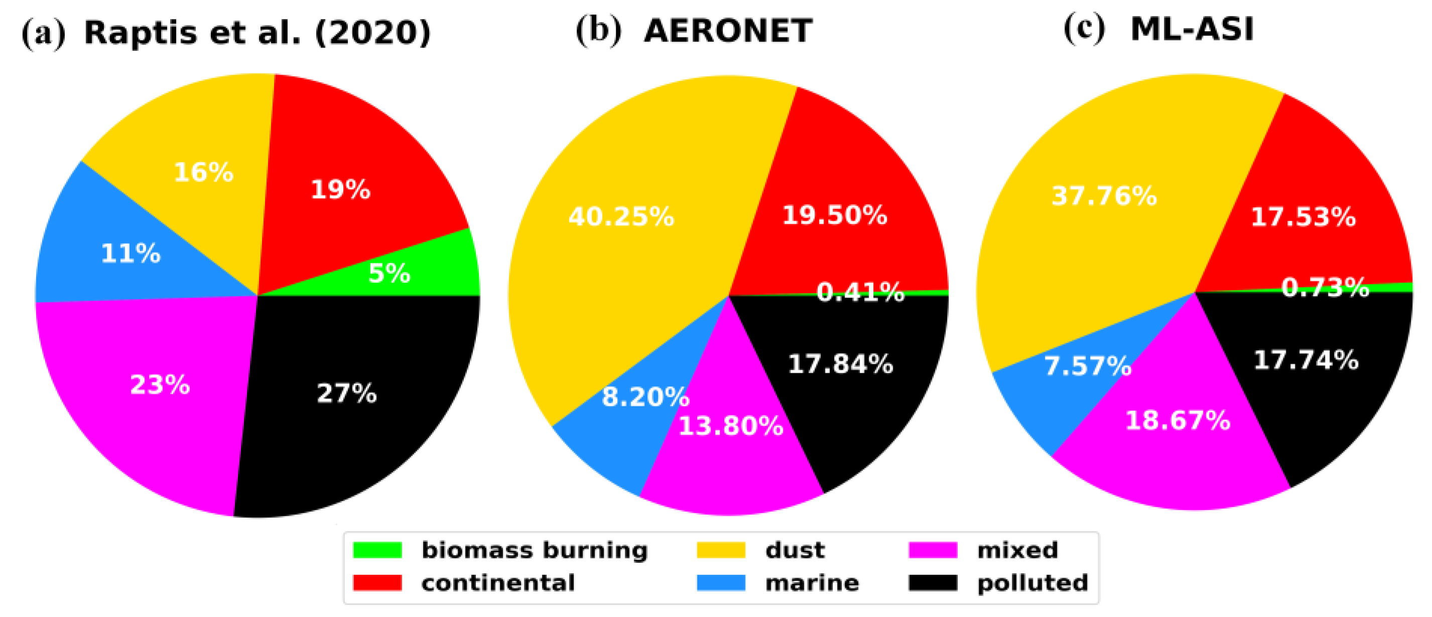
- The efficiency of the results in performing aerosol-type classification.
2. Data
2.1. Measurement Site
2.2. Measuring Instruments
2.2.1. AERONET Station
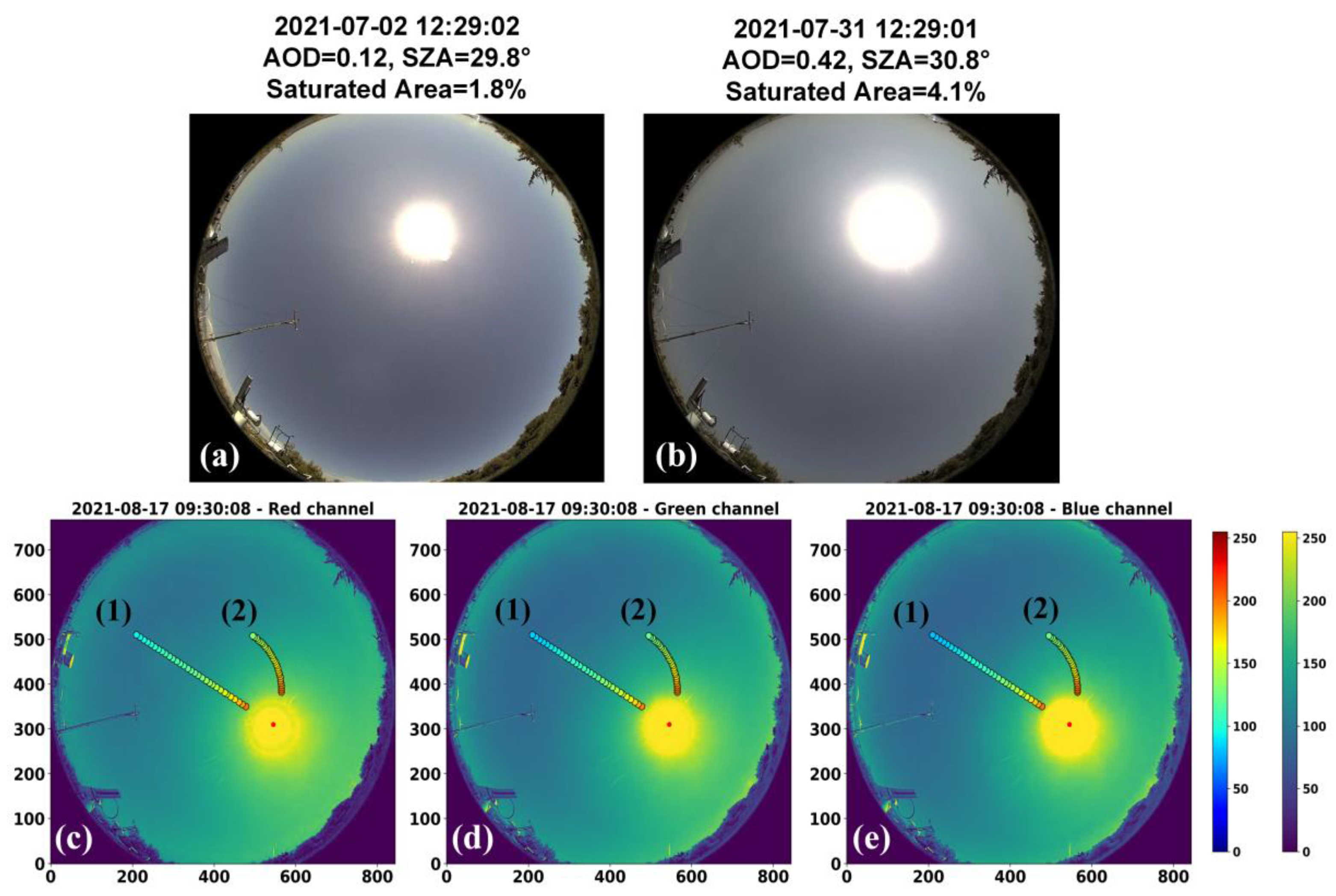
2.2.2. All-Sky Imager
3. Methodology
3.1. Machine Learning Approach
3.2. Validation Metrics
4. Results
4.1. Performance of the Retrieved Aerosol Optical Properties
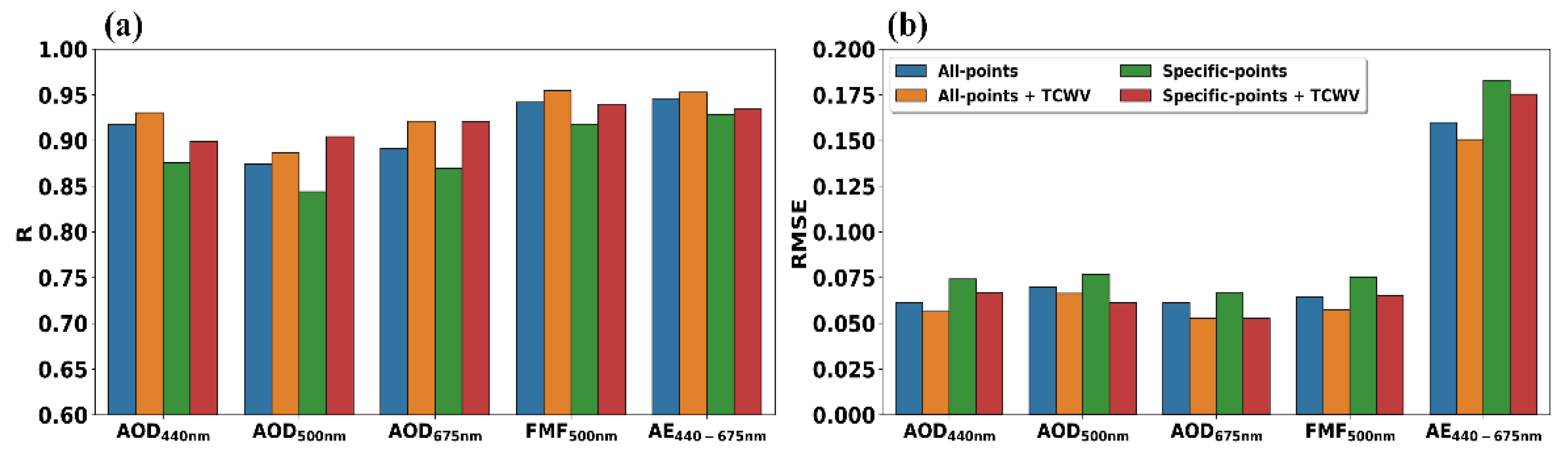
4.1.1. Sensitivity Analysis on Model Input Parameters and ML Application
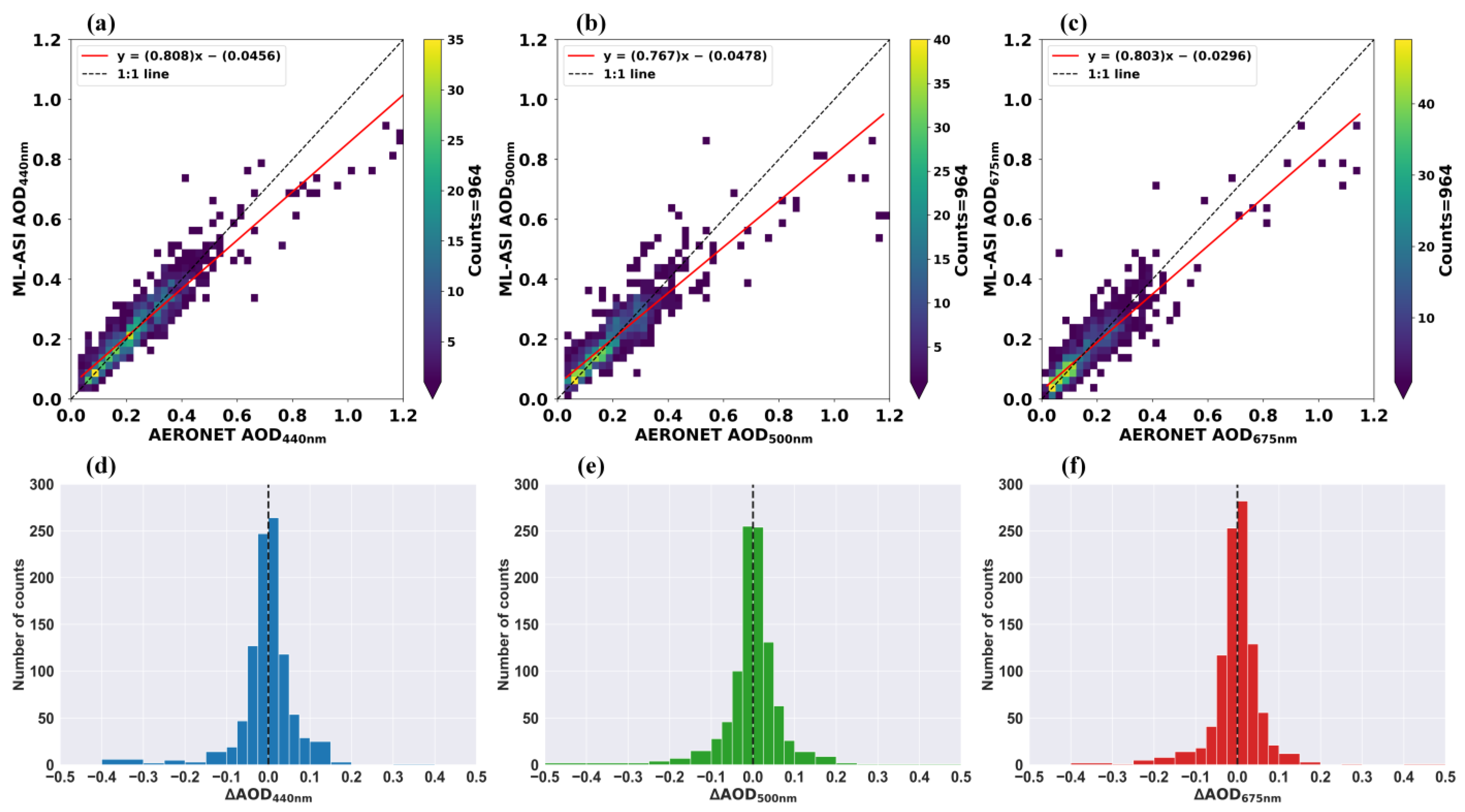
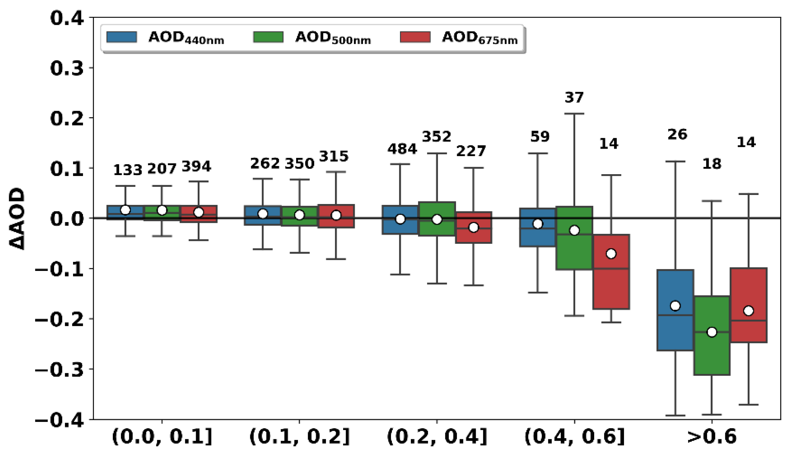
4.1.2. Aerosol Optical Depth Retrieval Performance
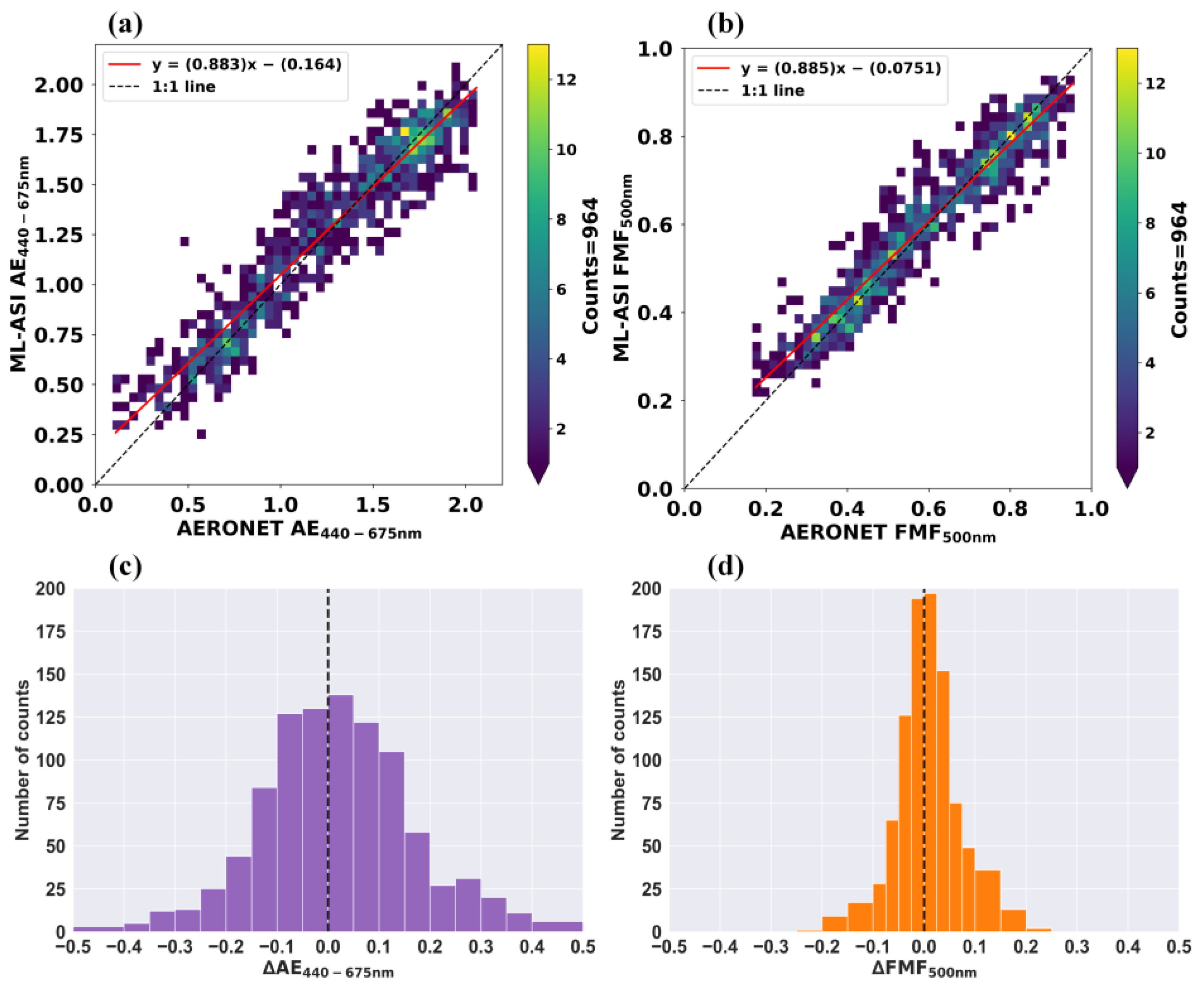
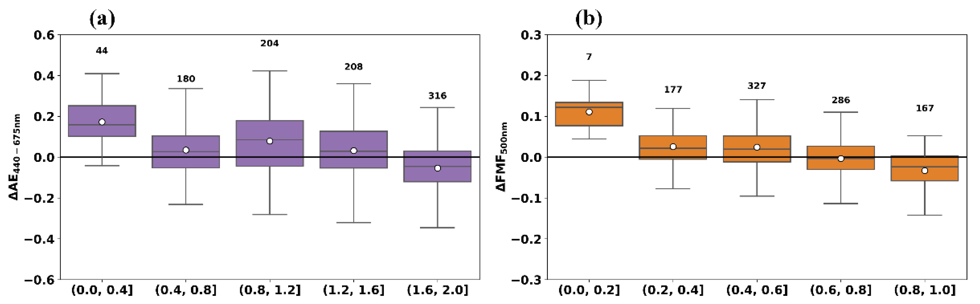
4.1.3. AE440–675 nm and FMF500 nm Retrieval Performance
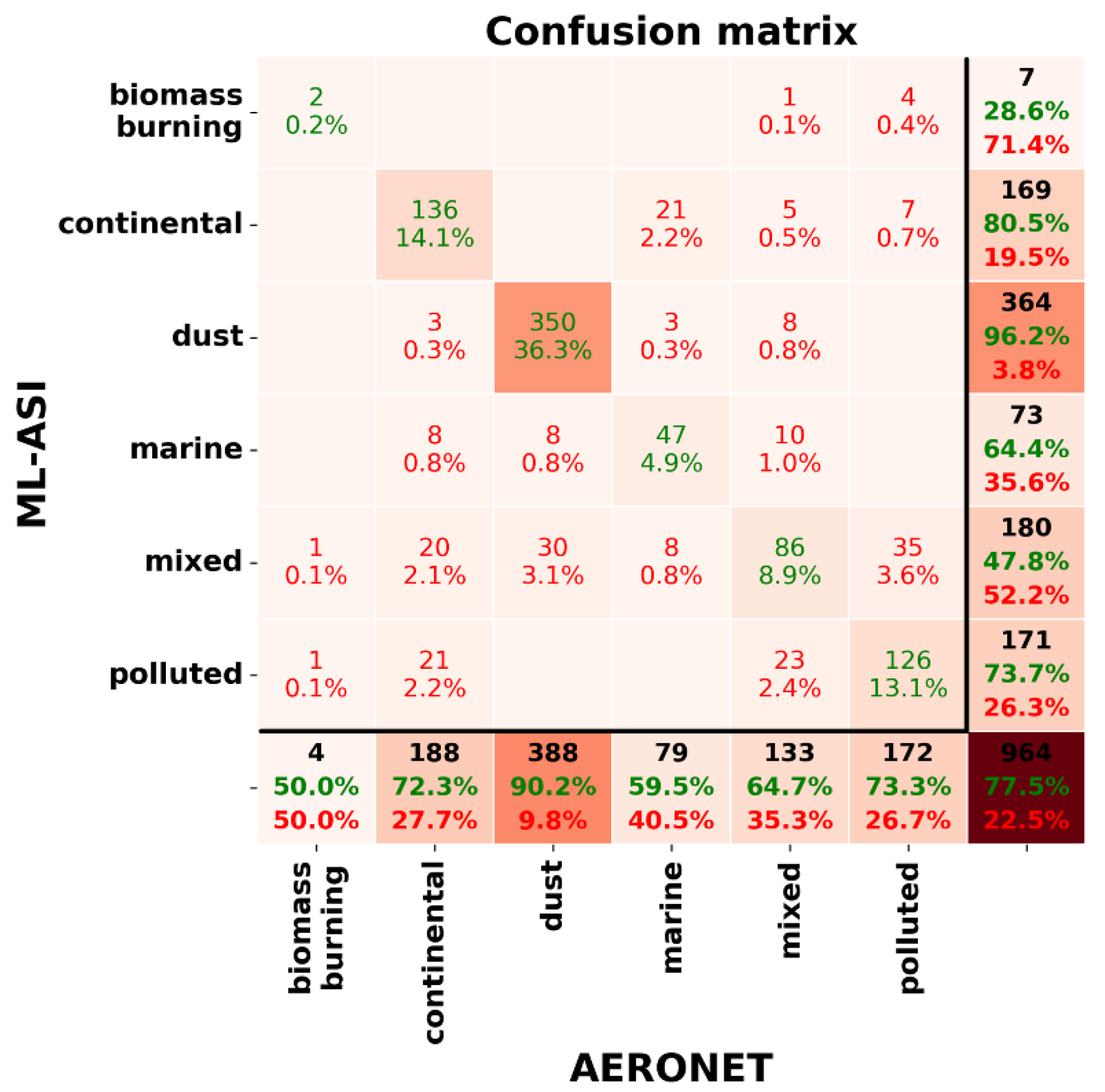
4.2. Aerosol Type Classification
5. Conclusions
Supplementary Materials
Author Contributions
Funding
Informed Consent Statement
Data Availability Statement
Acknowledgments
Conflicts of Interest
Abbreviations
| AOD | Aerosol optical depth |
| AE | Ångström exponent |
| AERONET | AERosol RObotic NETwork |
| ANN | Artificial neural network |
| ASI | All-sky imager |
| DNI | Direct normal irradiance |
| FMF | Fine mode fraction |
| GBM | Gradient boosting machine |
| GHI | Global horizontal irradiance |
| KNN | K-Nearest neighbors |
| LGBM | Light gradient boosting machine |
| MARS | Multivariate adaptive regression splines |
| MBE | Mean bias error |
| ML | Machine learning |
| ML-ASI | ML-ASI retrievals |
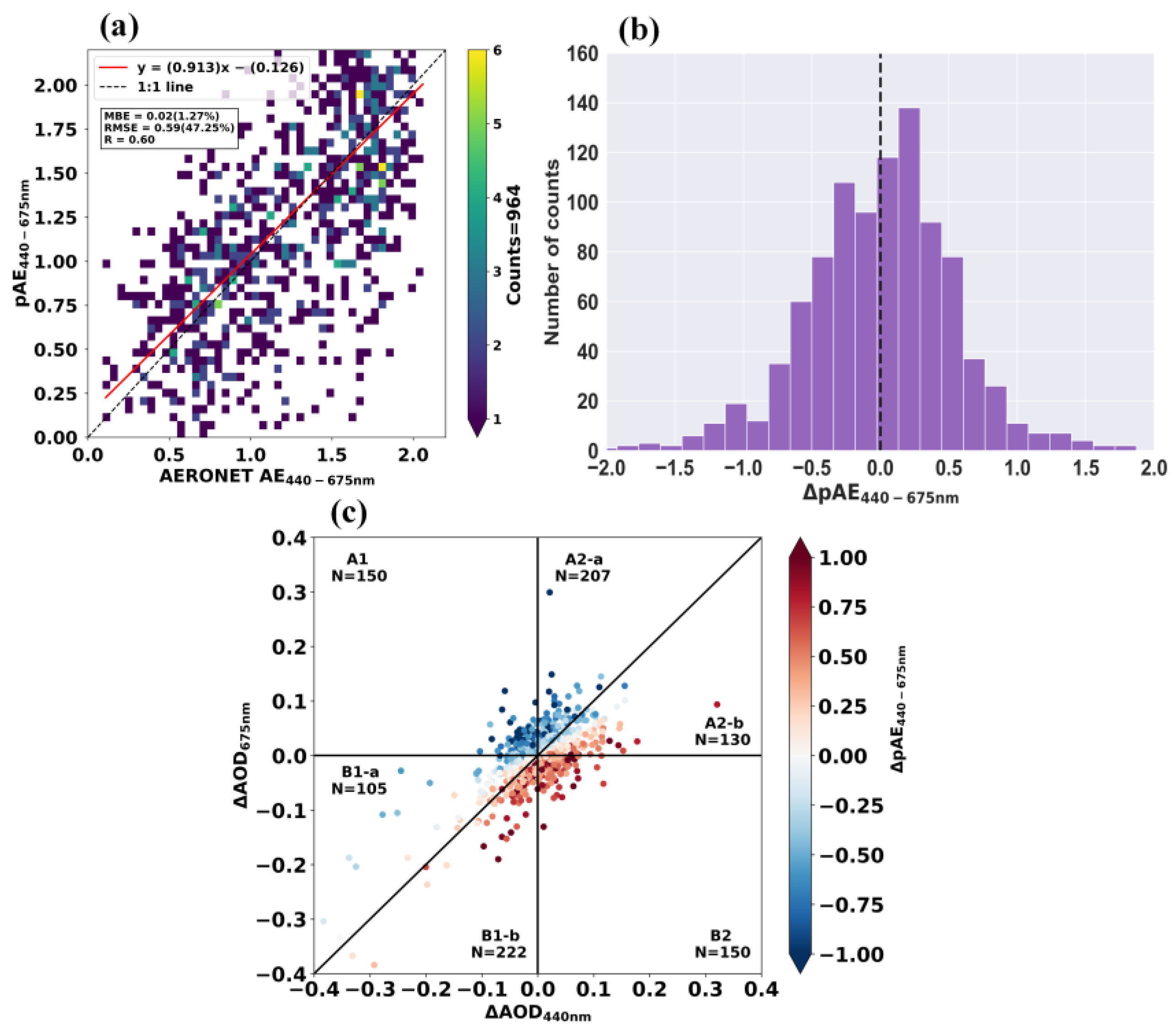
| pAE | AE calculated using Ångström power formula based on ML-ASI AODs |
| rMBE | Relative mean bias error |
| rRMSE | Relative root mean square error |
| RF | Random forest |
| RGB | Red-green-blue |
| RMSE | Root mean square error |
| RTM | Radiative transfer model |
| R | Pearson’s correlation coefficient |
| R2 | Coefficient of determination |
| SAT | Sun-saturated area |
| SVM | Support vector machines |
| SZA | Solar zenith angle |
| TCWV | Total column water vapor |
| XGBoost | Extreme gradient boosting machine |
| Δ | Difference between ML-ASI and AERONET |
References
- Masson-Delmotte, V.; Zhai, P.; Pirani, A.; Connors, S.L.; Péan, C.; Berger, S.; Caud, N.; Chen, Y.; Goldfarb, L.; Gomis, M.I.; et al. Climate Change 2021: The Physical Science Basis. Contribution of Working Group I to the Sixth Assessment Report of the Intergovernmental Panel on Climate Change; Cambridge University Press: Cambridge, UK; New York, NY, USA, 2021. [Google Scholar] [CrossRef]
- Mishchenko, M.; Cairns, B.; Kopp, G.; Schueler, C.F.; Fafaul, B.; Hansen, J.; Hooker, J.; Itchkawich, T.; Maring, H.; Travis, L.D. Accurate monitoring of terrestrial aerosols and total solar irradiance: Introducing the Glory Mission. Bull. Am. Meteorol. Soc. 2007, 88, 677–691. [Google Scholar] [CrossRef] [Green Version]
- Cuneo, L.; Ulke, A.G.; Cerne, B. Advances in the characterization of aerosol optical properties using long-term data from AERONET in Buenos Aires. Atmos. Pollut. Res. 2002, 13, 101360. [Google Scholar] [CrossRef]
- Kaufman, Y.; Tanré, D.; Boucher, O. A satellite view of aerosols in the climate system. Nature 2002, 419, 215–223. [Google Scholar] [CrossRef] [PubMed]
- Eck, T.F.; Holben, B.N.; Sinyuk, A.; Pinker, R.T.; Goloub, P.; Chen, H.; Chatenet, B.; Li, Z.; Singh, R.P.; Tripathi, S.N.; et al. Climatological aspects of the optical properties of fine/coarse mode aerosol mixtures. J. Geophys. Res. Atmos. 2010, 115. [Google Scholar] [CrossRef] [Green Version]
- Liu, Y.; Yi, B. Aerosols over East and South Asia: Type Identification, Optical Properties, and Implications for Radiative Forcing. Remote Sens. 2022, 14, 2058. [Google Scholar] [CrossRef]
- Holben, B.N.; Eck, T.F.; Slutsker, I.; Tanré, D.; Buis, J.P.; Setzer, A.; Vermote, E.; Reagan, J.A.; Kaufman, Y.J.; Nakajima, T.; et al. AERONET—A Federated Instrument Network and Data Archive for Aerosol Characterization. Remote Sens. Environ. 1998, 66, 1–16. [Google Scholar] [CrossRef]
- Remer, L.A.; Kleidman, R.G.; Levy, R.C.; Kaufman, Y.J.; Tanré, D.; Mattoo, S.; Vanderlei, M.; Ichoku, C.; Koren, I.; Yu, H.; et al. Global aerosol climatology from the MODIS satellite sensors. J. Geophys. Res. 2008, 113, D14. [Google Scholar] [CrossRef] [Green Version]
- Levy, R.C.; Mattoo, S.; Munchak, L.A.; Remer, L.A.; Sayer, A.M.; Patadia, F.; Hsu, N.C. The Collection 6 MODIS aerosol products over land and ocean. Atmos. Meas. Tech. 2013, 6, 2989–3034. [Google Scholar] [CrossRef] [Green Version]
- Sayer, A.M.; Hsu, N.C.; Bettenhausen, C.; Jeong, M.J. Validation and uncertainty estimates for MODIS Collection 6 "deep Blue" aerosol data. J. Geophys. Res. Atmos. 2013, 118, 7864–7872. [Google Scholar] [CrossRef] [Green Version]
- Kahn, R.A.; Gaitley, B.J.; Garay, M.J.; Diner, D.J.; Eck, T.F.; Smirnov, A.; Holben, B.N. Multiangle Imaging SpectroRadiometer global aerosol product assessment by comparison with the Aerosol Robotic Network. J. Geophys. Res. Atmos. 2010, 115, D23. [Google Scholar] [CrossRef]
- Mei, L.; Rozanov, V.; Vountas, M.; Burrows, J.P.; Levy, R.C.; Lotz, W. Retrieval of aerosol optical properties using MERIS observations: Algorithm and some first results. Remote Sens. Environ. 2017, 197, 125–140. [Google Scholar] [CrossRef] [PubMed]
- Riffler, M.; Popp, C.; Hauser, A.; Fontana, F.; Wunderle, S. Validation of a modified AVHRR aerosol optical depth retrieval algorithm over Central Europe. Atmos. Meas. Tech. 2010, 3, 1255–1270. [Google Scholar] [CrossRef] [Green Version]
- Prados, A.I.; Kondragunta, S.; Ciren, P.; Knapp, K.R. GOES Aerosol/Smoke Product (GASP) over North America: Comparisons to AERONET and MODIS observations. J. Geophys. Res. 2007, 112, D15201. [Google Scholar] [CrossRef]
- Dubovik, O.; Herman, M.; Holdak, A.; Lapyonok, T.; Tanré, D.; Deuzé, J.L.; Ducos, F.; Sinyuk, A.; Lopatin, A. Statistically optimized inversion algorithm for enhanced retrieval of aerosol properties from spectral multi-angle polarimetric satellite observations. Atmos. Meas. Tech. 2011, 4, 975–1018. [Google Scholar] [CrossRef] [Green Version]
- Sawyer, V.; Levy, R.C.; Mattoo, S.; Cureton, G.; Shi, Y.; Remer, L.A. Continuing the MODIS Dark Target Aerosol Time Series with VIIRS. Remote Sens. 2020, 12, 308. [Google Scholar] [CrossRef] [Green Version]
- King, M.D.; Kaufman, Y.J.; Tanré, D.; Nakajima, T. Remote sensing of tropospheric aerosols from space: Past, present, and future. Bull. Am. Meteorol. Soc. 1999, 80, 2229–2259. [Google Scholar] [CrossRef]
- Li, Z.; Zhao, X.; Kahn, R.; Mishchenko, M.; Remer, L.; Lee, K.H.; Wang, M.; Laszlo, I.; Nakajima, T.; Maring, H. Uncertainties in satellite remote sensing of aerosols and impact on monitoring its long-term trend: A review and perspective. Ann. Geophys. 2009, 27, 2755–2770. [Google Scholar] [CrossRef]
- Bilal, M.; Nichol, J.E.; Chan, P.W. Validation and accuracy assessment of a Simplified Aerosol Retrieval Algorithm (SARA) over Beijing under low and high aerosol loadings and dust storms. Remote Sens. Environ 2014, 153, 50–60. [Google Scholar] [CrossRef]
- Ghonima, M.S.; Urquhart, B.; Chow, C.W.; Shields, J.E.; Cazorla, A.; Kleissl, J. A method for cloud detection and opacity classification based on ground based sky imagery. Atmos. Meas. Tech. 2012, 5, 2881–2892. [Google Scholar] [CrossRef] [Green Version]
- Kazantzidis, A.; Tzoumanikas, P.; Bais, A.F.; Fotopoulos, S.; Economou, G. Cloud detection and classification with the use of whole-sky ground-based images. Atmos. Res. 2012, 113, 80–88. [Google Scholar] [CrossRef]
- Hasenbalg, M.; Kuhn, P.; Wilbert, S.; Nouri, B.; Kazantzidis, A. Benchmarking of six cloud segmentation algorithms for ground-based all-sky imagers. Sol. Energy 2020, 201, 596–614. [Google Scholar] [CrossRef]
- Fabel, Y.; Nouri, B.; Wilbert, S.; Blum, N.; Triebel, R.; Hasenbalg, M.; Kuhn, P.; Zarzalejo, L.F.; Pitz-Paal, R. Applying self-supervised learning for semantic cloud segmentation of all-sky images. Atmos. Meas. Tech. 2022, 15, 797–809. [Google Scholar] [CrossRef]
- Cheng, H.Y.; Yu, C.C. Block-based cloud classification with statistical features and distribution of local texture features. Atmos. Meas. Tech. 2015, 8, 1173–1182. [Google Scholar] [CrossRef] [Green Version]
- Taravat, A.; Del Frate, F.; Cornaro, C.; Vergari, S. Neural networks and support vector machine algorithms for automatic cloud classification of whole-sky ground-based images. IEEE Geosci. Remote Sens. Lett. 2015, 12, 666–670. [Google Scholar] [CrossRef]
- Zhang, J.; Liu, P.; Zhang, F.; Song, Q. CloudNet: Ground-Based Cloud Classification with Deep Convolutional Neural Network. Geophys. Res. Lett. 2018, 45, 8665–8672. [Google Scholar] [CrossRef]
- Ye, L.; Cao, Z.; Xiao, Y.; Yang, Z. Supervised Fine-Grained Cloud Detection and Recognition in Whole-Sky Images. IEEE Trans. Geosci. Remote Sens. 2019, 57, 7972–7985. [Google Scholar] [CrossRef]
- Blanc, P.; Massip, P.; Kazantzidis, A.; Tzoumanikas, P.; Kuhn, P.; Wilbert, S.; Schüler, D.; Prahl, C. Short-term forecasting of high resolution local DNI maps with multiple fisheye cameras in stereoscopic mode. AIP Conf. Proc. 2017, 1850, 140004. [Google Scholar] [CrossRef] [Green Version]
- Kuhn, P.; Nouri, B.; Wilbert, S.; Prahl, C.; Kozonek, N.; Schmidt, T.; Yasser, Z.; Ramirez, L.; Zarzalejo, L.; Meyer, A.; et al. Validation of an all-sky imager–based nowcasting system for industrial PV plants. Prog. Photovoltaics Res. Appl. 2018, 26, 608–621. [Google Scholar] [CrossRef]
- Nouri, B.; Kuhn, P.; Wilbert, S.; Hanrieder, N.; Prahl, C.; Zarzalejo, L.; Kazantzidis, A.; Blanc, P.; Pitz-Paal, R. Cloud height and tracking accuracy of three all sky imager systems for individual clouds. Sol. Energy 2019, 177, 213–228. [Google Scholar] [CrossRef] [Green Version]
- Crisosto, C.; Hofmann, M.; Mubarak, R.; Seckmeyer, G. One-hour prediction of the global solar irradiance from all-sky images using artificial neural networks. Energies 2018, 11, 2906. [Google Scholar] [CrossRef] [Green Version]
- Kamadinata, J.O.; Ken, T.L.; Suwa, T. Sky image-based solar irradiance prediction methodologies using artificial neural networks. Renew. Energy 2019, 134, 837–845. [Google Scholar] [CrossRef]
- Jiang, J.; Lv, Q.; Gao, X. The ultra-short-term forecasting of global horizonal irradiance based on total sky images. Remote Sens. 2020, 12, 3671. [Google Scholar] [CrossRef]
- Nouri, B.; Blum, N.; Wilbert, S.; Zarzalejo, L.F. A hybrid solar irradiance nowcasting approach: Combining all sky imager systems and persistence irradiance models for increased accuracy. Sol. RRL 2021, 6, 2100442. [Google Scholar] [CrossRef]
- Logothetis, S.A.; Salamalikis, V.; Nouri, B.; Remund, J.; Zarzalejo, L.; Xie, Y.; Wilbert, S.; Ntavelis, E.; Nou, J.; Hendrikx, E.; et al. Benchmarking of solar irradiance nowcast performance derived from all-sky imagers. Renew. Energy 2022, 199, 246–261. [Google Scholar] [CrossRef]
- Chu, Y.; Pedro, H.T.C.; Li, M.; Coimbra, C.F.M. Real-time forecasting of solar irradiance ramps with smart image processing. Sol. Energy 2015, 114, 91–104. [Google Scholar] [CrossRef]
- Caldas, M.; Alonso-Suárez, R. Very short-term solar irradiance forecast using all-sky imaging and real-time irradiance measurements. Renew. Energy 2019, 143, 1643–1658. [Google Scholar] [CrossRef]
- Logothetis, S.A.; Salamalikis, V.; Wilbert, S.; Remund, J.; Zarzalejo, L.; Xie, Y.; Nouri, B.; Ntavelis, E.; Nou, J.; Hendrikx, E.; et al. Solar irradiance ramp forecasting based on all-sky imagers. Energies 2022, 15, 6191. [Google Scholar] [CrossRef]
- Dev, S.; Savoy, F.M.; Lee, Y.H.; Winkler, S. Estimating solar irradiance using sky imagers. Atmos. Meas. Tech. 2019, 12, 5417–5429. [Google Scholar] [CrossRef] [Green Version]
- Chu, Y.; Li, M.; Pedro, H.T.C.; Coimbra, C.F.M. A network of sky imagers for spatial solar irradiance assessment. Renew. Energy 2022, 187, 1009–1019. [Google Scholar] [CrossRef]
- Olmo, F.J.; Cazorla, A.; Alados-Arboledas, L.; López-Álvarez, M.A.; Hernández-Andrés, J.; Romero, J. Retrieval of the optical depth using an all-sky CCD camera. Appl. Opt. 2008, 47, 34. [Google Scholar] [CrossRef]
- Cazorla, A.; Shields, J.E.; Karr, M.E.; Olmo, F.J.; Burden, A.; Alados-Arboledas, L. Technical Note: Determination of aerosol optical properties by a calibrated sky imager. Atmos. Chem. Phys. 2009, 9, 6417–6427. [Google Scholar] [CrossRef] [Green Version]
- Huo, J.; Lu, D.R. Preliminary retrieval of aerosol optical depth from all-sky images. Adv. Atmos. Sci. 2010, 27, 421–426. [Google Scholar] [CrossRef]
- Berk, A.; Anderson, G.; Acharya, P.; Bernstein, L.; Muratov, L.; Lee, J.; Fox, M.; Adler-Golden, S.; Chetwynd, J.; Hoke, M.; et al. MODTRAN5: A reformulated atmospheric band model with auxiliary species and practical multiple scattering options. Proc. SPIE 2005, 5655, 88–95. [Google Scholar] [CrossRef]
- Servera, J.V.; Rivera-Caicedo, J.P.; Verrelst, J.; Muñoz-Marí, J.; Sabater, N.; Berthelot, B.; Camps-Valls, G.; Moreno, J. Systematic Assessment of MODTRAN Emulators for Atmospheric Correction. IEEE Trans. Geosci. Remote Sens. 2021, 60, 4101917. [Google Scholar] [CrossRef]
- Kazantzidis, A.; Tzoumanikas, P.; Nikitidou, E.; Salamalikis, V.; Wilbert, S.; Prahl, C. Application of Simple All-sky Imagers for the Estimation of Aerosol Optical Depth. AIP Conf. Proc. 2017, 1850, 140012. [Google Scholar] [CrossRef] [Green Version]
- Mayer, B.; Kylling, A. Technical note: The libRadtran software package for radiative transfer calculations e description and examples of use. Atmos. Chem. Phys. 2005, 5, 1855–1877. [Google Scholar] [CrossRef] [Green Version]
- Dubovik, O.; Lapyonok, T.; Litvinov, P.; Herman, M.; Fuertes, D.; Ducos, F.; Lopatin, A.; Chaikovsky, A.; Torres, B.; Derimian, Y.; et al. GRASP: A versatile algorithm for characterizing the atmosphere. SPIE Newsroom 2014, 25, 2-1201408. [Google Scholar] [CrossRef]
- Román, R.; Antuña-Sánchez, J.C.; Cachorro, V.E.; Toledano, C.; Torres, B.; Mateos, D.; Fuertes, D.; López, C.; González, R.; Lapionok, T.; et al. Retrieval of aerosol properties using relative radiance measurements from an all-sky camera. Atmos. Meas. Tech. 2022, 15, 407–433. [Google Scholar] [CrossRef]
- Antuña-Sánchez, J.C.; Román, R.; Cachorro, V.E.; Toledano, C.; López, C.; González, R.; Mateos, D.; Calle, A.; de Frutos, Á.M. Relative sky radiance from multi-exposure all-sky camera images. Atmos. Meas. Tech. 2021, 14, 2201–2217. [Google Scholar] [CrossRef]
- Scarlatti, F.; Gómez-Amo, J.L.; Valdelomar, P.C.; Estellés, V.; Utrillas, M.P. A Machine Learning Approach to Derive Aerosol Properties from All-Sky Camera Imagery. Remote Sens. 2023, 15, 1676. [Google Scholar] [CrossRef]
- Gueymard, C.A. Temporal variability in direct and global irradiance at various time scales as affected by aerosols. Sol. Energy 2012, 86, 3544–3553. [Google Scholar] [CrossRef]
- Vamvakas, I.; Salamalikis, V.; Benitez, D.; Al-Salaymeh, A.; Bouaichaoui, S.; Yassaa, N.; Guizani, A.; Kazantzidis, A. Estimation of global horizontal irradiance using satellite-derived data across Middle East-North Africa: The role of aerosol optical properties and site-adaptation methodologies. Renew. Energy 2020, 157, 312–331. [Google Scholar] [CrossRef]
- Ruiz-Arias, J.A.; Gueymard, C.A. Worldwide inter-comparison of clear-sky solar radiation models: Consensus-based review of direct and global irradiance components simulated at the earth surface. Sol. Energy 2018, 168, 10–29. [Google Scholar] [CrossRef]
- Book, H.; Poikonen, A.; Aarva, A.; Mielonen, T.; Pitkanen, M.R.A.; Lindfors, A.V. Photovoltaic system modeling: A validation study at high latitudes with implementation of a novel DNI quality control method. Sol. Energy 2020, 204, 316–329. [Google Scholar] [CrossRef]
- Abreu, E.F.; Gueymard, C.A.; Canhoto, P.; Costa, M.J. Performance assessment of clear-sky solar irradiance predictions using state-of-the-art radiation models and input atmospheric data from reanalysis or ground measurements. Sol. Energy 2023, 252, 309–321. [Google Scholar] [CrossRef]
- Seinfeld, J.H.; Pandis, S.N. Atmospheric Chemistry and Physics from Air Pollution to Climate Change; John Wiley & Sons, Inc.: Hoboken, NJ, USA, 2006. [Google Scholar] [CrossRef]
- Dubovik, O.; Holben, B.; Eck, T.F.; Smirnov, A.; Kaufman, Y.G.; King, M.D.; Tanre, D.; Slutsker, I. Variability of Absorption and Optical Properties of Key Aerosol Types Observed in Worldwide Locations. J. Atmos. Sci. 2002, 59, 590–608. [Google Scholar] [CrossRef]
- Lee, J.; Kim, J.; Song, C.H.; Kim, S.B.; Chun, Y.; Sohn, B.J.; Holben, B.N. Characteristics of aerosol types from AERONET sunphotometer measurements. Atmos. Environ. 2010, 44, 3110–3117. [Google Scholar] [CrossRef]
- Giles, D.M.; Holben, B.N.; Eck, T.F.; Sinyuk, A.; Smirnov, A.; Slutsker, I.; Dickerson, R.R.; Thompson, A.M.; Schafer, J.S. An analysis of AERONET aerosol absorption properties and classifications representative of aerosol source regions. J. Geophys. Res. Atmos. 2012, 117. [Google Scholar] [CrossRef] [Green Version]
- Che, H.; Qi, B.; Zhao, H.; Xia, X.; Eck, T.F.; Goloub, P.; Dubovik, O.; Estelles, V.; Cuevas-Agulló, E.; Blarel, L.; et al. Aerosol optical properties and direct radiative forcing based on measurements from the China Aerosol Remote Sensing Network (CARSNET) in eastern China. Atmos. Chem. Phys. 2018, 18, 405–425. [Google Scholar] [CrossRef] [Green Version]
- Logothetis, S.-A.; Salamalikis, V.; Kazantzidis, A. Aerosol classification in Europe, Middle East, North Africa and Arabian Peninsula based on AERONET Version 3. Atmos. Res. 2020, 239, 104893. [Google Scholar] [CrossRef]
- Logothetis, S.-A.; Salamalikis, V.; Kazantzidis, A. The impact of different aerosol properties and types on direct aerosol radiative forcing and efficiency using AERONET Version 3. Atmos. Res. 2021, 250, 105343. [Google Scholar] [CrossRef]
- Lin, J.; Zheng, Y.L.; Shen, X.; Xing, L.; Che, H. Global Aerosol Classification Based on Aerosol Robotic Network (AERONET) and Satellite Observation. Remote Sens. 2021, 13, 1114. [Google Scholar] [CrossRef]
- Gerasopoulos, E.; Amiridis, V.; Kazadzis, S.; Kokkalis, P.; Eleftheratos, K.; Andreae, M.O.; Andreae, T.W. Three-year ground-based measurements of aerosol optical depth over the Eastern Mediterranean: The urban environment of Athens. Atmos. Chem. Phys. 2011, 11, 2145–2159. [Google Scholar] [CrossRef] [Green Version]
- Eleftheriadis, K.; Colbeck, I.; Housiadas, C.; Lazaridis, M.; Mihalopoulos, N.; Mitsakou, C.; Smolik, J.; Ždímal, V. Size distribution, composition and origin of the submicron aerosol in the marine boundary layer during the eastern Mediterranean “SUB-AERO” experiment. Atmos. Environ. 2006, 40, 6245–6260. [Google Scholar] [CrossRef]
- Athanasopoulou, E.; Speyer, O.; Brunner, D.; Vogel, H.; Vogel, B.; Mihalopoulos, N.; Gerasopoulos, E. Changes in domestic heating fuel use in Greece: Effects on atmospheric chemistry and radiation. Atmos. Chem. Phys. 2017, 17, 10597–10618. [Google Scholar] [CrossRef] [Green Version]
- Amiridis, V.; Zerefos, C.; Kazadzis, S.; Gerasopoulos, E.; Eleftheratos, K.; Vrekoussis, M.; Stohl, A.; Mamouri, R.E.; Kokkalis, P.; Papayannis, A.; et al. Impact of the 2009 Attica wild fires on the air quality in urban Athens. Atmos. Environ. 2012, 46, 536–544. [Google Scholar] [CrossRef]
- Masoom, A.; Fountoulakis, I.; Kazadzis, S.; Raptis, I.-P.; Kampouri, A.; Psiloglou, B.; Kouklaki, D.; Papachristopoulou, K.; Marinou, E.; Solomos, S.; et al. Investigation of the effects of the Greek extreme wildfires of August 2021 on air quality and spectral solar irradiance. EGUsphere 2023. [CrossRef]
- Eleftheriadis, K. Long term variability of the air pollution sources reflected on the state of mixing of the urban aerosol. Environ. Sci. Health 2019, 8, 36–39. [Google Scholar] [CrossRef]
- Tsiflikiotou, M.A.; Kostenidou, E.; Papanastasiou, D.K.; Patoulias, D.; Zarmpas, P.; Paraskevopoulou, D.; Diapouli, E.; Kalt-sonoudis, C.; Florou, K.; Bougiatioti, A.; et al. Summertime particulate matter and its composition in Greece. Atmos. Environ. 2019, 213, 597–607. [Google Scholar] [CrossRef]
- Raptis, I.-P.; Kazadzis, S.; Amiridis, V.; Gkikas, A.; Gerasopoulos, E.; Mihalopoulos, N. A Decade of Aerosol Optical Properties Measurements over Athens, Greece. Atmosphere 2020, 11, 154. [Google Scholar] [CrossRef] [Green Version]
- Barreto, A.; Cuevas, E.; Granados-Munoz, M.-J.; Alados-Arboledas, L.; Romero, P.M.; Grobner, J.; Kouremeti, N.; Almansa, A.F.; Stone, T.; Toledano, C.; et al. The new sun-sky-lunar Cimel CE318-T multiband photometer—A comprehensive performance evaluation. Atmos. Meas. Tech. 2016, 9, 631–654. [Google Scholar] [CrossRef] [Green Version]
- Giles, D.M.; Sinyuk, A.; Sorokin, M.G.; Schafer, J.S.; Smirnov, A.; Slutsker, I.; Eck, T.F.; Holben, B.N.; Lewis, J.R.; Campbell, J.R.; et al. Advancements in the Aerosol Robotic Network (AERONET) Version 3 database—Automated near-real-time quality control algorithm with improved cloud screening for Sun photometer aerosol optical depth (AOD) measurements. Atmos. Meas. Tech. 2019, 12, 169–209. [Google Scholar] [CrossRef] [Green Version]
- Smirnov, A.; Holben, B.N.; Lyapustin, A.; Slutsker, I.; Eck, T.F. AERONET processing algorithms refinement. In Proceedings of the AERONET2004 Workshop, El Arenosillo, Spain, 10–14 May 2004; pp. 10–14. [Google Scholar]
- Dubovik, O.; King, M.D. A flexible inversion algorithm for retrieval of aerosol optical properties from sun and sky radiance measurements. J. Geophys. Res. 2000, 105, 20673–20696. [Google Scholar] [CrossRef] [Green Version]
- Friedman, J.H. Greedy Function Approximation: A Gradient Boosting Machine. Ann. Stat. 2001, 29, 1189–1232. [Google Scholar] [CrossRef]
- Ke, G.; Meng, Q.; Finley, T.; Wang, T.; Chen, W.; Ma, W.; Ye, Q.; Liu, T.Y. LightGBM: A Highly Efficient Gradient Boosting Decision Tree. Adv. Neural Inf. Process. Syst. 2017, 9, 3147–3155. Available online: https://dl.acm.org/doi/10.5555/3294996.3295074 (accessed on 28 June 2023).
- Torres, B.; Dubovik, O.; Toledano, C.; Berjon, A.; Cachorro, V.E.; Lapyonok, T.; Litvinov, P.; Goloub, P. Sensitivity of aerosol retrieval to geometrical configuration of ground-based sun/sky radiometer observations. Atmos. Chem. Phys. 2014, 14, 847–875. [Google Scholar] [CrossRef]
- Wriedt, T. Mie Theory: A Review. In The Mie Theory: Basics and Applications; Springer Series in Optical Sciences; Springer: Berlin/Heidelberg, Germany, 2012; p. 169. [Google Scholar] [CrossRef]
- Rubin, J.I.; Reid, J.S.; Xian, P.; Selman, C.M.; Eck, T.F. A global evaluation of daily to seasonal aerosol and water vapor relationships using a combination of AERONET and NAAPS reanalysis data. Atmos. Chem. Phys. 2023, 23, 4059–4090. [Google Scholar] [CrossRef]
- Inness, A.; Ades, M.; Agustí-Panareda, A.; Barré, J.; Benedictow, A.; Blechschmidt, A.M.; Dominguez, J.J.; Engelen, R.; Eskes, H.; Flemming, J.; et al. The CAMS reanalysis of atmospheric composition. Atmos. Chem. Phys. 2019, 19, 3515–3556. [Google Scholar] [CrossRef] [Green Version]
- O’Neill, N.T.; Dubovik, O.; Eck, T.F. Modified Ångström Exponent for the Characterization of Submicrometer Aerosols. Appl. Opt. 2001, 40, 2368–2375. [Google Scholar] [CrossRef]
- Gkikas, A.; Basart, S.; Hatzianastassiou, N.; Marinou, E.; Amiridis, V.; Kazadzis, S.; Pey, J.; Querol, X.; Jorba, O.; Gassó, S.; et al. Mediterranean intense desert dust outbreaks and their vertical structure based on remote sensing data. Atmos. Chem. Phys. 2016, 16, 8609–8642. [Google Scholar] [CrossRef] [Green Version]


| Variable | MBE (rMBE) | RMSE (rRMSE) | R |
|---|---|---|---|
| AOD440 nm | −0.0012 (−0.51%) | 0.056 (23.1%) | 0.93 |
| AOD500 nm | 0.000069 (0.033%) | 0.066 (32.4%) | 0.89 |
| AOD675 nm | −0.0011 (−0.71%) | 0.053 (33.9%) | 0.92 |
| Variable | MBE (rMBE) | RMSE (rRMSE) | R |
|---|---|---|---|
| AE440–675 nm | 0.017 (1.4%) | 0.15 (12.0%) | 0.92 |
| FMF500 nm | 0.007 (1.2%) | 0.057 (9.67%) | 0.95 |
Disclaimer/Publisher’s Note: The statements, opinions and data contained in all publications are solely those of the individual author(s) and contributor(s) and not of MDPI and/or the editor(s). MDPI and/or the editor(s) disclaim responsibility for any injury to people or property resulting from any ideas, methods, instructions or products referred to in the content. |
© 2023 by the authors. Licensee MDPI, Basel, Switzerland. This article is an open access article distributed under the terms and conditions of the Creative Commons Attribution (CC BY) license (https://creativecommons.org/licenses/by/4.0/).
Share and Cite
Logothetis, S.-A.; Giannaklis, C.-P.; Salamalikis, V.; Tzoumanikas, P.; Raptis, P.-I.; Amiridis, V.; Eleftheratos, K.; Kazantzidis, A. Aerosol Optical Properties and Type Retrieval via Machine Learning and an All-Sky Imager. Atmosphere 2023, 14, 1266. https://doi.org/10.3390/atmos14081266
Logothetis S-A, Giannaklis C-P, Salamalikis V, Tzoumanikas P, Raptis P-I, Amiridis V, Eleftheratos K, Kazantzidis A. Aerosol Optical Properties and Type Retrieval via Machine Learning and an All-Sky Imager. Atmosphere. 2023; 14(8):1266. https://doi.org/10.3390/atmos14081266
Chicago/Turabian StyleLogothetis, Stavros-Andreas, Christos-Panagiotis Giannaklis, Vasileios Salamalikis, Panagiotis Tzoumanikas, Panagiotis-Ioannis Raptis, Vassilis Amiridis, Kostas Eleftheratos, and Andreas Kazantzidis. 2023. "Aerosol Optical Properties and Type Retrieval via Machine Learning and an All-Sky Imager" Atmosphere 14, no. 8: 1266. https://doi.org/10.3390/atmos14081266