5.1. SBL Low-Order Moments
The advent of high-performance computing allows mesh convergence to be studied using 3D simulations. Solution convergence in LES is complicated by the mesh dependence in the SFS model, e.g., holding the domain size fixed, the resolved flux in a
simulation is of course different than the resolved flux in a
simulation. Judging convergence in LES is also challenging as the subgrid-scale model and numerical discretization errors are intertwined since both depend explicitly on the mesh spacing [
51]. Here we use physically based metrics based on the vertical profiles of low-order statistical moments to judge convergence, as discussed in Sullivan and Patton [
52] for convectively driven boundary layers; also see Geurts and Fröhlich [
53].
Table 1 provides a summary of the bulk parameters for SBL simulations with
K h
, grid meshes
,
K h
,
. The variables in
Table 1 are the LES case, grid mesh points
N, mesh spacing ▵, cooling rate
, friction velocity
, surface temperature flux
, boundary-layer depth
h, Monin–Obukhov stability length
with von Kármán constant
, and boundary-layer stability
. The SBL depth
h is defined as the vertical location where the vertical gradient of temperature
reaches a maximum (see [
20,
54]). There is variation in
with the grid resolution because of variability in the SBL depth
h. Dai et al. [
55] speculates that this is a consequence of the stability length-scale correction used in the LES. Statistics, denoted by angle brackets
, are formed by averaging in the
planes and over the time period
h, except for simulation C2, which used a shorter 30 min time average. A turbulent fluctuation from a horizontal mean is denoted by a superscript prime
.
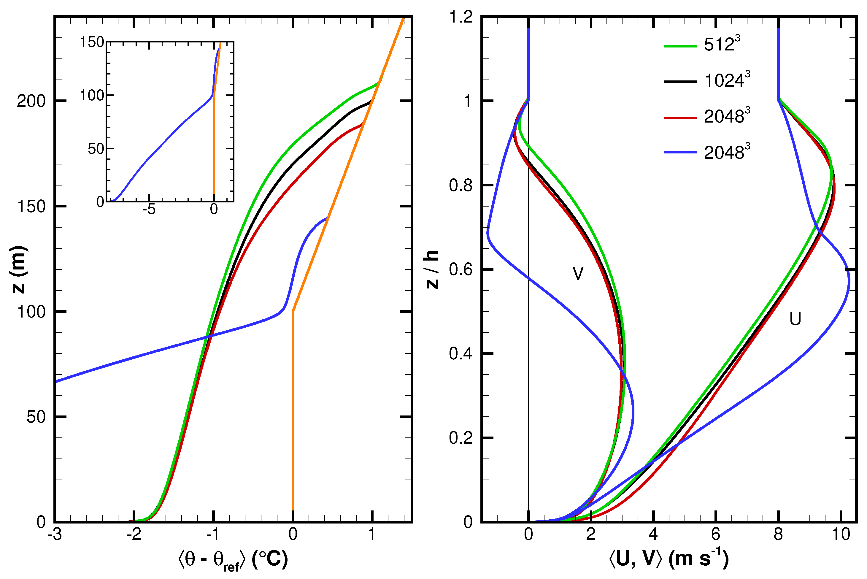
Figure 2 compares the profiles of winds and temperature for three different resolutions
with fixed surface cooling
K h
. To eliminate the slight variability with the boundary-layer depth we introduce the dimensionless vertical coordinate
, as shown in the right panel of
Figure 2. The flux and variance profiles are normalized by the surface values
as appropriate. Under this normalization the wind profiles collapse well (the right panel of
Figure 2). The low-level jet is positioned at
and its magnitude is 1.2
.
Figure 2.
Vertical profiles of average temperature (left panel). Simulations (B, C, C2) with cooling rate K h and are represented by line colors (green, black, red), respectively. Simulation F2 with K h and is presented in blue. The inset figure shows the variation of temperature in F2 in the lower SBL. The initial temperature field at is shown as the orange line and K. Vertical profiles of average winds are shown in the right panel. Note that the vertical coordinate for the wind profiles is normalized by the SBL height h from each simulation.
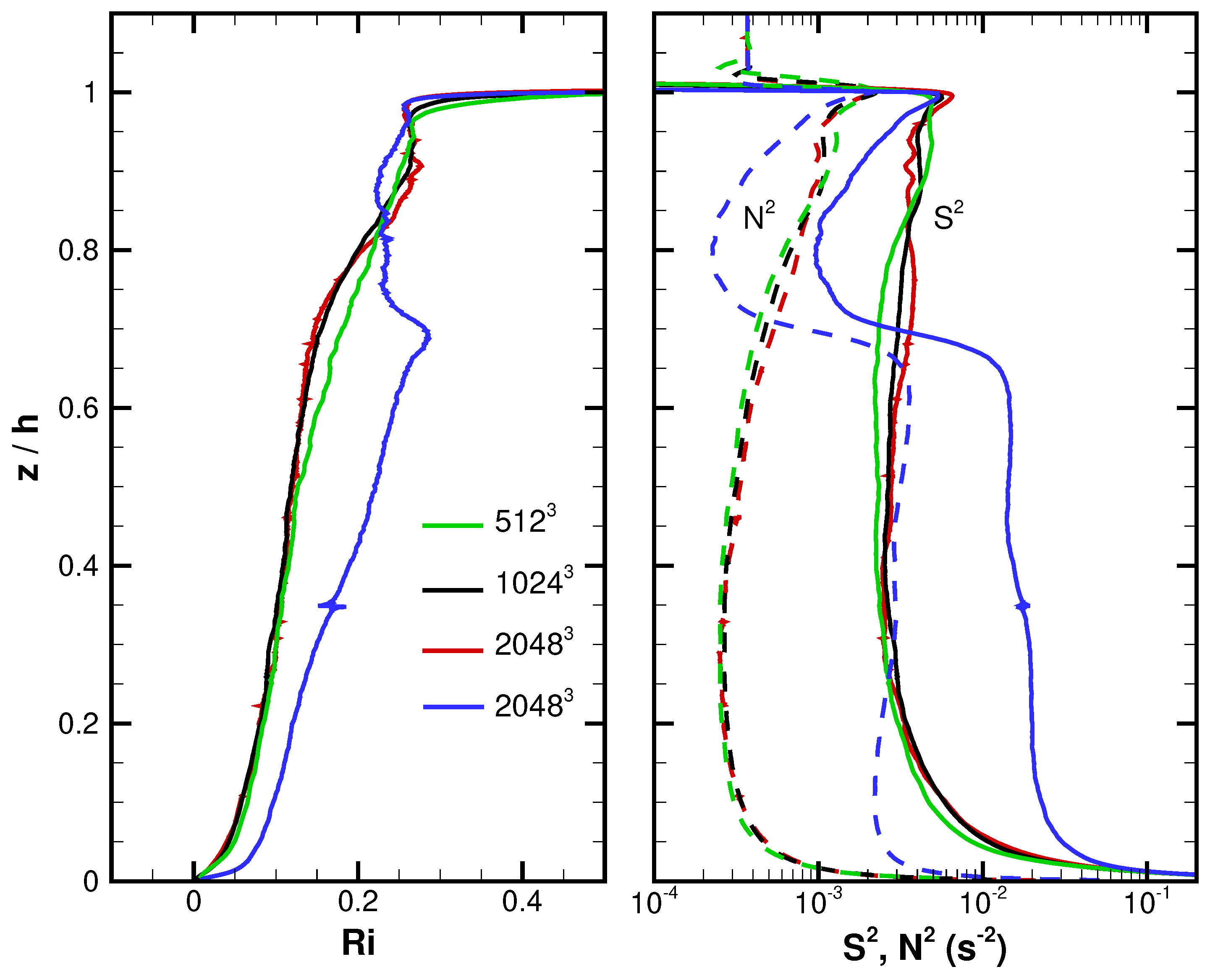
The vertical profiles of the Richardson number
and the squared shear and buoyancy frequency
are displayed in
Figure 3 for the three resolutions considered. Here
where the horizontal wind aligned with the mean wind direction is given by
. The profiles of
are very well converged for the three different mesh resolutions below
. In the upper SBL, above the low-level jet the profiles for simulations C2 and C are converged. These profiles show that the simulation is in the weakly stable regime as in Sullivan et al. [
20]. In particular, the profile
shows the approximate validity of the very simple RANS parameterization of a constant Richardson number above the Monin–Obukhov surface layer.
Figure 3.
Vertical profiles of average Richardson number (left panel). Simulations with cooling rate K h (B, C, C2) with are denoted by line colors (green, black, red), respectively. Simulation F2 with K h and is presented in blue. Vertical profiles of average shear and buoyancy frequency squared , indicated by (solid, dashed) lines, respectively, are shown in the right panel.
Figure 2 and
Figure 3 also illustrate a strong dependence on bulk stratification in the SBL. The bulk stability measure
increases from 1.56 to 5.77 as the cooling rate varies from
to 1 K h
. Increasing stratification leads to a decrease in the SBL turbulence level and as a result the height of the low-level jet (LLJ) descends from
to 0.58, i.e., from 105 m to 83 m. Then the wind veering in F2 is sharper and compressed in the lower SBL compared to C2. In F2, notice that the SBL is nearly equally split between the vertical layers below and above the LLJ. The mean wind, temperature, shear, and buoyancy profiles all change markedly above the LLJ compared to their counterparts in the lower SBL. Compensating for changes in the shear and buoyancy profiles leads to a relatively uniform
profile above the LLJ, which supports weak stratified turbulence. A further discussion of the impacts of increasing stratification on SBL statistics is given in [
20].
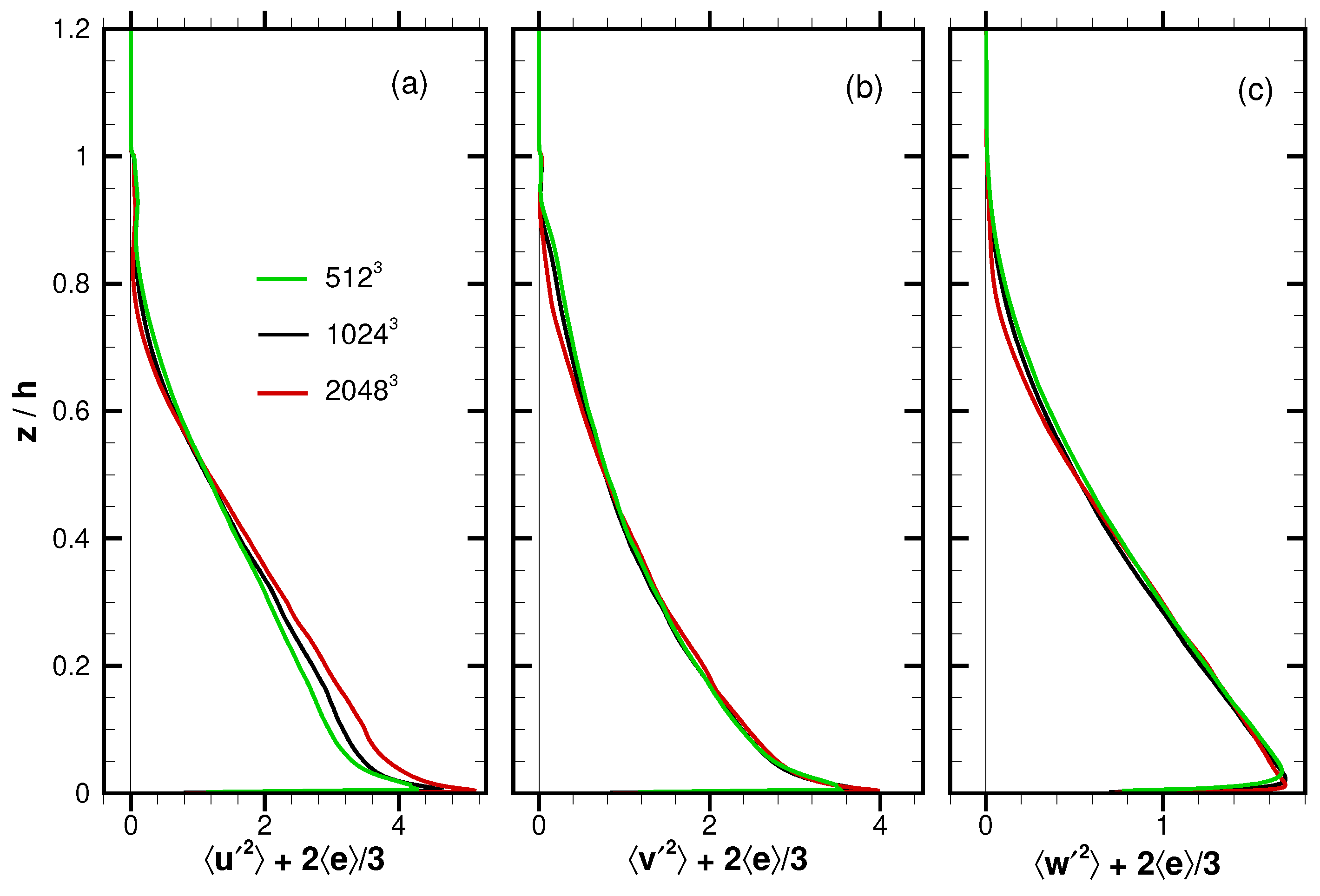
The velocity variances from simulations (B, C, C2), which include the SFS contribution
, collapse reasonably well for the three mesh resolutions considered, as shown in
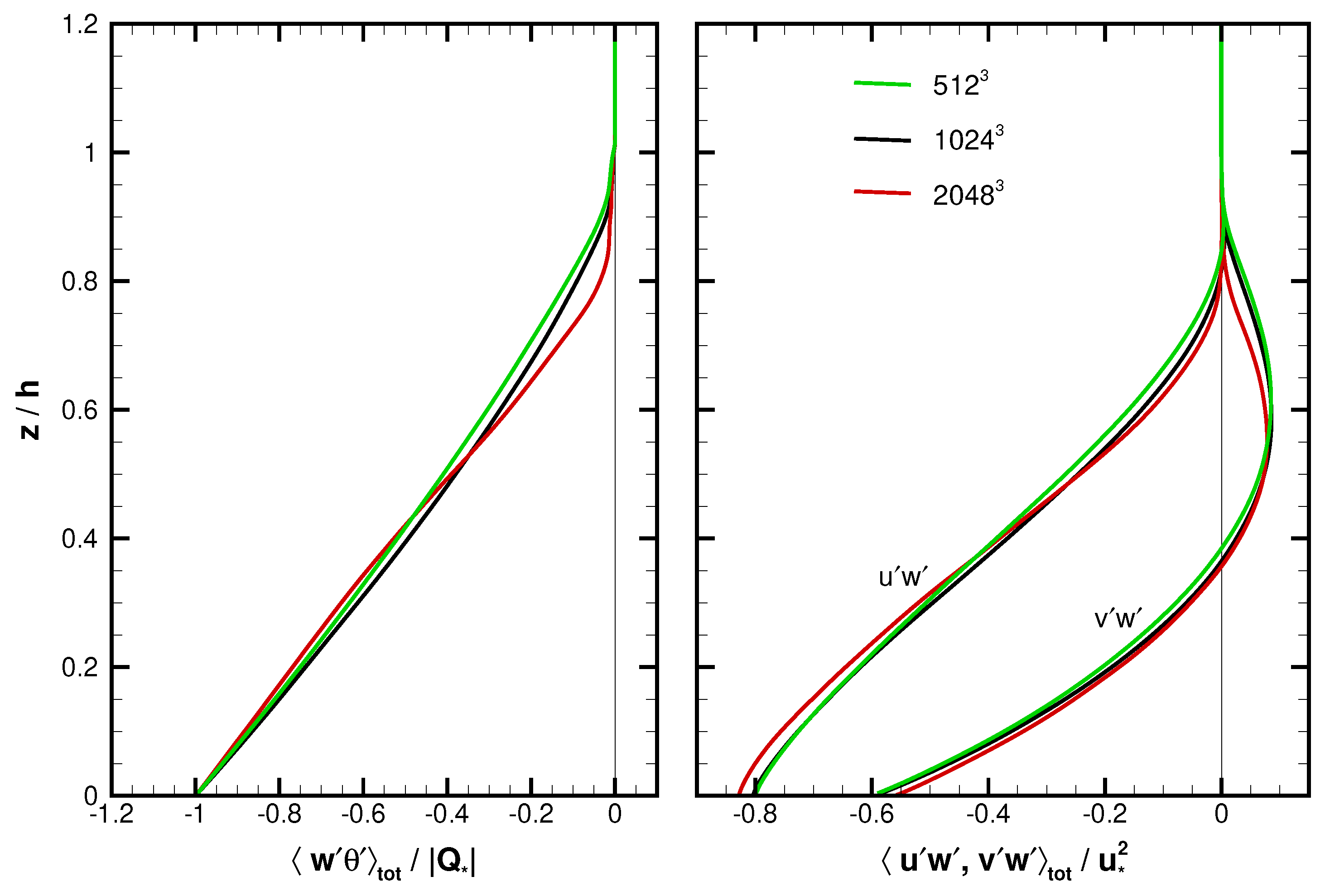
Figure 4. The momentum and temperature fluxes
that include both the resolved and SFS contributions are in close agreement as the mesh spacing varies from
; see
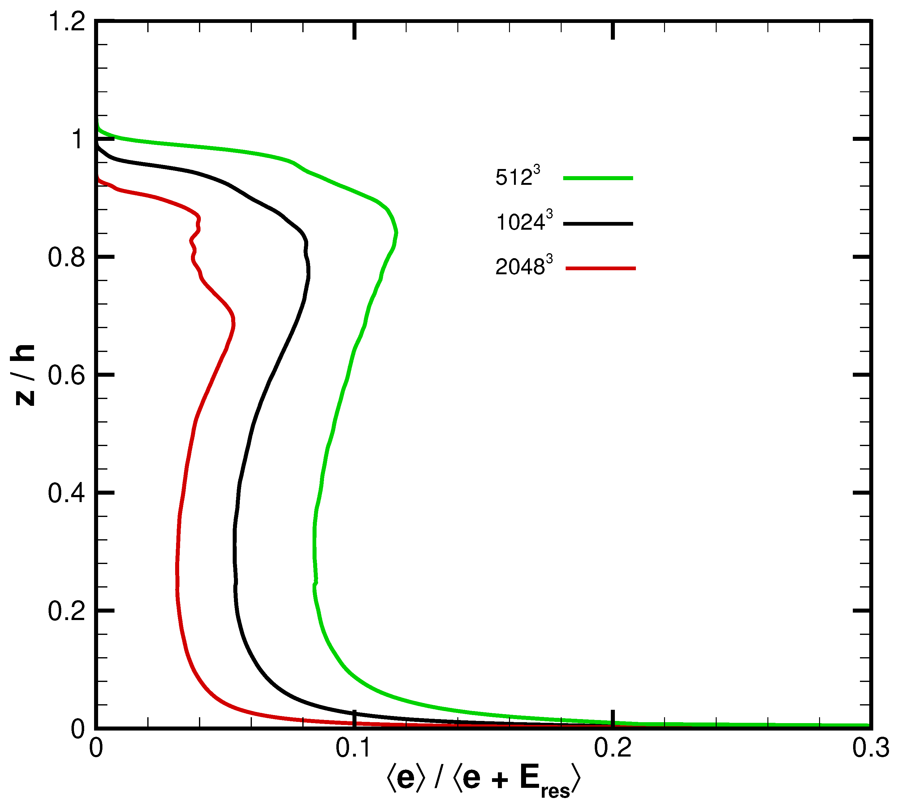
Figure 5. The profile of SFS energy
, shown in
Figure 6, shows a systematic decrease with resolution over the bulk of the SBL. For example, at
the scaling relationship
holds [
36] (p. 589). The results in
Figure 6 find a 40% decrease in
e for a mesh-size reduction from 0.78 m to 0.2 m. Based on these results, we judge the LES results to be well converged.
Figure 4.
Vertical profiles of velocity variances (panels (a)–(c), respectively). The variances include an estimate of the SFS contribution . Results are from simulations (B, C, C2) with denoted by line colors (green, black, red), respectively. The vertical coordinate is normalized by the SBL height h from each simulation.
Figure 5.
Vertical profiles of average temperature flux (left panel) and momentum fluxes (right panel). The fluxes are normalized by and as appropriate. The fluxes include the SFS contributions. Results are from simulations (B, C, C2) with , denoted by line colors (green, black, red), respectively. The vertical coordinate is normalized by the SBL height h from each simulation.
Figure 6.
Vertical profile of SFS energy in the LES as a fraction of the total energy for different meshes denoted by (green, black, red) lines, respectively. The resolved kinetic energy .
Figure 6.
Vertical profile of SFS energy in the LES as a fraction of the total energy for different meshes denoted by (green, black, red) lines, respectively. The resolved kinetic energy .
5.2. Structures in Stable Boundary Layers
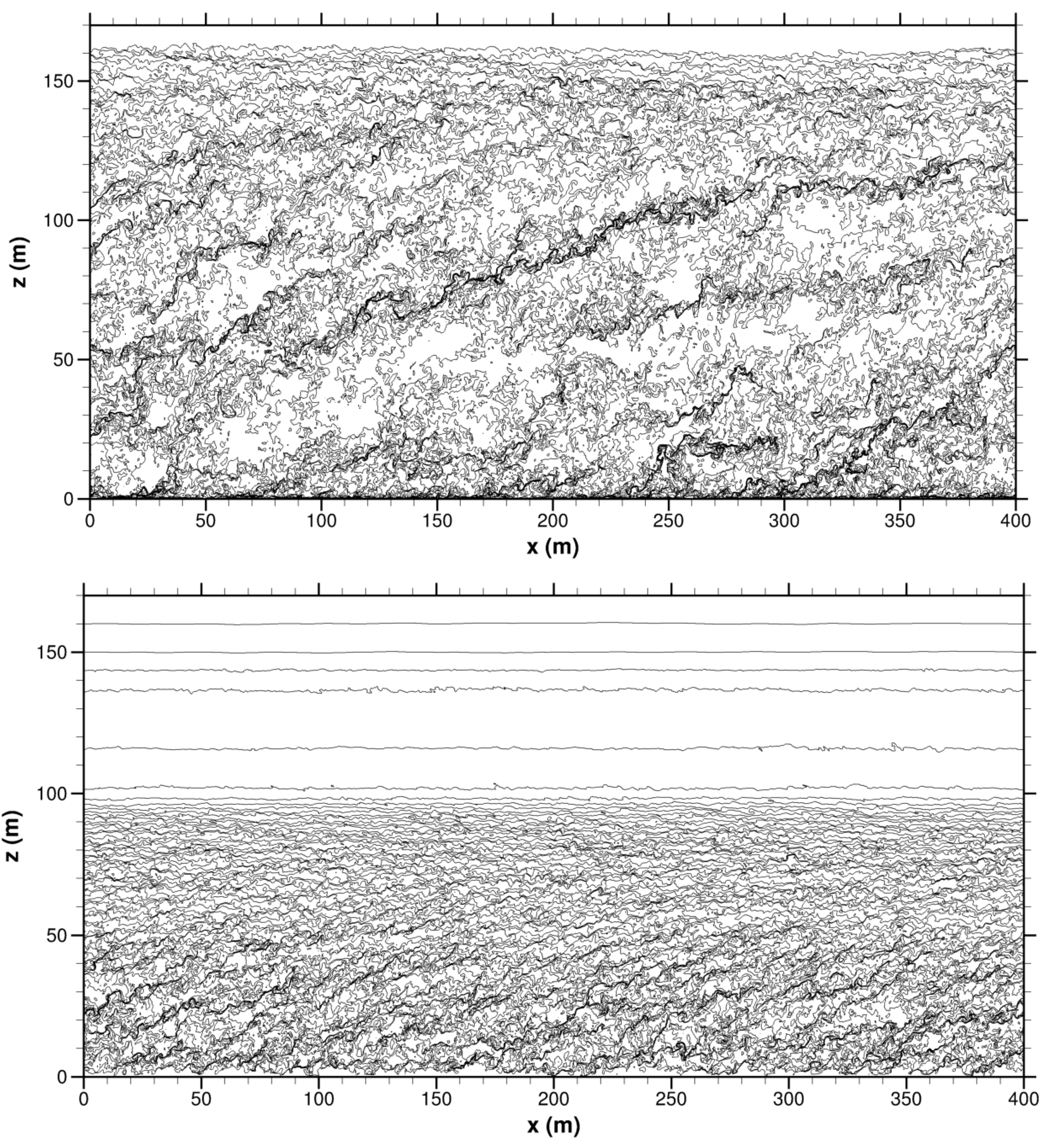
Flow visualization is extensively utilized to identify turbulent structures in the SBL; an example is provided in
Figure 7. This image shows the instantaneous temperature isolines in an
plane from simulations C2 and F2 with weak and strong stratification, respectively. Inspection of the images shows an abundance of tightly compressed contour lines sprinkled throughout the SBL; the sharp gradients in
are signatures of warm–cold temperature fronts passing through the domain. Notice that the temperature fronts are very sharp and tilted in the downstream direction, primarily a consequence of the sheared streamwise velocity
. Animations show the spatial and temporal evolution of the fronts (not shown). Frequently, the fronts are observed to extend over the full depth of the SBL and nearly the full horizontal extent of the domain, as shown in the upper panel of
Figure 7. Turbulent mixing between fronts at different
z levels leaves voids with nearly constant temperatures. Thus, at a fixed
location a vertical profile of
displays a staircase pattern as different front families are crossed. As the stratification increases, the fronts tilt farther downstream and the separation between fronts shrinks considerably, as shown in the lower panel of
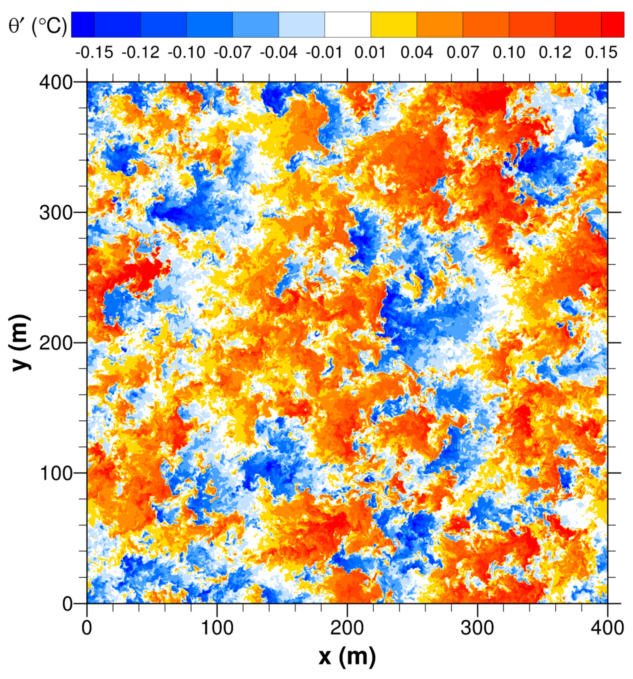
Figure 7. A horizontal slice through the domain at
m from simulation C2 provides a sense of the front coherence in the spanwise direction as well as the spatial randomness of the fronts.
Figure 8 shows multiple fronts at various positions in the horizontal domain; the spanwise extent of a front is ∼50 m or less. At this instance in the simulation the warm upstream side of the front is modestly stronger than the cool downstream side of the front.
Figure 7.
Temperature isolines in an plane from simulations with weak surface cooling (C2 upper panel) and strong surface cooling (F2 lower panel) at h, respectively. In the upper panel there are 51 contour levels between C. In the lower panel there are 71 contour levels between C. In addition, in the lower panel, contour levels C are shown for m. The reference temperature K.
Linear stochastic estimation (LSE) pioneered by Adrian [
56] is used to compute the conditional averages of the turbulent fields in the SBL. Our application of LSE [
20] uses an event trigger based on a positive–negative temperature jump separated by a finite distance in a horizontal plane. This event choice is guided by the instantaneous flow visualization of
shown in
Figure 8, which depicts numerous warm–cool temperature fronts. As an example, our LSE temperature event with
K corresponds to a scalar flux about five times the surface value
. The conditional fields
, velocity gradient tensor
, and vorticity
are estimated for a range of vertical locations, spatial separation, and event amplitudes [
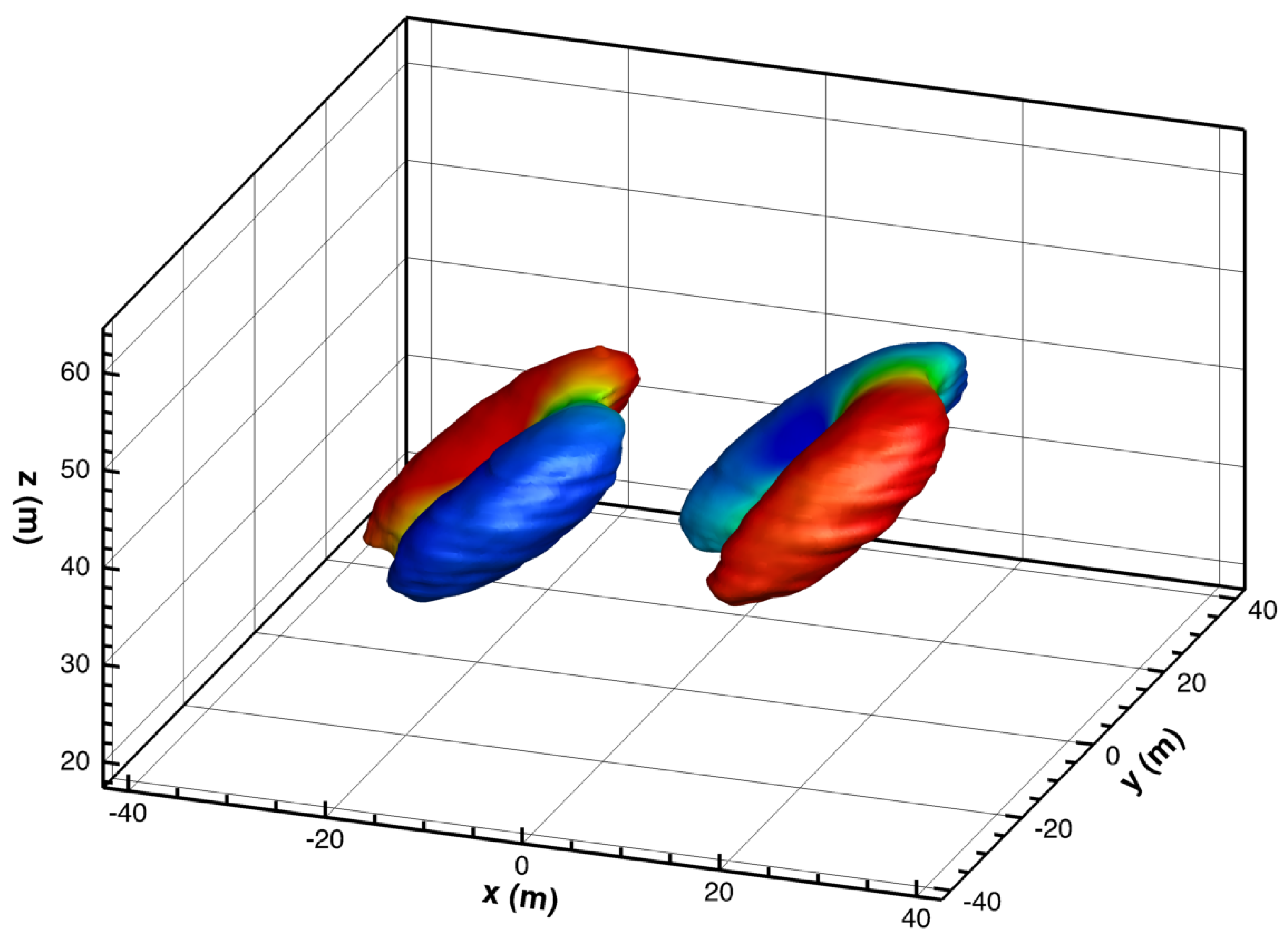
20]. Our conditional sampling finds pairs of counter-rotating vortices in the SBL, as shown in
Figure 9. The vortices are aligned with the mean wind direction and are tilted forward in the downstream direction. The upstream vortices act in concert to pump warm fluid forward while the downstream vortices pump cool fluid backwards, resulting in a near-stagnation point in the region between the vortices. The front boundary is very sharp but the vortices creating the fronts are well-resolved coherent structures. Sullivan et al. [
20] show that the scale of the vortices lies near the peak in the spectrum for
and
w. The coherent structures in the interior of a sheared SBL are considerably different than the pancake vortices in large-scale stably stratified turbulence away from a boundary [
57].
Figure 8.
Fluctuating temperature field at from simulation C2 at h. Examples of sharp warm–cold temperature fronts are located at = (20, 230), (200, 270), (230, 50), (230, 220), (330, 340) m. The color bar for is in units of °C.
Figure 8.
Fluctuating temperature field at from simulation C2 at h. Examples of sharp warm–cold temperature fronts are located at = (20, 230), (200, 270), (230, 50), (230, 220), (330, 340) m. The color bar for is in units of °C.
5.3. SFS Motions in Observations and LES
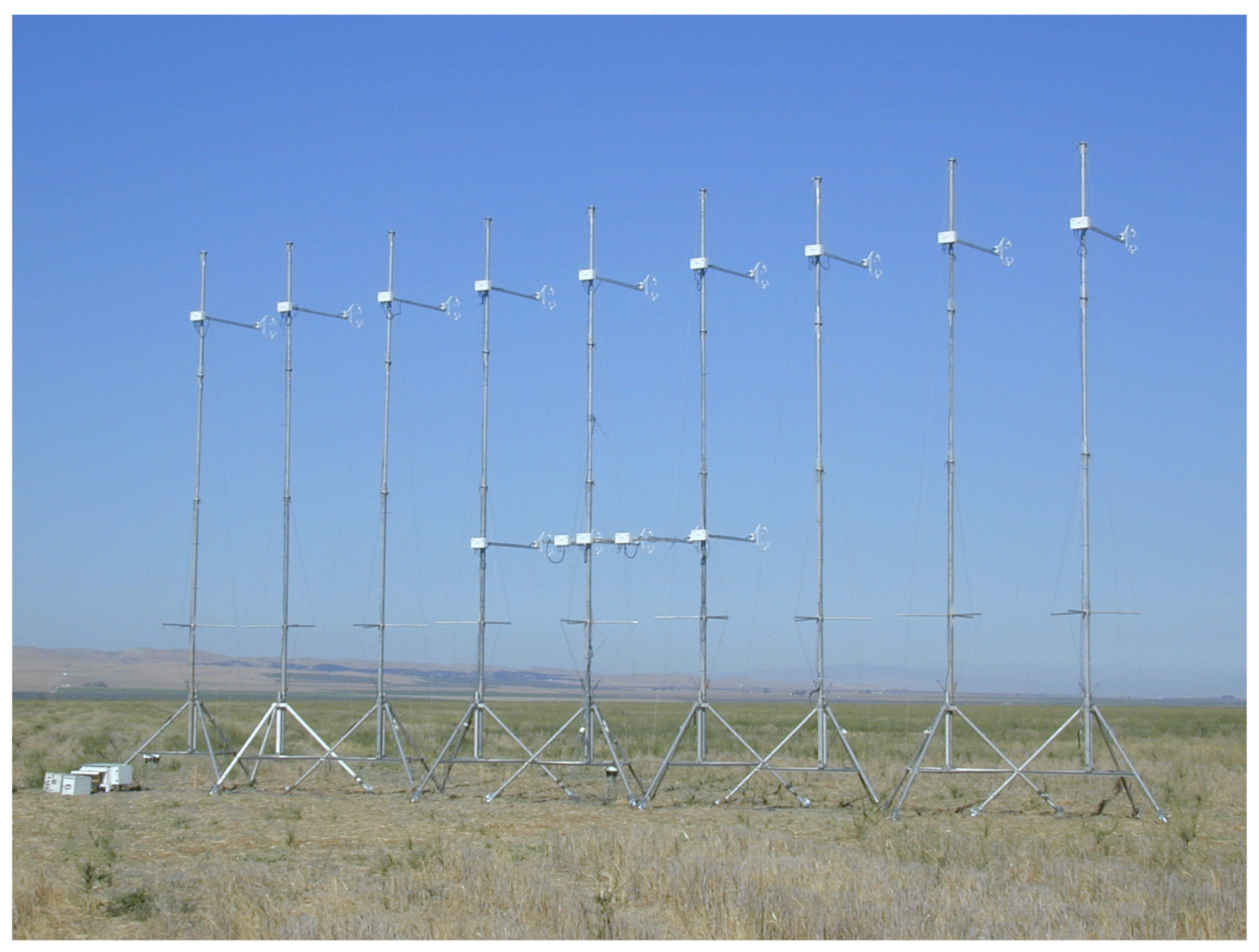
The HATS dataset contains a mix of variations in wind speed, stratification, and perturbations in the array configuration, i.e., the vertical location
and horizontal separation
of the anemometers shown in
Figure 1. To account for these variations in computing the SFS motions Sullivan et al. [
37] introduced a resolution ratio
. The filter scale
and is isotropic in
; only 2D filtering is employed in HATS. The vertical velocity is used to define
for the following reasons:
w is the least-resolved field in LES,
w statistics closely follow Monin–Obukhov similarity relationships in the surface layer, and
w impacts the vertical fluxes, which are key ingredients in LES and also large-scale models. The length scale
where
is the mean wind speed and
is the Eulerian integral time scale for vertical velocity. The autocorrelation function for
w is fit to the form
. This equates to finding a spectral peak in the vertical velocity spectrum assuming a high wavenumber spectrum
; see Kaimal and Finnigan [
58] (p. 63), Sullivan et al. [
37], and Horst et al. [
30]. This definition of
is robust and accounts for the distance
z above the surface and stratification. In HATS the resolution ratio spans the range
.
Figure 9.
Oblique view of the typical 3D vortical structures in the SBL at a height
from simulation C with grid mesh of 1024
points [
20] obtained using linear stochastic estimation-based conditional averaging. To indicate the sign of vortical rotation, the surface is colored by the vertical component of the vorticity vector
with deep red (blue) colors corresponding to positive–upward (negative–downward) rotation, respectively. The mean horizontal winds are from left to right and at this height turn 30.6 degrees towards the
direction.
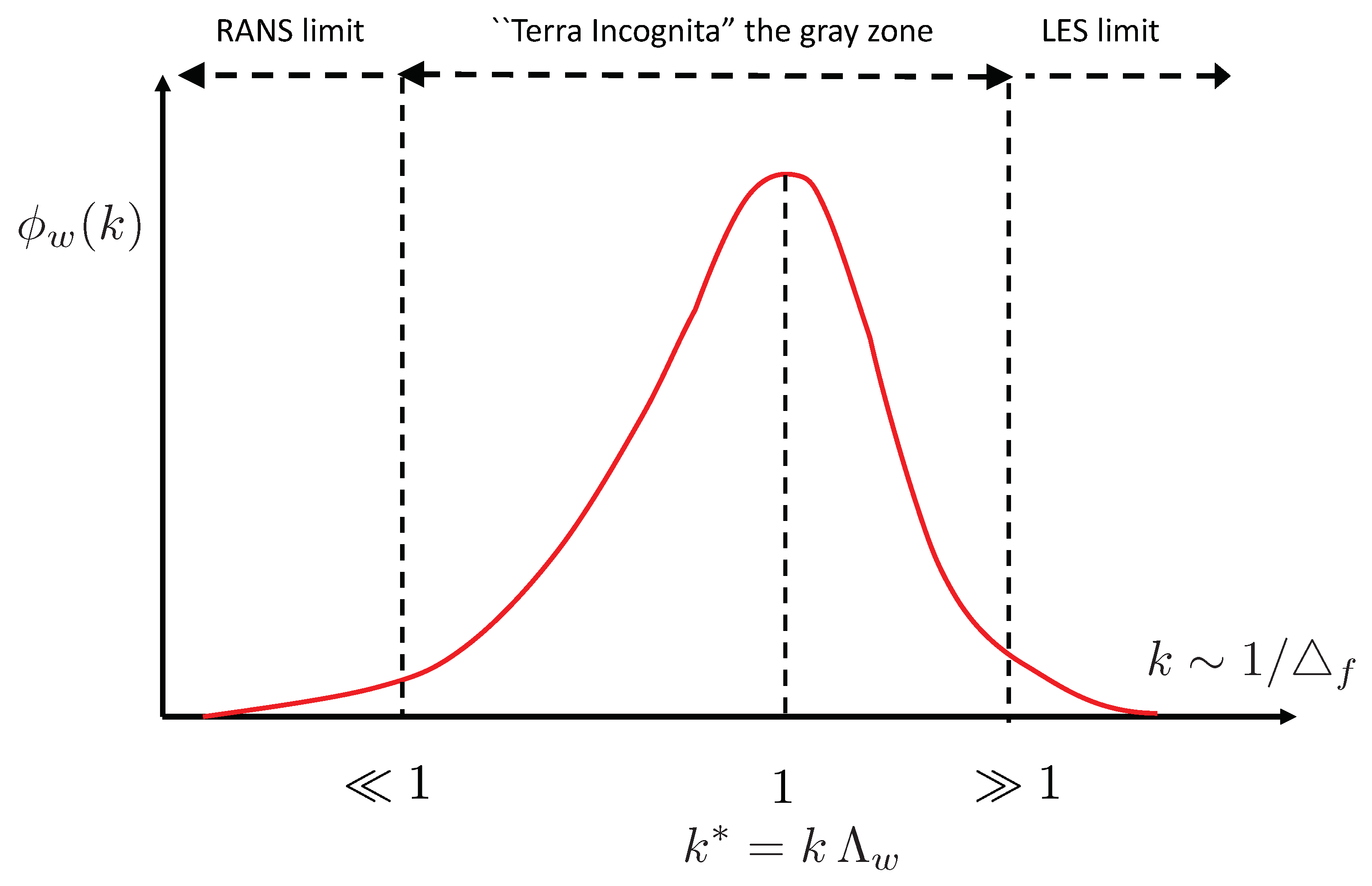
Physically,
is a measure of the scale separation between the large-scale energy-containing eddies and eddies near the filter scale, as sketched in
Figure 10. For
the separation is wide and the turbulence is well-resolved with the filter scale in the inertial range. Meanwhile, for
, the filter scale is near or left of the energy-containing eddies and the energy-containing turbulence is thus under-resolved. The ratio
is a measure of the simulation resolving power. When
the simulation is LES and when
the simulation is akin to unsteady Reynolds-Averaged Navier–Stokes (RANS). Wyngaard [
40] calls the intermediate regime
“Terra Incognita”, which has similarity with the so-called gray zone [
59,
60]; it is unknown if the SFS closures used in LES or RANS are applicable in the gray zone. As
varies between the LES and RANS limits the length scale
ℓ in an eddy-viscosity closure is predicted to vary linearly with the grid spacing
until ▵ exceeds the scale of the energy-containing eddies
, then
ℓ becomes constant [
61]. The crossover from LES to RANS is also recognized in the engineering community: Perot and Gadebusch [
62] describe a two-equation self-adapting closure that spans the regime from DNS to LES to RANS for a mixing layer. Our estimate of a scale-aware length scale for dissipation in the SBL is discussed below.
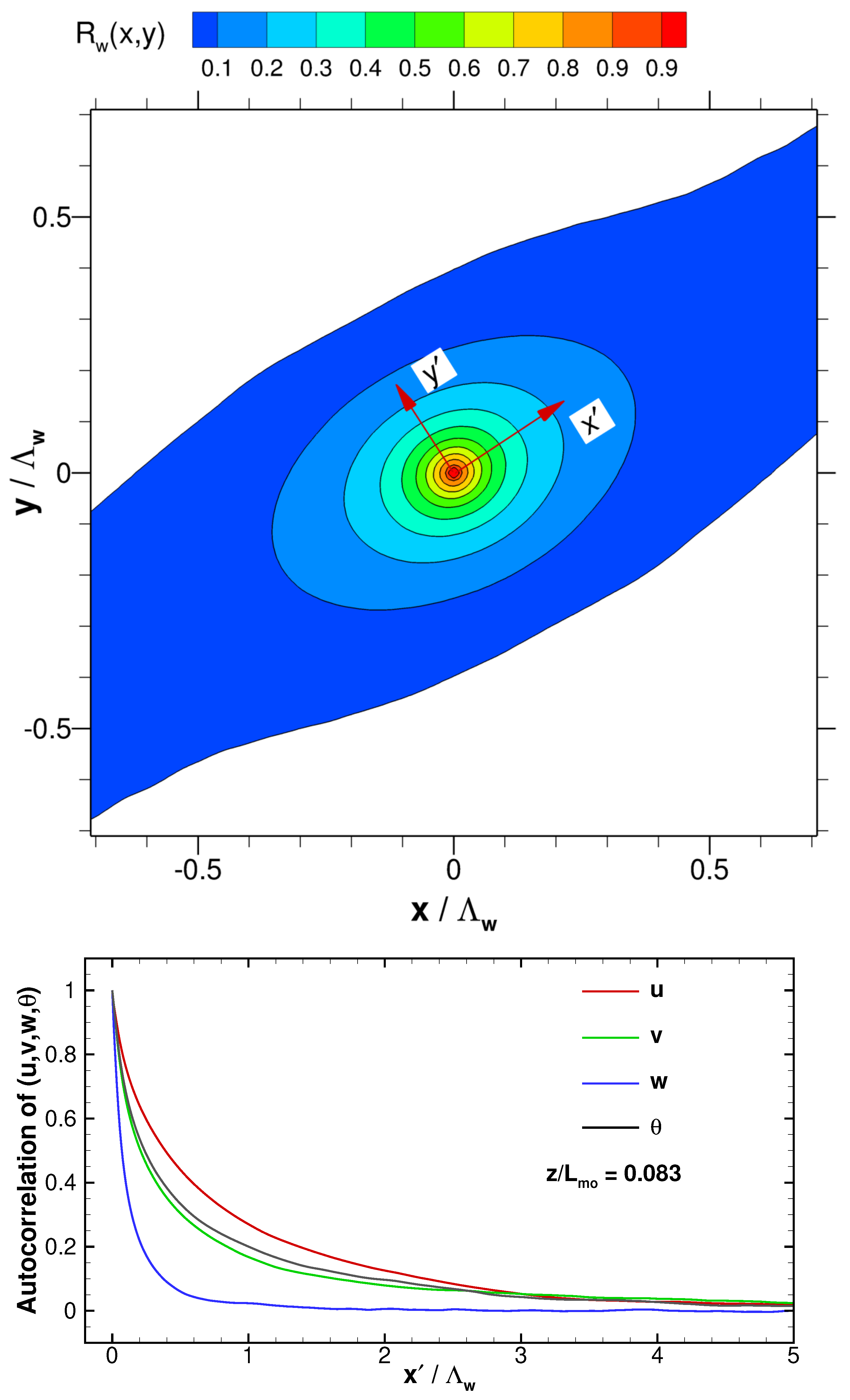
To make a quantitative comparison between HATS and LES, we define the LES length scale
in terms of the spatial autocorrelation of vertical velocity
, but aligned with the mean wind direction (see
Figure 11). For LES,
, where
is the integral scale obtained by integration of the autocorrelation
from
to its first-zero crossing; Taylor’s hypothesis is not used. The resolved fields
, used to compute SFS motions, are also rotated into the mean-wind coordinate frame
.
Figure 10.
A sketch of the vertical velocity spectrum
in a horizontal plane as function of the horizontal wavenumber magnitude
k. Its peak is at the non-dimensional wavenumber
. The limits
and
are the LES and RANS regimes, respectively. In between these two limits is “Terra Incognita” or the gray zone. Figure is adapted from Wyngaard [
40].
Analysis of the LES fields uses a filter scale
referenced to the scale
used in its subgrid model. For simulation C2 with the 2048
mesh and uniform spacing in all three directions the length scale in the subgrid model is
=
▵ = 0.25 m. Filter scales in the range
are used in the present analysis. The lower limit is chosen to help minimize contamination from the subgrid model while the upper limit is constrained by the horizontal dimensions of the LES box, 400 m in each direction. The turbulent fields at vertical levels
inside and near the top of the surface layer are analyzed; at these two levels
m. Thus, the resolution ratio possible with the LES data spans
, which nicely overlaps with the HATS data. The spatial filtering is a simple top-hat filter applied sequentially in the
directions, and the results from ten volumes are averaged to construct the SFS statistics. The SFS momentum and temperature fluxes, in both observations and LES, are constructed from:
where the overhat notation
denotes two-dimensional
spatial filtering at
.
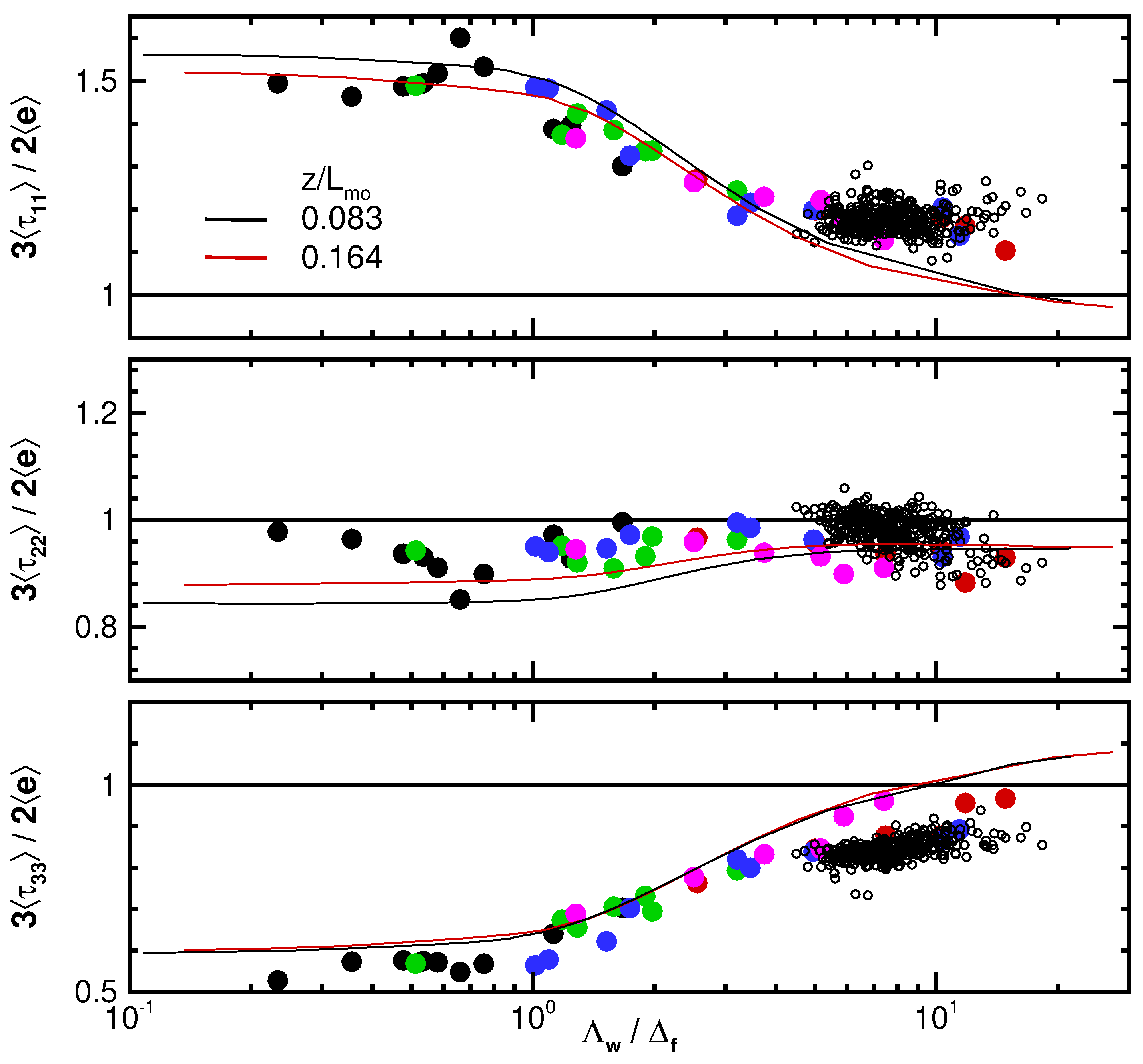
The variation in the SFS velocity variances
, momentum fluxes
, and temperature fluxes
with varying resolution ratio
from HATS, OHATS, and LES are shown in
Figure 12,
Figure 13 and
Figure 14, respectively. Because of physical constraints, OHATS employed only a single array with horizontal spacing
m. As a result, the variation in
from OHATS is a consequence of weak diurnal changes and possible wave effects over the ocean. The small value of
pushes all the OHATS results towards large
to 10. HATS employed four different array configurations and, coupled with a vigorous diurnal cycle, results in a wide range of the resolution ratio. Inspection of the HATS data shows stratification is important, as the spectral peak in vertical velocity shifts from large to small scales as the stratification transitions from unstable to stable [
58]. For example, the results from HATS array-1 at
m, blue bullets in
Figure 12, span nearly a decade in
as
(see Sullivan et al. [
37]).
Figure 11.
Two-dimensional autocorrelation for vertical velocity at from simulation C2 at h (upper panel). The 1d correlation, extracted from the 2d correlation, for aligned with the mean wind direction at (lower panel). The peak wavelength for the w correlation is m.
Figure 11.
Two-dimensional autocorrelation for vertical velocity at from simulation C2 at h (upper panel). The 1d correlation, extracted from the 2d correlation, for aligned with the mean wind direction at (lower panel). The peak wavelength for the w correlation is m.
Figure 12.
Variation of subfilter-scale velocity variances with resolution ratio
. Measurements are collected in the atmospheric surface layer over land (colored bullets are from different sonic arrays in HATS) and over the ocean (open circles from OHATS) [
37,
47]. The (red, black) lines are filtered results from simulation C2 with mesh 2048
. The (red, black) lines are in the surface layer
, respectively. The measurements and simulation results highlight the deviation from isotropy when the resolution ratio is
.
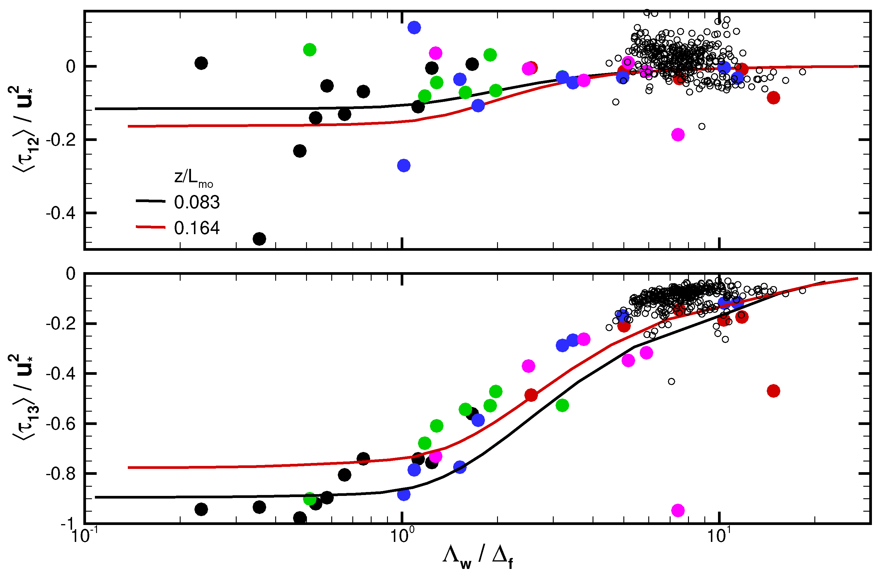
Overall, the qualitative agreement between the simulation results and observations for variances and fluxes is good, and in some instances the comparison is quantitatively good. The normal variances
in
Figure 12 are essentially a bulk metric of SFS isotropy. The observations and simulations both show that the variances
tend to unity only for large
; isotropy at small scales is an implicit assumption in most Smagorinsky closures for LES, and thus fine computational grids are apparently needed to satisfy this metric. For
the ratio
indicates high anisotropy in the peak energy-containing eddies in the streamwise and vertical components. The momentum fluxes
computed from LES fields are in good agreement with the observations. Notice the vertical momentum flux shows an expected steady approach towards
at small
at the level
. The results also suggest that the
level is slightly outside the surface layer in the SBL. At small values of
, the LES results show a departure of the horizontal variance
from isotropy, qualitatively consistent with the measurements but perhaps to a somewhat greater degree. The LES also shows non-zero values of horizontal momentum flux
, while the measurement scatter is too great to confidently assess this.
Figure 13.
Variation of subfilter-scale momentum fluxes with varying resolution ratio
. Horizontal momentum flux
(
upper panel) and vertical momentum flux
(
lower panel). Measurements are collected in the atmospheric surface layer over land (colored bullets) and ocean (open circles) [
37,
47]. The (red, black) lines show filtered results from simulation C2 with mesh 2048
and spacing
m. The (red, black) lines are in the surface layer
, respectively. Note the different vertical scale in the upper and lower panels.
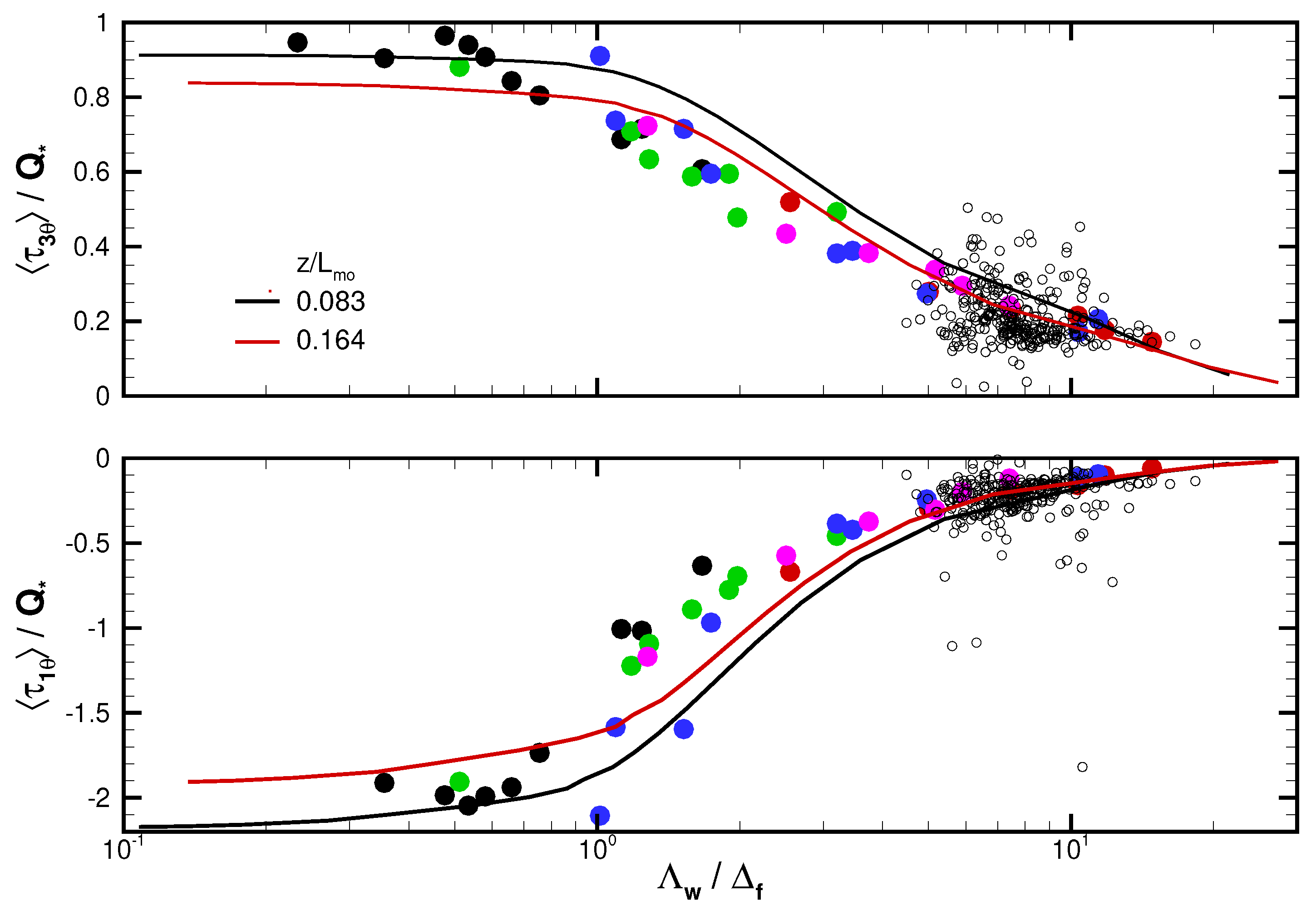
Figure 14.
Variation of subfilter-scale temperature fluxes with varying resolution ratio
. Horizontal flux
(
upper panel) and vertical flux
(
lower panel). Measurements are collected in the atmospheric surface layer over land (colored bullets) and over the ocean (open circles) [
37,
47]. The (red, black) lines show the filtered results from simulation C2 with mesh 2048
. The (red, black) lines are in the surface layer
, respectively.
The horizontal and vertical scalar fluxes
are interesting. These SFS fluxes from LES are in good agreement with the observations. Notice as
the vertical scalar flux tends to the surface flux
as expected while the horizontal scalar flux tends to −2.5, which agrees very well with the HATS observations and also with the classic Kansas results, where Wyngaard et al. [
63] find the ensemble average of the total scalar flux
at large positive values of the stability parameter
. Based on the equations for scalar flux, Wyngaard [
61] points out that
is produced by tilting of the vertical scalar flux by vertical shear
, not by a horizontal gradient
, i.e., an eddy viscosity model is inadequate for horizontal scalar flux when
is small. Dynamically, the tilted vortices in
Figure 9 are the agent producing horizontal scalar flux, as discussed in [
20].
The average SFS variances and fluxes from LES agree well with the HATS and OHATS observations over a wide range of
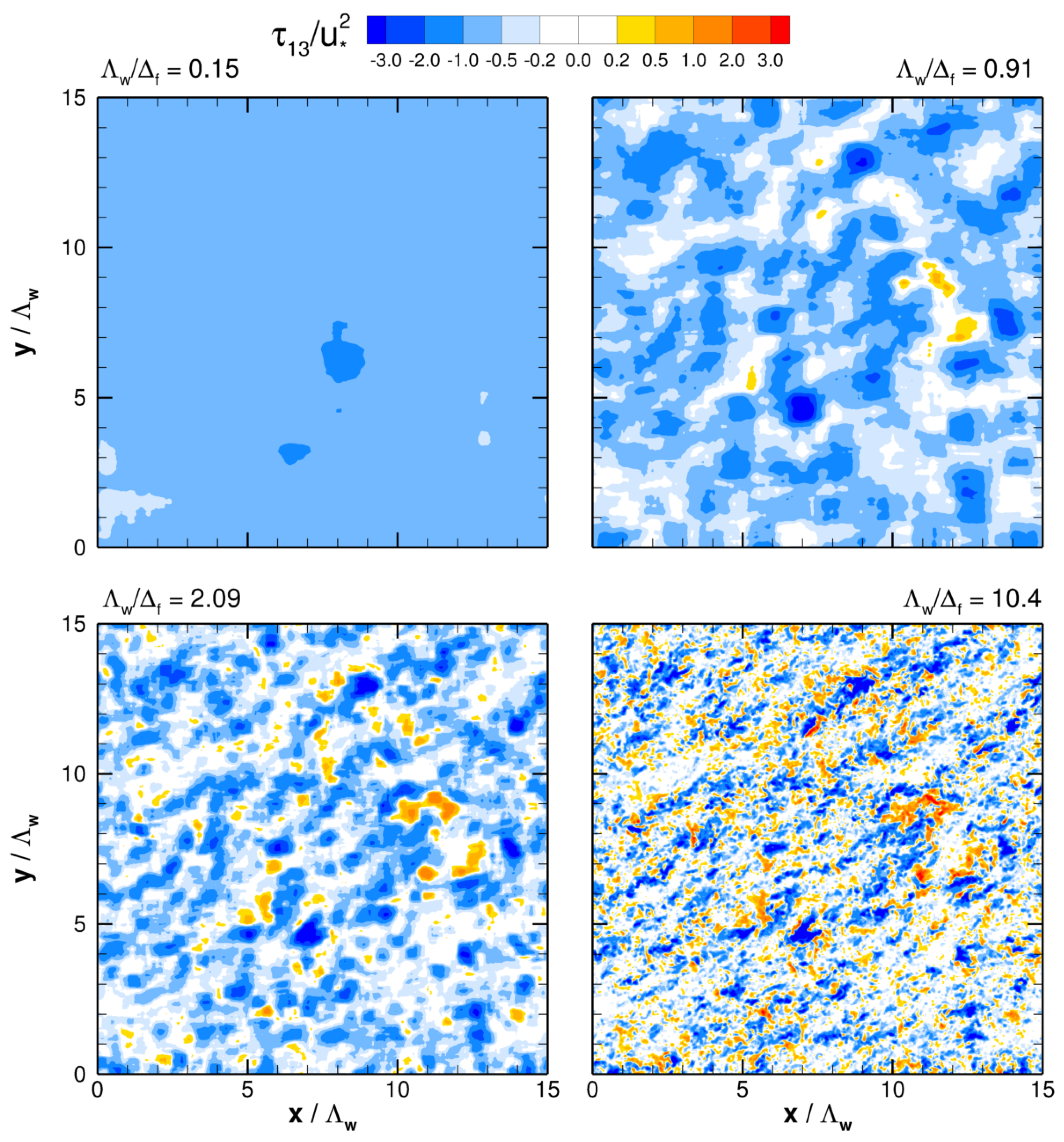
, and thus we expect the instantaneous spatially varying SFS motions from LES are also representative of atmospheric surface-layer flows. The visualizations in
Figure 15,
Figure 16 and
Figure 17 show the vertical momentum flux and vertical and horizontal temperature flux in the horizontal planes at level
m for resolution ratios
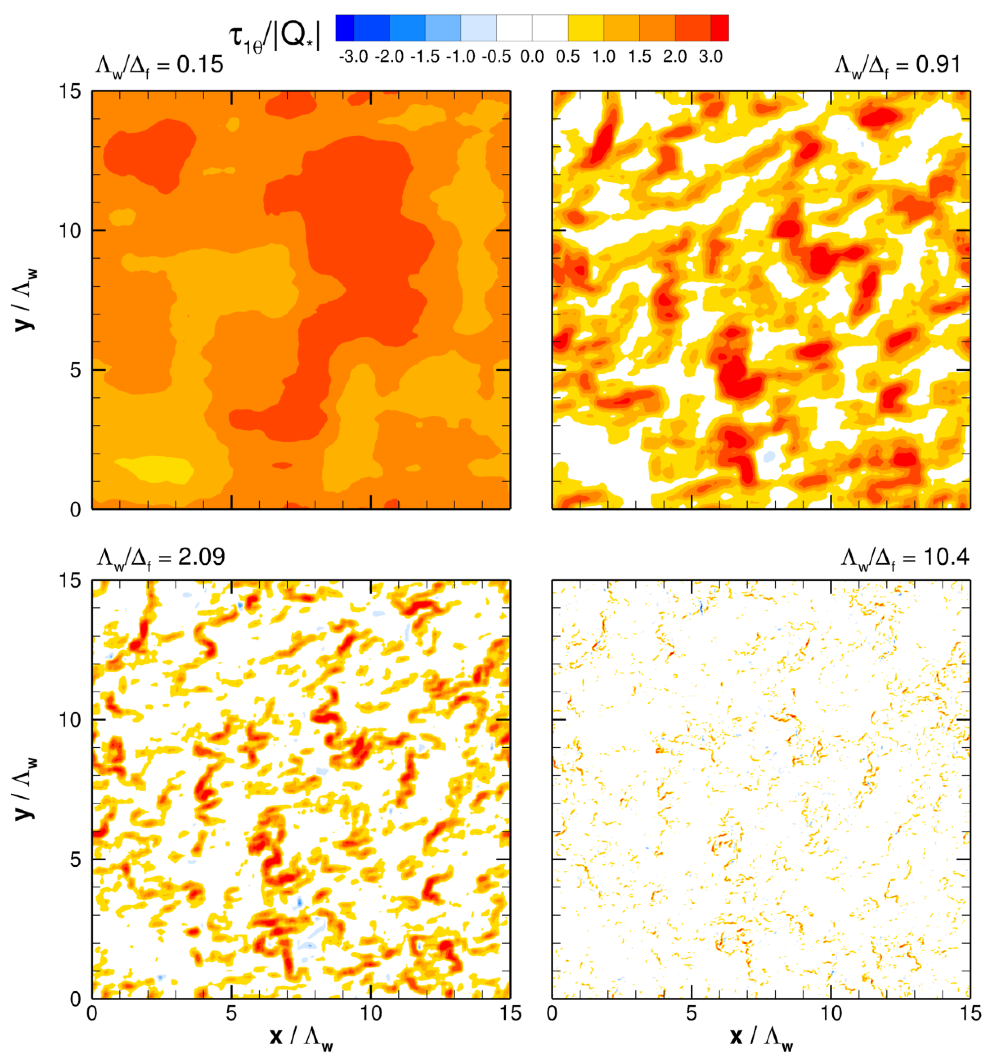
, i.e., spanning either side of the gray zone. Inspection of the figures shows a smooth transition with varying
. A parameterization needs to model all of the flux when
is small and stochastic fluctuations at large
. In the intermediate gray zone the SFS motions contain a fraction of the total flux (see
Figure 13), but stochastic fluctuations are also clearly present at the same time, e.g., see the visualization in
Figure 15.
Figure 15.
Subfilter-scale momentum flux at m with varying resolution ratio from simulation C2. The normalization is by .
Figure 15.
Subfilter-scale momentum flux at m with varying resolution ratio from simulation C2. The normalization is by .
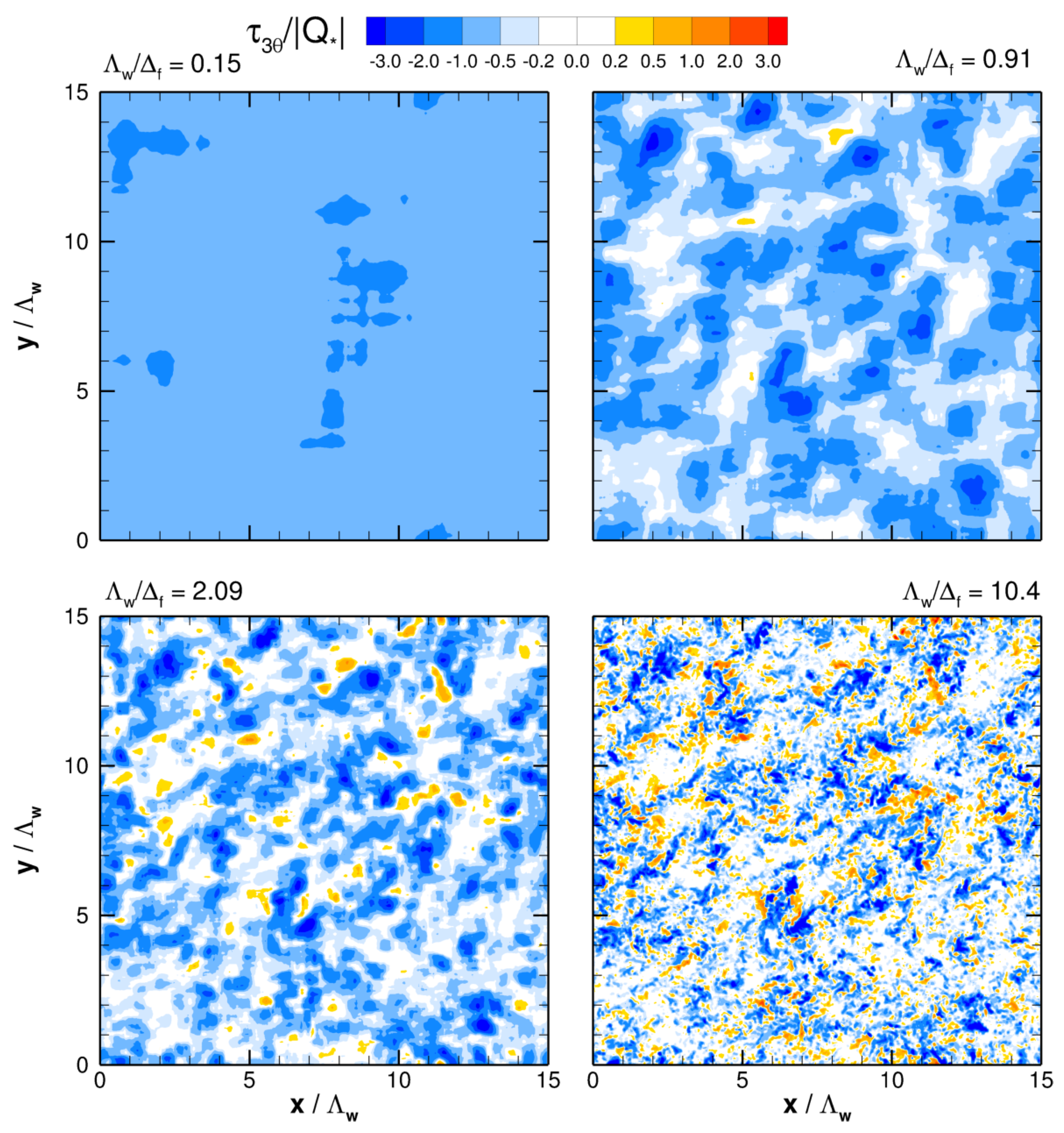
Figure 16.
Subfilter-scale vertical temperature flux at with varying resolution ratio from simulation C2. To preserve the sign of the flux the normalization is by .
Figure 16.
Subfilter-scale vertical temperature flux at with varying resolution ratio from simulation C2. To preserve the sign of the flux the normalization is by .
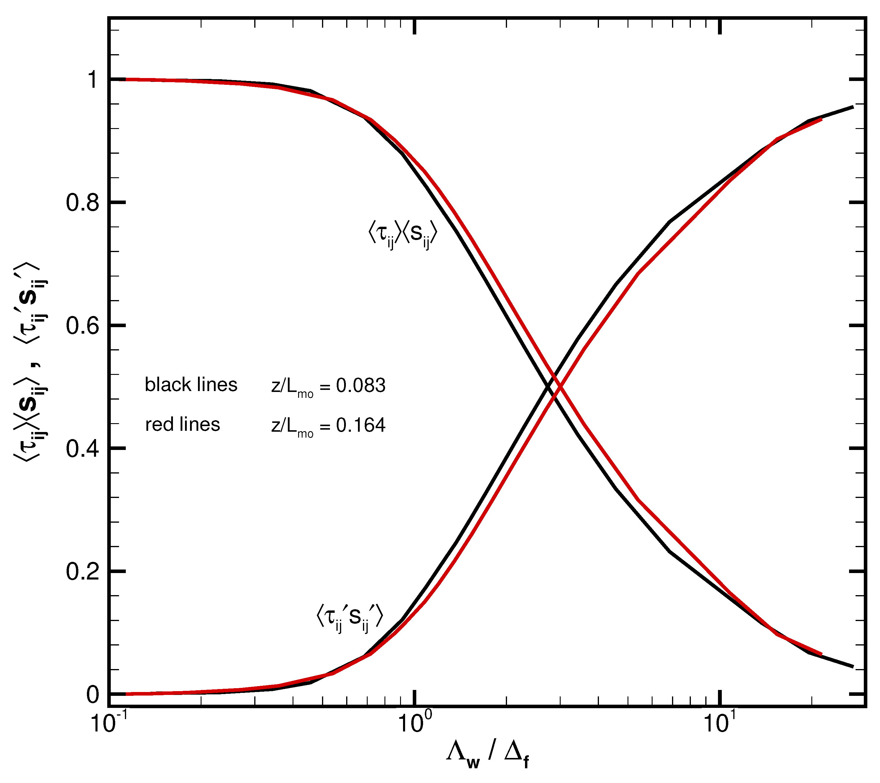
In the gray zone, to ensure the proper energy transfer between the resolved and subgrid fields, a SFS flux parameterization needs to account for a fraction of the net flux plus fluctuations correlated with the fluctuating strain rate. To illustrate the idea, consider the energy equation for the resolved motions, which contains the transfer term
, where
is the resolved rate of strain tensor; recall this term also appears in the SFS energy equation with opposite sign [
64]. Decomposing the SFS flux and resolved rate of strain tensors into a mean and fluctuation yields the expression
notice that
allows both forward and backward (backscatter) motion of energy, which was observed in HATS [
37]. Inspection of (5) shows the difficulty: energy transfer at small and large
is
or the turbulent correlation
, respectively. However,
Figure 18 shows that in the intermediate gray zone both terms on the right-hand side of (5) contribute to the energy transfer. Thus, a SFS flux parameterization needs to account for a fraction of the net flux but also important stochastic fluctuations because of the energy transfer between the resolved and subgrid fields. The SFS momentum fluctuations are not random noise but are clearly correlated with fluctuations in the strain rate. The transfer of scalar variance faces a similar dilemma in the gray zone.
Figure 17.
Subfilter-scale horizontal temperature flux at with varying resolution ratio from simulation C2. To preserve the sign of the flux the normalization is by .
Figure 17.
Subfilter-scale horizontal temperature flux at with varying resolution ratio from simulation C2. To preserve the sign of the flux the normalization is by .
Parameterizations in the gray zone are further confronted by the possible “double counting” of the momentum and temperature fluxes. This can result when a SFS paramterization is used outside its design range in the space
. For example, this can occur in the gray zone
when a single-column model, designed for RANS vertical flux, is used at the same time the model grid resolution is sufficient to support the resolved turbulence. Under these conditions the estimate of flux can be double counted [
60]. Flux double counting spoils the energy and scalar transfer between the resolved and SFS fields.
A cursory inspection of the patterns in
(
Figure 15) and
(
Figure 16) suggests a possible amplitude correlation, i.e.,
is approximately related to
by a constant [
65]. The assumption that the scalar diffusivity and momentum eddy viscosity are related is routinely adopted by LES models. The visualization of the streamwise scalar flux shows a near-zero mean and small fluctuations at large
;
is routinely neglected in SFS modeling [
66]. At small
the horizontal scalar flux is clearly non-zero, but its impact disappears under the usual assumption of a periodic horizontally homogeneous flow
.
Figure 18.
Variation of the production terms in Equation (5) for varying filter width at two heights near the surface denoted by (black, red) lines, respectively, from simulation C2. The individual production terms are normalized by the total production at each filter width. Total production is nearly constant with varying , but slopes downward at small filter widths because of the actual subgrid model used in the LES.
The fine-mesh LES results can also be used to craft parameterizations that span the gray zone. For example, consider a
second-order closure that uses a prognostic equation for the unresolved SFS turbulence kinetic energy
with
ℓ a prescribed length scale. This closure uses a TKE equation with a model for viscous dissipation
[
65], typically of the form
The dissipation model requires specification of the length scale
.
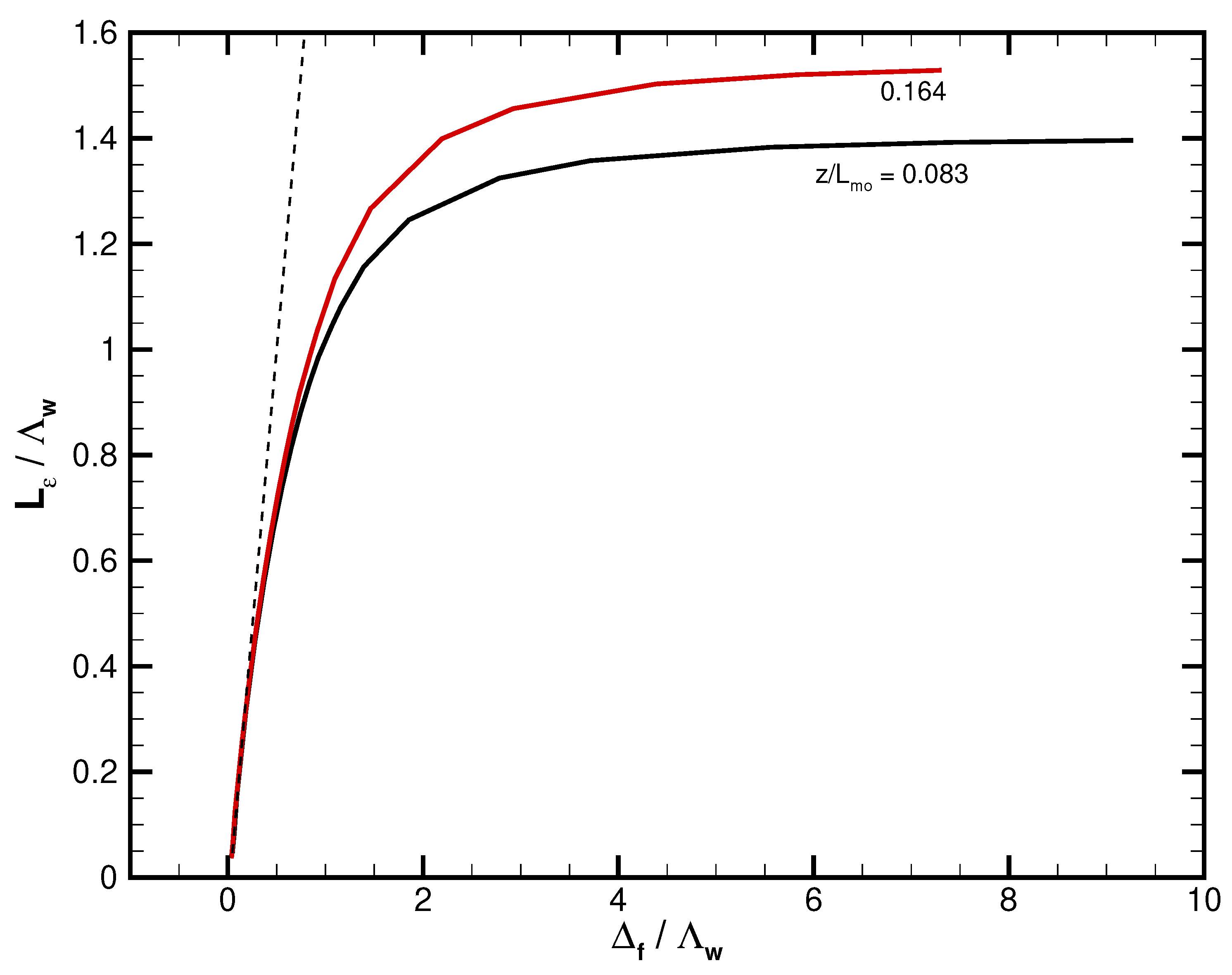
Figure 19 shows the variation of
with inverse resolution ratio
computed from the LES results; this result is obtained by assuming a constant dissipation across
. For small filter widths in the LES regime,
is a small fraction of the total energy and
. At large filter widths approaching the RANS regime,
is the total kinetic energy and the length scale saturates, i.e.,
in the surface layer. A smooth variation of
is found at intermediate filter widths between the RANS and LES limits. In the middle of the gray zone
at
. Thus, in general one needs an adaptive parameterization
as the filter width varies across the RANS to LES regimes.
Figure 19.
Variation of the dissipation length scale
for varying filter width
at two heights near the surface
denoted by (black, red) lines, respectively, from simulation C2. The black dashed line is a linear fit to
for small filter widths similar to the predictions by Wyngaard [
61].
Figure 19.
Variation of the dissipation length scale
for varying filter width
at two heights near the surface
denoted by (black, red) lines, respectively, from simulation C2. The black dashed line is a linear fit to
for small filter widths similar to the predictions by Wyngaard [
61].


