Article

The Atmospheric Vortex Streets and Their Impact on Precipitation in the Wake of the Tibetan Plateau

1
School of Atmospheric Sciences, Nanjing University, Nanjing 210023, China
2
Jiangsu Collaborative Innovation Center for Climate Change, Nanjing University, Nanjing 210023, China
3
Institute for Climate and Global Change Research, Nanjing University, Nanjing 210023, China
4
Department of Earth, Ocean, and Atmospheric Science, and Center for Ocean-Atmospheric Prediction Studies, Florida State University, Tallahassee, FL 32306, USA
*
Authors to whom correspondence should be addressed.
Atmosphere 2023, 14(7), 1096; https://doi.org/10.3390/atmos14071096
Submission received: 29 May 2023 / Revised: 26 June 2023 / Accepted: 28 June 2023 / Published: 30 June 2023

Abstract

:
Atmospheric vortex streets (AVSs) are often observed in the wake of the leeward side of mountainous islands and are considered atmospheric analogs of the classic Kármán vortex street when a fluid flows past a cylindrical obstacle. The prevailing westerlies were observed year-round around the Tibetan Plateau. However, it remains to be understood whether the wake on the leeward side of the Tibetan Plateau exhibits a stable AVS and how the AVS impacts precipitation over the downstream region. In this study, the environmental meteorological factors, spatiotemporal characteristics, and various properties of the AVS on the leeward side of the Tibetan Plateau were examined for the period of 1979–2018 using global reanalysis datasets. The results show that the spatial structure of these AVSs closely resembles that of the classic Kármán vortex street observed in the laboratory. The meteorological factors satisfy the conditions in which a stable AVS can exist year-round. Moreover, various properties of these AVSs, including the aspect ratio and Strouhal number, are similar to those in previous studies of smaller obstacle caused AVS. Thus, these AVSs on the leeward side of the Tibetan Plateau can be interpreted as the atmospheric analog of classic Kármán vortex streets. The results further show that the spatiotemporal structure of precipitation over the wake of the Tibetan Plateau was largely shared by the cyclonic activities in the AVS. Approximately 80–90% of the total precipitation and heavy rain days in the main rainband over the wake of the Tibetan Plateau are closely tied to the seasonal evolution of the AVS.

1. Introduction

When steady wind flows around an isolated obstacle, such as a mountain or a mountainous island, atmospheric vortex streets (AVSs) can be generated on the leeward side of the obstacle under favorable meteorological conditions. The AVS pattern exhibits a double row of counter-rotating vortex pairs shedding alternately and resembles the classic von Kármán vortex street [1,2,3], as schematically shown in Figure 1. Vortex streets have been frequently observed in the atmosphere [4,5] and ocean [6,7,8,9,10,11]. These types of vortex streets have significant weather and climate implications. Oceanic vortex trains could enhance biological production and turbulent mixing, impacting fishing activities [12,13,14,15]. The atmospheric vortex streets may modulate the cloud and wind patterns over the downstream region [16].
The studies of AVS can be traced back to as early as the 1930s. Lettau [17] suggested that AVSs could be shed by large islands. However, it was not until the early 1960s that researchers observed AVS in cloud images taken by the first generation of earth-orbiting satellites (e.g., [18,19,20]). These studies also revealed the properties of AVS, such as the rate of vortex shedding eddy lifetime, eddy viscosity, and obstacle drag, from satellite imagery and suggested that the AVS on the lee side of obstacles can be interpreted as the atmospheric analog of classic von Kármán vortex streets [18,20,21,22,23,24,25,26]. Further studies analyzed the mechanisms and meteorological conditions under which a stable vortex on the lee side of an obstacle can develop, e.g., Etling [27] conducted laboratory experiments and found that a stable vortex street on the leeward side of an obstacle can exist when the Reynolds number (Re) is larger than a particular value and the Froude number is smaller than 0.4.
In addition to observational and laboratory studies, numerical studies have been carried out to reveal more details of the formation of a vortex pair on the leeward side of the island and its separation from the island. These studies are documented in the review paper of Young and Zawislak [7]. To date, most numerical simulations of Kármán vortex shedding in the real atmosphere have focused on islands in the Northeast Atlantic [5,28,29,30] or in the Northwest Pacific [31]. Based on a numerical simulation model with a horizontal resolution of 2 km, Nunalee and Basu [5] revealed that the whole region in the satellite image with a cellular stratocumulus cloud pattern was disturbed by Kármán vortex shedding. Li et al. [31] simulated the observed AVS using an MM5 model and estimated a vortex-shedding rate of 1 h.
It is noted here that previous observations of AVS, including those mentioned above, focused on AVS at a spatial scale of approximately a few hundred kilometers that can be captured in a non-merged satellite image. For AVS of these spatial scales, the Reynolds number, the ratio of inertial forces to viscous forces within a fluid, is usually between 50 and 500 [25]. From a theoretical perspective, given that the Reynolds number is proportional to the spatial size of the obstacle, a stable vortex street can exist when the Reynolds number is as high as 105 [25,32], as demonstrated in laboratory experiments. However, there have been few observational studies on that scale. It is indeed this hidden possibility that is one of the reasons for us to explore whether the Tibetan Plateau, standing in strong seasonally varying westerlies, can cause AVS of similar spatial scales on its leeward side.
The Tibetan Plateau, located over South-Central Asia, is the world’s highest plateau above sea level, with an average elevation of approximately 4500 m (approximately one-third of the tropospheric height). Prevailing year-round lower tropospheric westerlies flow over or flow around the Tibetan Plateau and are divided into two branches after passing by the Tibetan Plateau [33,34], with the portion of flow around being dominant in the low- to mid-tropospheric region [35,36,37]. Yeh noticed, as early as the 1950s, that a pair of vortices appeared frequently on the east sides of the Tibetan Plateau [33]. The southern vortex is cyclonic and associated with low surface pressure and is termed the southwest China vortex [38]. The downstream propagation of southwest China vortices can result in substantial precipitation in downstream regions [39,40]. The northern vortex is anticyclonic and called the little northwest high [41]. However, whether the downstream mesoscale vortices are indeed AVS and how they are directly tied to seasonally varying westerlies have not received much attention from researchers.
This study aims to answer the following questions by analyzing high-resolution reanalysis data: (1) Can the mesoscale systems on the leeward side of the Tibetan Plateau be interpreted as the atmospheric analog of classic von Kármán vortex streets? Do the surrounding meteorological factors and properties of the AVS satisfy conditions in which a stable vortex on the lee side of an obstacle can exist? (2) If so, does the AVS on the lee side of the Tibetan Plateau impact the precipitation and heavy rain days over the wake of the Tibetan Plateau?
The paper is organized as follows: Section 2 describes the reanalysis datasets and precipitation data used. Section 3.1 gives an overview of the seasonal variability of the meteorological situation of the Tibetan Plateau and demonstrates whether the meteorological factors satisfy the conditions under which a stable vortex AVS can exist. Section 3.2 demonstrates the similarity between the AVS on the lee side of the Tibetan Plateau and the vortex street recorded in the laboratory experiment. Section 3.3 calculates some AVS properties, such as the aspect ratio and the Strouhal number identified directly from the reanalysis datasets. Section 3.4 reveals the impact of the AVS on precipitation over the wake of the Tibetan Plateau. Finally, Section 4 summarizes our results and discusses the relationship between AVS and the meteorological systems controlling precipitation over the wake of the Tibetan Plateau.

2. Materials and Methods

2.1. Data

Daily and 6-h horizontal winds and air temperature were derived from the reanalysis of the European Center for Medium-Range Weather Forecasts (ECMWF) interim reanalysis (ERA-Interim) products [42], spanning the 40-yr period from 1979 to 2018. The dataset we obtained is a spatially gridded one that has a fixed horizontal resolution of 1° × 1° and 37 vertical levels. Daily and 6-h horizontal winds and air temperature (2.5° × 2.5° and 17 vertical levels) were also obtained from the National Centers for Environmental Prediction and National Center for Atmospheric Research (NCEP/NCAR) [43] for the period of January 1979–December 2018. It is noted that the key results presented later in this paper are not sensitive to the selection of reanalysis datasets. Following Curio et al. [44], the relative vorticity was calculated from the wind field and was employed to represent the vortices. Interpolation methods were used to obtain a spatial resolution of 1° × 1° and a temporal resolution of 1 h, if necessary.
The daily precipitation in East Asia for the period of 1 January 1979 to 31 December 2018 was obtained from the CPC precipitation dataset [45]. We selected this period to match the duration of the ERA-Interim and NCEP/NCAR datasets. The APHRO_MA_025deg_V1003R1 product based on the APHRODITE rain gauge data precipitation dataset for the 1979–2015 period was also used in this study [46]. Both precipitation datasets have a fixed horizontal resolution of 0.5° × 0.5°. In the following section, we will demonstrate that the results relevant to precipitation are not sensitive to the selection of the precipitation datasets.

2.2. Spatial Fourier Transform to Derive the AVS Pattern

The relative vorticity and horizontal wind field were divided into the AVS-related component and other wave-related components using the Fourier transform, which has been widely applied in wave analysis [47,48]. In this study, the spatial lowpass filtered relative vorticity captured the AVS related to the Tibetan Plateau. The spatial domain was 60° E–120° W, 10° S–80° N. The components with a meridional wavelength shorter than 7–9° and a zonal wavelength shorter than 14–18° were filtered out. We chose these thresholds due to the distances between neighboring vortices in the AVS being longer than these wavelength thresholds.

2.3. The AVS-Related Precipitation and Heavy Rain Days

Mesoscale cyclonic activities could trigger substantial precipitation. Previous studies have attempted to determine the precipitation associated with mesoscale cyclonic activities. Some studies use a fixed-radius scheme to identify the precipitation related to mesoscale cyclonic activities [44,49]. However, other studies use the outermost closed contour (OCC) to detect the affected precipitation [50]. The domain of mesoscale cyclonic activities is naturally defined by the region covered by the outermost closed contour (OCC) in the potential height or relative vorticity fields. In addition, the precipitation within the coverage of the OCC is defined as related to mesoscale cyclonic activities.
To determine the precipitation associated with the AVS, in this study, following Hanley and Caballero [50], we used the region covered by the OCC instead of a fixed radius to detect the precipitation affected by cyclonic activities in the AVS. The OCC of the AVS was defined as the contour where the spatial Fourier-filtered relative vorticity was zero. The AVS-related precipitation was determined over 110–120° E, 125–130° E, and 130–145° E, respectively. These three regions represent East China, the Korean Peninsula, and Japan, respectively.

3. Results

3.1. Topography of the Tibetan Plateau and Surrounding Meteorological Conditions

The Tibetan Plateau spans the region of approximately 26~40° N, 73~105° E. The grid of (40° E, 32° N) is located upstream of the Tibetan Plateau with an elevation of only 500 m and serves as a reference coordinate grid for the Tibetan Plateau. Figure 2 displays the mean seasonal cycle of the zonal wind at that grid. Strong westerlies prevail over the upstream region and over almost the whole troposphere from 1000 hPa to 100 hPa for a whole year. The minima of the westerlies occurred over the boreal summer.
To determine whether meteorological conditions around the Tibetan Plateau favor the generation of vortex street shedding, two dimensionless indices were employed here to measure the basic flow parameters: the Froude number (Fr) and Reynolds number (Re). Etling [27] showed that a stable vortex street on the lee side of an obstacle can exist when the Froude number (Fr) is smaller than 0.4 and the Reynolds number (Re) falls in a particular range. The particular range of Reynolds numbers (Re) for the generation of vortex street shedding was suggested to be 50–105 for different horizontal sizes of the obstacle [25].
The Froude number is the dimensionless ratio of flow inertia to gravitational forces. The parameter is relevant in the description of stratified atmospheric flows. Here, we calculate the streamlines of the air parcels that flow over and around the obstacle separately [51]. The flow below the level of the partitioning streamline, referred to as dividing streamline height, is regarded as a quasi-2D streamline in horizontal planes.
When the vertical profile of wind speed and stratification is given, the dividing streamline height hc can be calculated based on an implicit expression derived by Snyder et al. [51]:
0.5 U 2 h c = h c h m N 2 ( z ) ( h m z ) d z
where U(z) is the vertical profile of upstream wind speed, hm is the average height of the Tibetan Plateau that is felt by the large-scale flow (average height of Tibetan Plateau plus its boundary layer depth), which is approximately 5000 m, and N(z) is the Brunt-Väisälä frequency. The dividing streamline height hc is then used to calculate the Froude number in the slowly varying (approximated as constant) upstream velocity and stratification [27]:
F r = 1 h c h m
Note that this equation of Fr is different from its glossary definition; this equation of Fr is derived based on laboratory experiments [51] and was recommended to calculate Fr in the real atmosphere [27]. Figure 3 plots the climatological mean of the dividing streamline height hc for various seasons. The dividing streamline height hc falls in the range of 3500 m to 4000 m (approximately 600–700 hPa), indicating that the Froude number varies from 0.2 to 0.3 and falls in the range of Froude numbers that could support vortex shedding year-round. The value of dividing streamline height coincides well with the results revealed by numerical experiments, which illustrates that the westerly flowing around the Tibetan Plateau dominates the flowing over in the middle-low troposphere [52]. At the dividing streamline height level, the diameter of the Tibetan Plateau is approximately 1000 km year-round. The upstream velocity for the Tibetan Plateau at that level is observed to be approximately 8 m/s in summer and 15 m/s in other seasons.
Using the above values, we can estimate the Reynolds number, the dimensionless ratio of inertial force to viscous force, for various seasons. The Reynolds number is defined as:
R e = U o d υ
where Uo is the upstream velocity, d is the obstacle (cylinder) diameter, and ν is the kinematic viscosity of the fluid. A value of ν = 1000 m2/s was used in this study, as suggested by Thomson et al. [25]. The estimated Re is approximately 1.5 × 10⁴ in winter and 0.8 × 10⁴ in summer. The estimated Re is below the upper threshold (105) at which the vortex street with a predominant frequency can exist, suggesting that the Reynolds number falls in the range of Reynolds numbers that could support vortex shedding year-round.

3.2. Characteristics of the AVS on the Leeward Side of the Tibetan Plateau

The analysis in Section 3.1 revealed that the meteorological conditions around the Tibetan Plateau are favorable for the generation of vortex street shedding year-round. What are the characteristics of the AVS on the leeward side of the Tibetan Plateau? In this study, the focus is placed on the downstream AVS, far beyond the sharp downhill region.
To answer this question, in Figure 4a–d, we display four cases of the spatial structure of the Fourier-filtered relative vorticity and horizontal wind over the leeward side of the Tibetan Plateau. These four cases are displayed for the spring, summer, autumn, and winter seasons. Clearly, the Fourier-filtered relative vorticity fields in various seasons all bear close resemblance to that of the classic von Kármán vortex-street patterns observed in laboratory flow experiments and illustrated in Figure 1. The double row of counter-rotating vortex pairs appears on the leeward side of the Tibetan Plateau, confirming a well-defined AVS pattern related to the Tibetan Plateau. The cyclonic vortices and anticyclonic vortices in the wake of the Tibetan Plateau are generated over the Sichuan Basin and Gansu Province, respectively, and then both propagate eastward toward the Pacific Ocean, with the trail persisting a considerable distance downstream of the Tibetan Plateau. Note that the AVSs discussed here are mostly generated by the portion of the mean flow split horizontally by the Tibetan Plateau at the upstream and merged downstream, not by the portion that overflows the Tibetan Plateau.
The spatial structures of the AVS showed seasonal variations. A common feature that emerged between spring and winter is that the centerlines connecting the centers of a cyclonic-anticyclonic vortex pair all have an approximately west-east orientation. The propagating direction of rotating vortex pairs in these seasons follows that of westerlies, consistent with the results in Horváth et al. [16]. However, the centerlines connecting the centers of a cyclonic-anticyclonic vortex pair in summer and early autumn have a southwest-northeast orientation. Notably, a strong anticyclonic circulation was located over the western Pacific (Figure 4b,c), which was termed the western Pacific subtropical anticyclone (WPSA). The WPSA penetrates northwards in summer, and the strong southwesterlies along its western edge may favor the southwest-northeast propagation direction of the AVS in summer and early autumn. Thus, the differences in the centerline orientation among various seasons may be related to the difference in the position of the WPSA.
A question that naturally follows is whether the AVS pattern was simply a coincidence or a consequence of using Fourier filtering. Our further analysis of the historical data without filtering eliminates the possibility of these artifacts. Figure 4e,h displays the spatial structure of the raw relative vorticity field of the four cases listed in Figure 4a–d. The AVS structure can still be distinguished in the raw field of these cases. The spatial patterns of unfiltered relative vorticity share similar spatial structures of their corresponding filtered field, with the filtered field explaining approximately 66% to 76% of the raw field among various seasons (Figure 4e–h vs. Figure 4a–d).
Figure 5a–c displays the spatiotemporal evolution of daily relative vorticity at 700 hPa (without filtering) over the downstream region of the Tibetan Plateau (110–120° E) from February to April of 1981, 1984, and 1992. The AVS structure remains robust in the raw data; the double row of counter-rotating vortex pairs alternately appeared in the region between 25–40° N, with the centerline located at 32° N, which is the central line of the Tibetan Plateau (Figure 5a–c). In this double-row pattern, each vortex is opposite the center of the spacing between the two vortices in the other row, and the lateral spacing is roughly equal to the cross-stream diameter of the Tibetan Plateau. Another noticeable feature is that the vortex pairs are generated at a predominant period of approximately 3–4 days and then propagate downstream to the Pacific at a similar, steady speed (Figure 5a–f). The above features suggest that the double row of counter-rotating vortex pairs over the leeward side of the Tibetan Plateau in the unfiltered field exists in various seasons, and this structure also bears a close resemblance to that of the classic von Kármán vortex-street patterns observed in laboratory flow experiments and illustrated in Figure 1.

3.3. The Properties of the AVS on the Leeward Side of the Tibetan Plateau

To further confirm that the AVSs developing on the leeward side of the Tibetan Plateau can be interpreted as the atmospheric analog of the classic von Kármán vortex street, various properties of AVSs were calculated to compare with those in previous studies of smaller obstacle caused AVS. These properties are summarized in Table 1 and Table 2.
The aspect ratio h/a (see Figure 1) is a basic property of an AVS. Laboratory experiments show that a stable vortex formed on the lee side of an obstacle is characterized by 0.28 < h/a <0.52 [19]. The aspect ratio h/a of AVS recorded in previous studies falls in the range of 0.15–0.8 [25]. Rows 2–4 in Table 1 display the vortex spacing a, vortex width h, and aspect ratio h/a, respectively. In this study, the dimensions of the AVS can be measured directly based on the position of extreme points. Considering that the longer shedding period may cause an increasingly disordered AVS structure, only the two westernmost vortex pairs in each case were used to calculate the aspect ratio h/a. The aspect ratio h/a in the 12 AVS cases listed in Table 1 mainly falls into the range of 0.2 to 0.59, which is comparable to that observed by previous studies. From Table 1, one can see that the vortex spacing a varies from 2478 km to 3807 km. Moreover, the average AVS width h is 1055 km, which is roughly equal to the cross-stream diameter of the Tibetan Plateau.
Another property that can be identified directly is the AVS vortex shedding period Te (Figure 5a–c). Te was defined as the difference between the timing of the maximal value in consecutive cyclonic vortices in the relative vorticity field at 700 hPa in the latitude-time diagram (row 7 of Table 1). Three properties of AVS can be calculated based on Te: (1) The propagation velocity of the AVS patterns, Ue, (2) the ratio between the vortex propagation velocity Ue and the undisturbed wind velocity Uo (referred to as Ue/Uo below), and (3) the Strouhal number S.
Following Chopra and Hubert [20], The AVS propagation velocity Ue is defined as:
U e = a T e = a f
where f is the vortex shedding rate (or frequency), Ue is the vortex propagation velocity and is defined as a divided by Te, and Te is the vortex shedding period. From Table 1, one can see that the vortex shedding period Te falls in the range from 50 to 137 h, and these values are also approximately one to two orders of magnitude greater than those observed by previous studies. From Table 1, Ue was estimated to fall into the range between 5.7 m/s and 17.8 m/s. These values are comparable to those observed in previous studies.
The ratio Ue/Uo is a common choice to estimate Uo when directly measuring Uo is difficult. Following Chopra and Hubert [20], as well as Li et al. [4], the ratio Ue/Uo and the aspect ratio h/a satisfy the following equation:
2 B A ( U e / U o ) 2 + 2 A 3 B U e U o + B A + B 4 A = 0
where A =coth (πh/a) and B =πh/a. The analytical solution shows that the ratio Ue/Uo equals 0.75 if the aspect ratio h/a is close to 0.39. In previous studies, the ratio Ue/Uo fell in a range of 0.7 to 0.85 [25]. In our study, the ratio Ue/Uo in the 12 AVS cases mainly falls into the range of 0.54 to 0.88, and the estimated Uo varies from 7.3 m/s to 28.4 m/s (Table 1).
The Strouhal number, S, is an essential dimensionless quantity in the description of oscillating flows. It can be considered a normalized shedding frequency, defined as:
S = d T e U o
where Uo is the upstream velocity, d is the crosswind island diameter at dividing streamline height hc, and Te is the shedding period between two consecutive like-rotating vortices. Laboratory experiments show that the Strouhal number S varies from 0.12 to 0.21 when the Reynolds number Re is smaller than 104 [53]. In this study, the Strouhal number S fluctuated within the broad range of 0.13–0.28, which is consistent with the conclusions in previous studies.
In a nonrotating, unstratified fluid, the nature of the wake only depends on the Reynolds number, which is the dimensionless ratio of inertial force to viscous force. In Section 3.1, the Reynolds number, Re, was estimated to be O (104). In this study, the Reynolds number Re fluctuated within the broad range of 0.73 × 10⁴–2.41 × 10⁴, which is consistent with our previous estimation.
When the wake on the leeward side of the Tibetan Plateau was characterized by an AVS with a southwest-northeast orientation, many AVS properties changed considerably (Table 2). The distinctions in the AVS properties for these two periods can be summarized as follows: (1) The aspect ratio h/a in the subtropical AVS increased to 0.38–0.77. The increases in the aspect ratio h/a were mainly caused by the shortening of vortex spacing a. (2) The AVS propagation velocity Ue declined to 2.5–7.0 m/s, which mainly resulted from the decrease in upstream velocity in boreal summer. The Reynolds number, Re, was thereby decreased to 0.35 × 10⁴–1.17 × 10⁴, and the average AVS vortex shedding period Te increased to 114 h.
Thus, the above results indicate that the AVS on the leeward side of the Tibetan Plateau can be interpreted as the atmospheric analog of classic von Kármán vortex streets in various seasons.

3.4. Impacts of the AVS on Precipitation over the Wake of the Tibetan Plateau

Obviously, cyclonic activities in the AVS caused substantial precipitation (Figure 5a–c). A question that naturally follows is how much precipitation over the wake of the Tibetan Plateau can be closely tied to the AVS. To answer this question, we compared the spatiotemporal evolution of precipitation and cyclonic activities and calculated the relationship between heavy rain days and AVS-related cyclonic activities over East China, Japan, and the Korean Peninsula.
Figure 6 exhibits the seasonal variation in the climatological mean of the rainband and positive vorticity over 110–120° E, 125–130° E, and 130–145° E for the whole year. The rainband with precipitation exceeding 4 mm/day over these three regions began in the temporal span of March to September and the spatial span of the south to 32° N, and then the rainband penetrated northwards in the subtropics, propagating from 25° N to 40° N. Such a spatiotemporal structure was largely shared by that of positive relative vorticity. The correlation coefficients for the spatiotemporal domain were 0.178 (5691 samples, p < 0.01), 0.133 (p < 0.01), and 0.124 (p < 0.01).
The similarity between the seasonal evolution of the climatological mean was further supported by a single case. Figure 7 presents the seasonal meridional evolution of the rainband and positive vorticity over 110–120° E for the period from February to September 1983. The spatiotemporal structure of the rainband bears a close resemblance to that of positive vorticity. The correlation coefficients for the spatiotemporal domain were 0.164 (5691 samples, p < 0.01).
How much precipitation and how many heavy rain days can be closely tied to the AVS in the leeside wake of the Tibetan Plateau? Figure 8 and Figure 9 present the proportion of precipitation (Figure 8) and heavy rain days (Figure 9, defined as daily precipitation exceeding 8 mm/day) that can be closely tied to AVS (characterized by positive vorticity in the Fourier filtered field). A common feature that emerged in these three regions is that 80–90% of heavy rain days were accompanied by positive vorticity in AVS, which means that the seasonal variations in AVS are closely tied to the heavy rain days in the main rainband. Moreover, 80–90% of the total precipitation in the main rainband is closely tied to the seasonal variations in AVS. Our study reveals that the impact of the Tibetan Plateau on precipitation can be in a larger region (a scale of a few thousand kilometers) downstream of the Tibetan Plateau and that this impact is facilitated by the AVS. The AVS provides a favorable cyclonic environment for precipitation. When other low-value weather systems march to the cyclic vortex region of the AVS, precipitation can significantly increase.

4. Conclusions

The atmospheric vortex street (AVS) is a common phenomenon recorded on the leeward side of mountainous islands. The prevailing westerlies were observed year-round around the Tibetan Plateau, which is the world’s highest plateau above sea level. However, it remains unknown whether the wake on the leeward side of the Tibetan Plateau exhibits a stable AVS and how the AVS impacts precipitation over the downstream region. In this study, we present evidence that the wake on the leeward side of the Tibetan Plateau can be interpreted as the atmospheric analog of classic von Kármán vortex streets. Further analysis measured the percentage of precipitation over the wake of the Tibetan Plateau closely tied to seasonal variations in AVS. The major findings are summarized below.
(1)
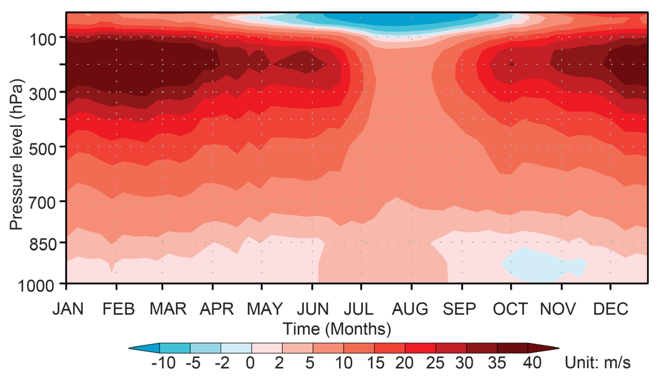
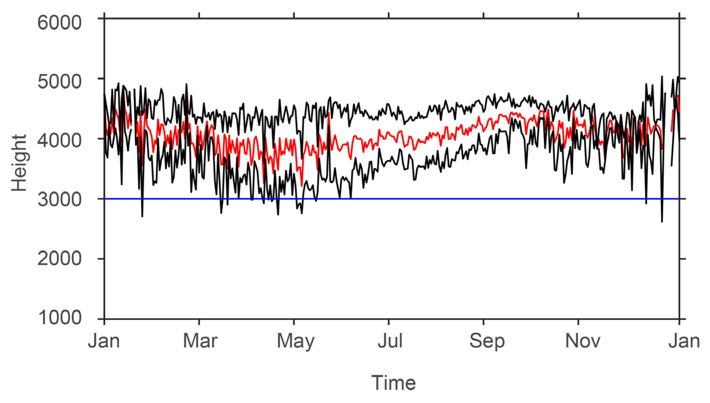
The meteorological factors around the Tibetan Plateau satisfy conditions in which a stable vortex street on the lee side of an obstacle can exist for the whole year. The Froude number varies from 0.2 to 0.3 and falls in the range of Froude numbers that could support vortex shedding for the whole year, whereas the Reynolds number was estimated to be 0.7 × 10⁴–2.4 × 10⁴ in winter and 0.4 × 10⁴–1.2 × 10⁴ in summer. Both of these dimensionless indices fall in the range of meteorological conditions summarized by previous studies [27].
(2)
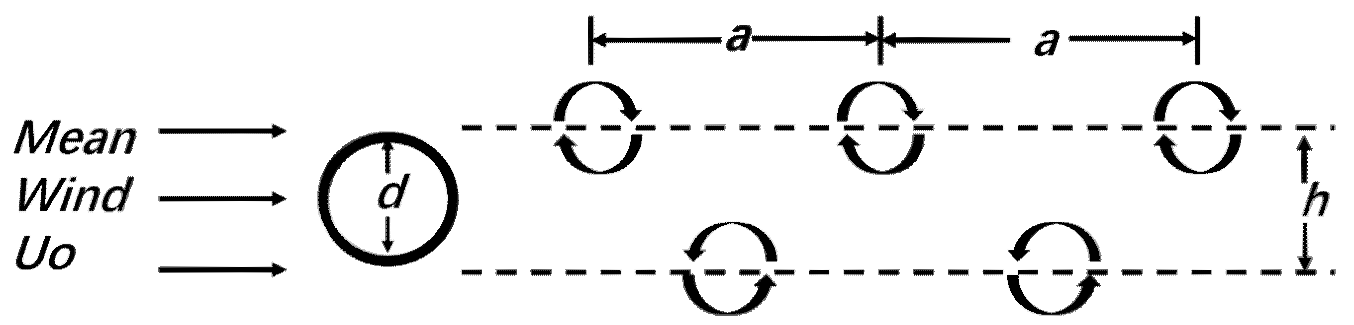
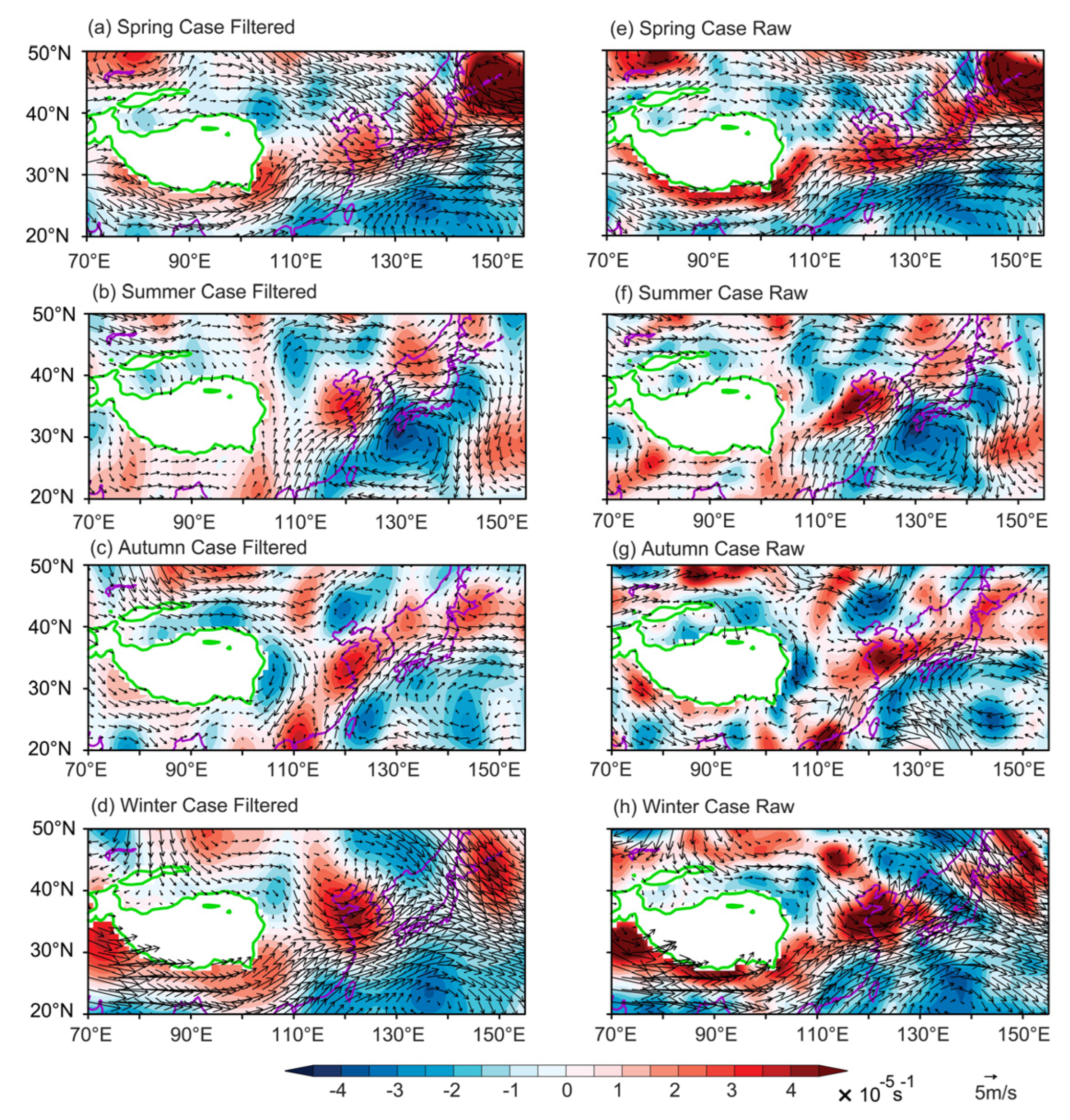
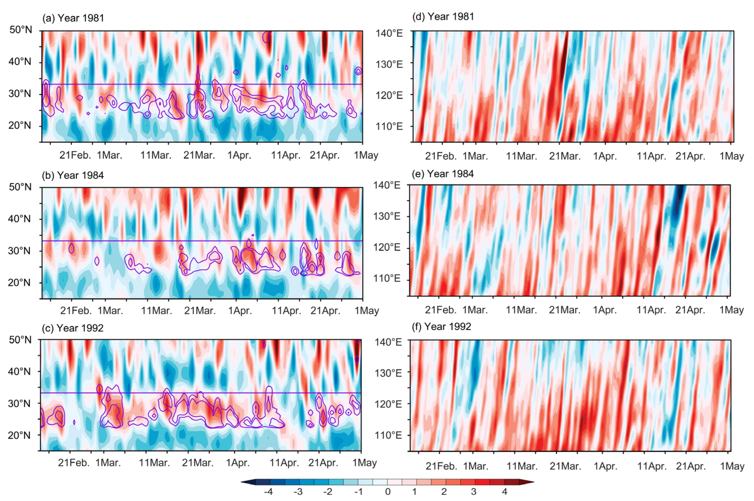
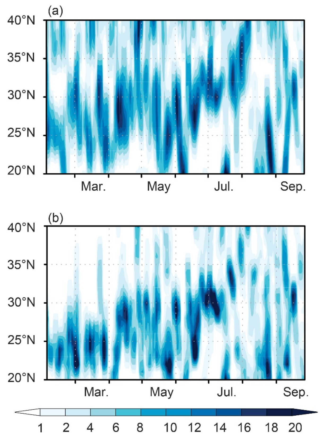
The spatiotemporal structures indicate that the wake on the leeward side of the Tibetan Plateau showed seasonal variations. The wake was characterized by a stable vortex street with a southwest-northeast orientation in summer and early autumn but with a west-east orientation in other seasons. The differences in the centerline orientation among various seasons may be related to the difference in the position of the Western Pacific Subtropical Anticyclone. The wake in the Tibetan Plateau bears a close resemblance to that of the classic von Kármán vortex-street patterns observed in laboratory flow experiments. Moreover, various properties, including aspect ratio, Strouhal number, etc., calculated for these AVSs are in the same range as previous studies. Thus, the wake on the leeward side of the Tibetan Plateau can be interpreted as the atmospheric analog of classic von Kármán vortex streets in various seasons.
(3)
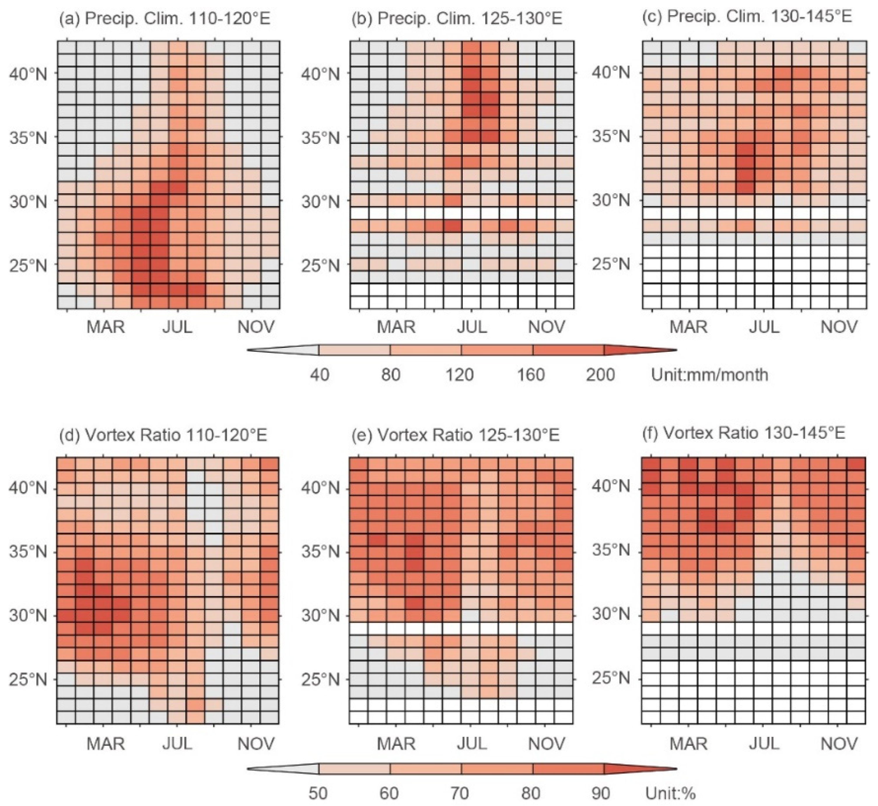
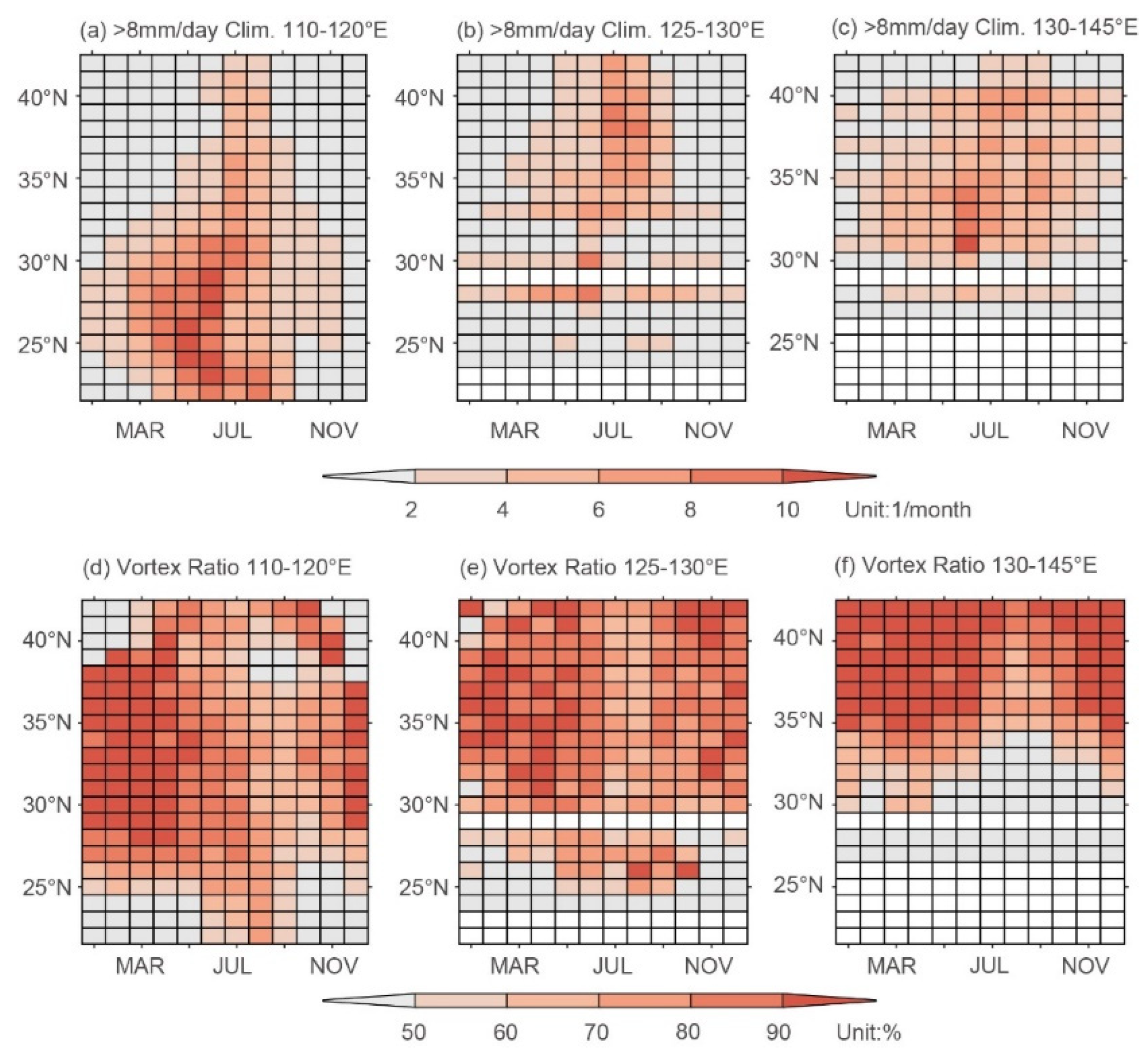
We further show that the spatiotemporal structure of precipitation was largely shared by that of cyclonic activities in the AVS, both in the climatological mean and case study. Approximately 80–90% of the precipitation and heavy rain days in the main rainband over the wake of the Tibetan Plateau are closely tied to the seasonal evolution of the AVS.
Previous studies have suggested that the subtropical convergence zone (the Meiyu-Baiu-Changma frontal zone) is a key circulation system dominating summer precipitation over the wake of the Tibetan Plateau. In this study, the AVS in the subtropics was found on the leeward side of the Tibetan Plateau, spatiotemporally coinciding well with the subtropical convergence zone. Thus, the AVS can be regarded as the dominating mechanism of the subtropical convergence zone. Exploring the underlying relationship between the large-scale circulation and the AVS would help to improve the simulating skill of precipitation over East Asia in numerical simulations in the future.

Author Contributions

Conceptualization, Q.L., Z.W. and C.F.; methodology, Q.L.; validation, Z.W. and F.Y.; formal analysis, Q.L.; investigation, Q.L. and Z.W.; data curation, Q.L.; writing—original draft preparation, Q.L.; writing—review and editing, Z.W., C.F., Z.-M.T. and F.Y.; visualization, Q.L. and Z.W.; supervision, Z.W., C.F. and Z.-M.T.; project administration, Z.W. and C.F.; funding acquisition, C.F. All authors have read and agreed to the published version of the manuscript.

Funding

This research was funded by the Chinese Jiangsu Collaborative Innovation Center for Climate Change, the Frontiers Science Center for Critical Earth Material Cycling of Nanjing University, and the High-Performance Computing Centers of Nanjing University.

Institutional Review Board Statement

Not applicable.

Informed Consent Statement

Not applicable.

Data Availability Statement

The ERA-Interim dataset can be downloaded from the website https://apps.ecmwf.int/datasets/data/interim-full-daily/levtype=sfc/ (accessed on 1 January 2022). The NCEP/NCAR dataset can be downloaded from https://psl.noaa.gov/data/gridded/data.ncep.reanalysis.html (accessed on 1 January 2022). The CPC precipitation data can be downloaded from the website https://psl.noaa.gov/data/gridded/data.cpc.globalprecip.html (accessed on 1 January 2022). The APHRODITE precipitation data can be downloaded from the website http://aphrodite.st.hirosaki-u.ac.jp/products.html (accessed on 1 January 2022).

Conflicts of Interest

The authors declare no conflict of interest.

References

  1. von Kármán, T. Über den Mechanismus des Widerstandes, den ein bewegter Körper in einer Flüssigkeit erfärt. 1. Teil, Nachr. Ges. Wiss. Göttingen. Math.-Phys. Kl. 1911, 1911, 509–517. [Google Scholar]
  2. von Kármán, T. Über den Mechanismus des Widerstandes, den ein bewegter Körper in einer Flüssigkeit erfärt. 2. Teil, Nachr. Ges. Wiss. Göttingen. Math.-Phys. Kl. 1912, 1912, 547–556. [Google Scholar]
  3. Kundu, P.K. Fluid Dynamics; Academic Press: San Diego, CA, USA, 1990; pp. 321–338. [Google Scholar]
  4. Nunalee, C.G.; Basu, S. On the periodicity of atmospheric von Kármán vortex streets. Environ. Fluid Mech. 2014, 14, 1335–1355. [Google Scholar] [CrossRef]
  5. Barton, E.D.; Basterretxea, G.; Flament, P.; Mitchelson-Jacob, E.G.; Jones, B.; Arîstegui, J.; Herrera, F. Lee region of gran canaria. J. Geophys. Res.-Oceans 2000, 105, 17173–17193. [Google Scholar] [CrossRef] [Green Version]
  6. Li, X.; Clemente-Colón, P.; Pichel, W.G. Atmospheric vortex streets on a RADARSAT SAR image. Geophys. Res. Lett. 2000, 27, 1655–1658. [Google Scholar] [CrossRef]
  7. Young, G.S.; Zawislak, J. An observational study of vortex spacing in island wake vortex streets. Mon. Weather Rev. 2006, 134, 2285–2294. [Google Scholar] [CrossRef]
  8. Dong, C.; McWilliams, J.C.; Shchepetkin, A.F. Island wakes in deep water. J. Phys. Oceanogr. 2007, 37, 962–981. [Google Scholar] [CrossRef]
  9. Zheng, Q.; Lin, H.; Meng, J.; Hu, X.; Song, Y.T.; Zhang, Y.; Li, C. Sub-mesoscale ocean vortex trains in the Luzon Strait. J. Geophys. Res.-Oceans 2008, 113, C04032. [Google Scholar] [CrossRef] [Green Version]
  10. Teinturier, S.; Stegner, A.; Didelle, H.; Viboud, S. Small-scale instabilities of an island wake flow in a rotating shallow-water layer. Dyn. Atmos. Oceans 2010, 49, 1–24. [Google Scholar] [CrossRef] [Green Version]
  11. Topouzelis, K.; Kitsiou, D. Detection and classification of mesoscale atmospheric phenomena above sea in SAR imagery. Remote Sens. Environ. 2015, 160, 263–272. [Google Scholar] [CrossRef]
  12. Caldeira, R.M.A.; Groom, S.; Miller, P.; Pilgrim, D.; Nezlin, N.P. Sea-surface signatures of the island mass effect phenomena around Madeira Island, Northeast Atlantic. Remote Sens. Environ. 2002, 80, 336–360. [Google Scholar] [CrossRef]
  13. Caldeira, R.M.A.; Marchesiello, P.; Nezlin, N.P.; DiGiacomo, P.M.; McWilliams, J.C. Island wakes in theSouthern California Bight. J. Geophys. Res.-Oceans 2005, 110, C11012. [Google Scholar] [CrossRef]
  14. Hasegawa, D.; Yamazaki, H.; Lueck, R.G.; Seuront, L. How islands stir and fertilize the upper ocean. Geophys. Res. Lett. 2004, 31, L16303. [Google Scholar] [CrossRef] [Green Version]
  15. Hasegawa, D.; Lewis, M.R.; Gangopadhyay, A. How islands cause phytoplankton to bloom in their wakes. Geophys. Res. Lett. 2009, 36, L20605. [Google Scholar] [CrossRef]
  16. Horváth, Á.; Bresky, W.; Daniels, J.; Vogelzang, J.; Stoffelen, A.; Carr, J.L.; Wu, D.L.; Seethala, C.; Günther, T.; Buehler, S.A. Evolution of an Atmospheric Kármán Vortex Street from High-Resolution Satellite Winds: Guadalupe Island Case Study. J. Geophys. Res.-Atmos. 2020, 125, e2019JD032121. [Google Scholar] [CrossRef] [Green Version]
  17. Lettau, H. Atmosphärische Turbulenz. Akad. Verl. Leipz. 1939, 283. [Google Scholar]
  18. Hubert, L.F.; Krueger, A.F. Satellite Pictures of Mesoscale Eddies. Mon. Weather Rev. 1962, 90, 457–463. [Google Scholar] [CrossRef]
  19. Chopra, K.P.; Hubert, L.F. Kármán vortex streets in earth’s atmosphere. Nature 1964, 203, 1341–1343. [Google Scholar] [CrossRef]
  20. Chopra, K.P.; Hubert, L.F. Mesoscale Eddies in Wake of Islands. J. Atmos. Sci. 1965, 22, 652–657. [Google Scholar] [CrossRef]
  21. Lyons, W.A.; Fujita, T. Mesoscale motions in oceanic stratus as revealed by satellite data. Mon. Weather Rev. 1968, 96, 304–314. [Google Scholar] [CrossRef]
  22. Tsuchiya, K. The clouds with the shape of Kármán vortex street in the wake of Cheju Island, Korea. J. Meteorol. Soc. JPN Ser. II 1969, 47, 457–465. [Google Scholar] [CrossRef] [Green Version]
  23. Zimmerman, L.I. Atmospheric wake phenomena near the Canary Islands. J. Appl. Meteorol. Clim. 1969, 8, 896–907. [Google Scholar] [CrossRef]
  24. Chopra, K.P. Atmospheric and Oceanic Flow Problems Introduced by Islands. In Advances in Geophysics; Academic Press: New York, NY, USA, 1973. [Google Scholar]
  25. Thomson, R.E.; Gower, J.; Bowker, N.W. Vortex Streets in the Wake of the Aleutian Islands. Mon. Weather Rev. 1977, 105, 873–884. [Google Scholar] [CrossRef]
  26. Jensen, N.O.; Agee, E.M. Vortex cloud street during AMTEX 75. Tellus 1978, 30, 517–523. [Google Scholar] [CrossRef]
  27. Etling, D. On atmospheric vortex streets in the wake of large islands. Meteorol. Atmos. Phys. 1989, 41, 157–164. [Google Scholar] [CrossRef]
  28. Li, X.; Zheng, W.; Zou, C.Z.; Pichel, W.G. A SAR Observation and Numerical Study on Ocean Surface Imprints of Atmospheric Vortex Streets. Sensors 2008, 8, 3321–3334. [Google Scholar] [CrossRef] [PubMed] [Green Version]
  29. Couvelard, X.; Caldeira, R.M.A.; Araújo, I.B.; Tomé, R. Wind mediated vorticity-generation and eddy-confinement, leeward of the Madeira Island: 2008 numerical case study. Dynam. Atmos. Oceans 2012, 58, 128–149. [Google Scholar] [CrossRef]
  30. Caldeira, R.M.; Tomé, R. Wake response to an ocean-feedback mechanism: Madeira Island case study. Bound.-Lay. Meteorol. 2013, 148, 419–436. [Google Scholar] [CrossRef] [Green Version]
  31. Ito, J.; Niino, H. Atmospheric Kármán Vortex Shedding from Jeju Island, East China Sea: A Numerical Study. Mon. Weather Rev. 2015, 144, 139–148. [Google Scholar] [CrossRef]
  32. Papailiou, D.D.; Lykoudis, P.S. Turbulent vortex streets and the entrainment mechanism of the turbulent wake. J. Fluid Mech. 1974, 62, 11–31. [Google Scholar] [CrossRef]
  33. Yeh, T. The circulation of the high troposphere over China in the winter of 1945–46. Tellus 1950, 2, 173–183. [Google Scholar] [CrossRef] [Green Version]
  34. Bolin, B. On the Influence of the Earth’s Orography on the General Character of the Westerlies. Tellus 2016, 2, 184–195. [Google Scholar] [CrossRef]
  35. Queney, P. The problem of air flow over mountains: A summary of theoretical studies. Bull. Am. Meteorol. Soc. 1948, 29, 16–26. [Google Scholar] [CrossRef]
  36. Charney, J.G.; Eliassen, A. A numerical method for predicting the perturbations of the middle latitude westerlies. Tellus 1949, 1, 38–54. [Google Scholar] [CrossRef] [Green Version]
  37. Wu, G.X. The nonlinear response of the atmosphere to large-scale mechanical and thermal forcing. J. Atmos. Sci. 1984, 41, 2456–2476. [Google Scholar] [CrossRef]
  38. Wang, Q.; Tan, Z.-M. Multi-scale topographic control of southwest vortex formation in Tibetan Plateau region in an idealized simulation. J. Geophys. Res.-Atmos. 2014, 119, 11543–11561. [Google Scholar] [CrossRef]
  39. Zhang, G.; Mao, J.; Liu, Y.; Wu, G. PV perspective of impacts on downstream extreme rainfall event of a Tibetan Plateau vortex collaborating with a southwest China vortex. Adv. Atmos. Sci. 2021, 38, 1835–1851. [Google Scholar] [CrossRef]
  40. Wu, G.; Tang, Y.; He, B.; Liu, Y.; Mao, J.; Ma, T.; Ma, T. Potential vorticity perspective of the genesis of a Tibetan Plateau vortex in June 2016. Clim. Dyn. 2022, 58, 3351–3367. [Google Scholar] [CrossRef]
  41. Zhang, J.; Li, J.; Guo, B.; Ma, Z.; Li, X.; Ye, X.; Yu, H.; Liu, Y.; Yang, C.; Zhang, S.; et al. Magnetostratigraphic age and monsoonal evolution recorded by the thickest Quaternary loess deposit of the Lanzhou region, western Chinese Loess Plateau. Quat. Sci. Rev. 2016, 139, 17–29. [Google Scholar] [CrossRef]
  42. Dee, D.P.; Uppalaa, S.M.; Simmonsa, A.J.; Berrisforda, P.; Polia, P.; Kobayashib, S.; Andraec, U.; Balmasedaa, M.A.; Balsamoa, G.; Bauera, P.; et al. The ERA-Interim reanalysis: Configuration and performance of the data assimilation system. Q. J. R. Meteorol. Soc. 2011, 137, 553–597. [Google Scholar] [CrossRef]
  43. Kalnay, E.; Kanamitsu, M.; Kistler, R.; Collins, W.; Deaven, D.; Gandin, L.; Iredell, M.; Saha, S.; White, G.; Woollen, J.; et al. The NCEP/NCAR 40-Year Reanalysis Project. Bull. Am. Meteorol. Soc. 1996, 77, 437–471. [Google Scholar] [CrossRef]
  44. Curio, J.; Schiemann, R.; Hodges, K.I.; Turner, A.G. Climatology of Tibetan Plateau vortices in reanalysis data and a high-resolu- tion global climate model. J. Clim. 2019, 32, 1933–1950. [Google Scholar] [CrossRef]
  45. Chen, M.; Shi, W.; Xie, P.; Silva, V.B.S.; Kousky, V.E.; Wayne Higgins, R.; Janowiak, J.E. Assessing objective techniques for gauge-based analyses of global daily precipitation. J. Geophys. Res.-Atmos. 2008, 113, D04110. [Google Scholar] [CrossRef]
  46. Yatagai, A.; Arakawa, O.; Kamiguchi, K.; Kawamoto, H.; Nodzu, M.I.; Hamada, A. A 44-Year Daily Gridded Precipitation Dataset for Asia Based on a Dense Network of Rain Gauges. Sola 2009, 5, 137–140. [Google Scholar] [CrossRef] [Green Version]
  47. Wheeler, M.; Kiladis, G.N. Convectively coupled equatorial waves:analysis of clouds and temperature in the wavenumber-frequency domain. J. Atmos. Sci. 1999, 56, 374–399. [Google Scholar] [CrossRef]
  48. Kiladis, G.N.; Wheeler, M.C.; Haertel, P.T.; Straub, K.H.; Roundy, P.E. Convectively coupled equatorial waves. Rev. Geophys. 2009, 47, 2008RG000266. [Google Scholar] [CrossRef]
  49. Hawcroft, M.K.; Shaffrey, L.C.; Hodges, K.I.; Dacre, H.F. How much Northern Hemisphere precipitation is associated with extratropical cyclones? Geophys. Res. Lett. 2012, 39, L24809. [Google Scholar] [CrossRef] [Green Version]
  50. Hanley, J.; Caballero, R. Objective identification and tracking of multicentre cyclones in the ERA-Interim reanalysis dataset. Q. J. R. Meteorol. Soc. 2012, 138, 612–625. [Google Scholar] [CrossRef]
  51. Snyder, W.H.; Thomson, R.S.; Eskridge, R.E.; Lawson, R.E.; Castro, I.P.; Lee, S.T.; Hunt, J.C.R.; Ogawa, J. The structure of strongly stratified flows over hills: Dividing streamline concept. J. Fluid Mech. 1985, 152, 249–288. [Google Scholar] [CrossRef]
  52. Trenberth, K.E.; Chen, S.C. Planetary waves kinematically forced by Himalayan orography. J. Atmos. Sci. 2010, 45, 2934–2948. [Google Scholar] [CrossRef]
  53. Roshko, A. On the Development of Turbulent Wakes from Vortex Streets (No. NACA-TR-1191). Ph.D. Thesis, California Institute of Technology, Pasadena, CA, USA, 1954. [Google Scholar]
Figure 1. Schematic plot of a Kármán vortex street generated by wind passing a cylindrical obstacle of diameter d. a is the vortex spacing and h is the width of the Kármán vortex street.
Atmosphere 14 01096 g001
Figure 2. Vertical-temporal distributions of climatological mean values of the zonal wind at the grid (40° E, 32° N) during 1979–2018 (unit: m/s).
Atmosphere 14 01096 g002
Figure 3. Red line: The seasonal variation in the climatological mean of the height of the dividing streamline hc of the Tibetan Plateau (unit: m). Black lines mark 1 standard deviation. The blue line is the threshold above which the stable AVS could exist.
Atmosphere 14 01096 g003
Figure 4. (ad) Fourier filtered horizontal structure of 4 cases in daily relative vorticity at 700 hPa for the period of boreal (a) spring (16 March 1992), (b) summer (1 August 1991), (c) autumn (15 September 2002), and (d) winter (15 February 2005) (unit: s−1). The green line marks the topography of the Tibetan Plateau. The vector exhibited the Fourier filtered 700 hPa horizontal wind field. (eh) Same as (ad) but for the unfiltered field replacing the Fourier filtered field.
Atmosphere 14 01096 g004
Figure 5. (ac) Hovmöller diagram of daily relative vorticity at 700 hPa averaged over 110–120° E (unit: 10−5 s−1) for the period of February to April (winter to spring) in (a) 1981, (b) 1984, and (c) 1992. The straight line in panel a is used to represent 32° N, which is roughly the central line of the Tibetan Plateau. Precipitation averaged over 110–120° E was also exhibited by the purple lines (2 levels of 5 mm/day and 15 mm/day). (df) Hovmöller diagram of daily relative vorticity at 700 hPa averaged over 28–32° N from March to April in (a) 1981, (b) 1984, and (c) 1992 (unit: 10−5 s−1).
Atmosphere 14 01096 g005
Figure 6. Hovmöller diagram of (ac) daily precipitation derived from CPC datasets (unit: mm) and (df) daily relative vorticity at 850 hPa (unit: 10−6 s−1) averaged over (a,d) 110–120° E, (b,e) 125–130° E, and (c,f) 130–145° E. The results were smoothed by a pentad temporal domain. Gray represents missing records.
Atmosphere 14 01096 g006
Figure 7. Hovmöller diagram of (a) daily relative vorticity at 850 hPa (unit: 10−6 s−1) and (b) daily precipitation derived from CPC datasets (unit: mm) for the period from February to September 1983 averaged over 110–120° E. The results were smoothed by a pentad temporal domain.
Atmosphere 14 01096 g007
Figure 8. Hovmöller diagram of the (ac) monthly precipitation and (df) the ratio of the monthly precipitation closely tied to AVS to the total monthly precipitation averaged over (a,d) 110–120° E, (b,e) 125–130° E, and (c,f) 130–145° E. White represents missing records of land precipitation.
Atmosphere 14 01096 g008
Figure 9. Hovmöller diagram of (ac) the yearly frequency of heavy rain days (defined as daily precipitation exceeding 8 mm/day) and the ratio of (df) the number of heavy rain days closely tied to AVS to the total number of heavy rain days averaged over (a,d) 110–120° E, (b,e) 125–130° E, and (c,f) 130–145° E. White represents missing records of land precipitation.
Atmosphere 14 01096 g009
Table 1. Characteristic values for the vortex streets of the leeward side of the Tibetan Plateau for 12 cases in spring and winter. The characteristic values include vortex spacing a, vortex width h, and aspect ratio h/a, AVS vortex shedding period Te, the propagation velocity of the AVS patterns Ue, the undisturbed wind velocity Uo, the Reynolds number Re, and the Strouhal number S.
Datea (km)h (km)h/aUe (m/s)Uo (m/s)Te (hour)ReS
1981/3/18279111960.462 5.66 7.281377.28 × 1030.279
1981/4/830745250.201 10.40 19.40821.24 × 1040.273
1981/4/19247814580.588 8.39 9.99821.56 × 1040.216
1981/4/2434407410.217 11.12 20.74861.59 × 1040.204
1984/3/14308710830.381 7.20 10.271198.58 × 1030.272
1984/4/7319510880.343 17.78 28.38502.27 × 1040.245
1984/4/2126229820.366 9.11 13.27801.70 × 1040.205
1984/4/2530369890.326 10.27 17.29821.22 × 1040.278
1992/3/23353810230.327 13.83 23.28711.97 × 1040.198
1992/2/15380712980.24112.9524.14862.41 × 1040.133
1992/4/1357610660.313 9.20 17.15 1081.71 × 1040.150
2004/2/15298712110.2688.4315.721081.57 × 1040.164
Table 2. Characteristic values for the vortex streets of the leeward side of the Tibetan Plateau for 12 cases in summer. The characteristic values include vortex spacing a, vortex width h, and aspect ratio h/a, AVS vortex shedding period Te, the propagation velocity of the AVS patterns Ue, the undisturbed wind velocity Uo, the Reynolds number Re, and the Strouhal number S.
Datea (km)h (km)h/aUe (m/s)Uo (m/s)Te (hour)ReS
1981/8/1213928250.594 5.95 7.08658.66 × 1030.493
1981/8/1622708420.376 5.84 8.331087.45 × 1030.345
1981/8/2019789110.465 6.96 8.87791.17 × 1040.300
1981/8/24179510700.600 5.60 6.65891.04 × 1040.299
1984/7/2252014720.591 6.09 7.251151.02 × 1040.236
1984/7/618428410.475 3.60 4.561424.63 × 1030.422
1984/7/1017908260.469 3.50 4.461424.82 × 1030.406
1984/7/1420245630.291 5.98 11.14947.25 × 1030.407
1992/7/2220410080.457 4.90 6.301259.13 × 1030.243
1992/7/614838240.552 4.21 5.10984.92 × 1030.576
1992/7/1013838770.635 2.49 2.921543.49 × 1030.517
1992/7/14168712930.767 3.04 3.451543.45 × 1030.523
Disclaimer/Publisher’s Note: The statements, opinions and data contained in all publications are solely those of the individual author(s) and contributor(s) and not of MDPI and/or the editor(s). MDPI and/or the editor(s) disclaim responsibility for any injury to people or property resulting from any ideas, methods, instructions or products referred to in the content.

