Article

Investigating the Effect of Fuel Moisture and Atmospheric Instability on PyroCb Occurrence over Southeast Australia

1
School of Science, University of New South Wales, Canberra, ACT 2612, Australia
2
ARC Centre of Excellence for Climate Extremes, UNSW Canberra, Canberra, ACT 2610, Australia
*
Author to whom correspondence should be addressed.
Atmosphere 2023, 14(7), 1087; https://doi.org/10.3390/atmos14071087
Submission received: 23 April 2023 / Revised: 26 June 2023 / Accepted: 27 June 2023 / Published: 28 June 2023

Abstract

:
The incidence of pyro-cumulonimbus (pyroCb) caused by extreme wildfires has increased markedly in Australia over the last several decades. This increase can be associated with a dangerous escalation of wildfire risk and severe stratospheric pollution events. Atmospheric and fuel conditions are important influences on pyroCb occurrence, but the exact causal relationships are still not well understood. We used the Continuous Haines Index (C-Haines) to represent atmospheric instability and the Fuel Moisture Index (FMI) to represent fuel moisture to provide better insight into the effects of atmospheric and fuel conditions on pyroCb occurrence over southeast Australia. C-Haines and FMI were related to the probability of pyroCb occurrence by employing a logistic regression on data gathered between 1980 and 2020. Emphasis is placed on investigating the independent effects and combined effects of FMI and C-Haines, as well as assessing their potential to predict whether a pyroCb develops over a fire. The main findings of this study are: (1) high C-Haines and low FMI values are representative of favorable conditions for pyroCb occurrence, but C-Haines can offset the effect of FMI—the addition of C-Haines to the logistic model muted the significance of FMI; (2) among the components of C-Haines, air temperature lapse rate (CA) is a better predictor of pyroCb occurrence than the dryness component (CB); (3) there are important regional differences in the effect of C-Haines and FMI on pyroCb occurrence, as they have better predictive potential in New South Wales than in Victoria.

1. Introduction

Extreme wildfire events associated with violent pyro-convection have recently occurred in Australia and other regions of the world. In some of these events, violent pyro-convection has manifested as pyro-cumulonimbus clouds (pyroCbs), which not only impact the surface but may also extend their influence high into the atmosphere. Depositing aerosols, such as smoke and ash, can be injected into the stratosphere by pyroCbs and then transported around the globe [1,2]. Moreover, pyroCbs sometimes produce lightning [3,4,5], damaging winds, and even spawn tornadoes [6,7], leading to unpredictable fire behavior and dangerous escalation in the risk of a wildfire [8,9]. The incidence of pyroCbs has increased markedly in recent years, particularly in the spring and summer of the 2019–2020 (Black Summer) fire season, when about 33 pyroCbs resulted in aerosol mass consistent with the magnitude of a mid-sized volcanic eruption being injected into the lower stratosphere [10,11,12], resulting in record-breaking levels of observed aerosols in the southern hemisphere [13]. Additionally, the aerosol emissions from this extreme wildfire event led to ozone depletion in the Southern Hemisphere and an increase in the area of the 2020 Antarctic ozone hole [14], as well as triggering phytoplankton blooms in the Southern Ocean [15]. In the past, pyroCbs generally occurred as spatiotemporally isolated events, but during the Black Summer, multiple pyroCbs occurred simultaneously at a regional scale, and climate projections indicate that extreme wildfires will become more frequent and intense in the future [16], suggesting that pyroCb events have the potential to become a more common large-scale hazard. Given the increasing number of pyroCbs and their widespread impact on the environment and socio-economic systems, there is an imperative to understand the conditions under which pyroCbs develop on a regional scale, so that extreme fire management plans can be refined.
PyroCb development is a dynamic process of fire-atmospheric coupling that is driven by the interaction of large and vigorous wildfires and favorable meteorological conditions. Most pyroCb events begin with an extreme fire capable of developing a deep convective plume, while requiring instability and moisture aloft to facilitate condensation, latent heat release, and subsequent enhancement of the buoyancy of growing convective cells [9,17,18,19]. Therefore, analysis and prediction of pyroCb development is often based on atmospheric indices, which measure atmospheric instability, and surface-based fire risk indices, which measure the potential for fire development.
An index commonly used in Australia to monitor atmospheric instability is the Continuous Haines Index (C-Haines) [20]. The original Haines index [21] was designed to indicate the potential for varying degrees of lower tropospheric instability and dryness to influence wildfires under conditions typical of the northwest of the United States. Subsequent studies that investigated the Haines index in different world regions found considerable regional variation in index values [22,23,24]. Specifically, Mills and McCaw [20] found the original Haines index was not configured to identify the most extreme conditions in Australia due to the different temperature-lapse and humidity climatology of the two continents. They consequently extended the Haines index to allow for higher values than the original formulation, rendering it more suitable for Australia where high index values occur frequently. C-Haines provides a measure of the potential for enhanced wildfire behavior. It is based on the temperature lapse rate between the 850 hPa and 700 hPa pressure levels and the dewpoint depression at 850 hPa. High C-Haines values imply drier and more unstable lower atmospheric conditions, which favor the lifting of heated air higher into the atmosphere to maintain strong convection and increases the likelihood of a pyroCb occurrence [20]. Previous studies have confirmed that the majority of pyroCbs coincided with high C-Haines levels in Australia, suggesting C-Haines may provide additional and independent information to that provided by traditional fire danger indices [20,25,26].
A surface-based fire risk index commonly used in Australia is the McArthur Forest Fire Danger Index (FFDI), which considers surface air temperature, relative humidity, wind speed, and precipitation [27]. However, while FFDI is a good indicator of fire risk, it does not perform well as a predictor of a pyroCb occurrence. Previous studies have found that pyroCbs occur over a wide range of FFDI values [28]. However, fuel moisture content has been found to potentially be an indicator of a pyroCb occurrence. Fuel moisture content is directly related to fire behavior—low fuel moisture favors areal flaming, which is strongly associated with extreme fires capable of developing into pyroCbs [8,29]. The Fuel Moisture Index (FMI) [30] is a simple and easily calculated index for assessing fuel moisture that can be used to assess fire danger. FMI has been shown to produce reliable estimates of fuel moisture content in a variety of fine fuel types [30,31,32] and has been validated in field-based studies [33] and been widely used in fire risk assessment [16,34]. A previous study also showed the potential of FMI in assessing pyroCb occurrence—pyroCbs only occurred on days with regional FMI < 6 in NSW (New South Wales) during Australia’s Black Summer [26].
Although C-Haines and FMI have both been confirmed to be associated with pyroCb occurrence to some extent, that extent has not been quantified and their combined effects and potential power to predict pyroCb occurrence is not well understood. Using ERA5 reanalysis, we calculated C-Haines and FMI corresponding to standard wildfires (non-pyroCb-producing) and pyroCb events occurring in the southeast of the Australian mainland from 1980–2020. We then investigated the effects of FMI and C-Haines on pyroCb occurrence using logistic regression models. We conducted three primary investigations: (1) We used univariate and multivariate models to evaluate the independent influence and the combined effect of FMI and C-Haines on pyroCb occurrence; (2) we investigated the respective roles of the temperature lapse and dryness content components of C-Haines; and (3) we assessed the regional differences and the potential power of FMI and C-Haines to predict pyroCb occurrence in fires of different scales. Overall, this study established the relationship between surface fuel moisture content and atmospheric conditions, represented by the FMI and C-Haines, respectively, and pyroCb occurrence at a regional scale using statistical modeling. The aim is to provide insights into the effect and predictive potential of FMI and C-Haines for causing a regular wildfire to develop into a pyroCb. This research improves understanding of the factors influencing pyroCb occurrence at regional scales, thereby contributing to the improvement of regional predictions and management plans for extreme wildfires.

2. Materials and Methods

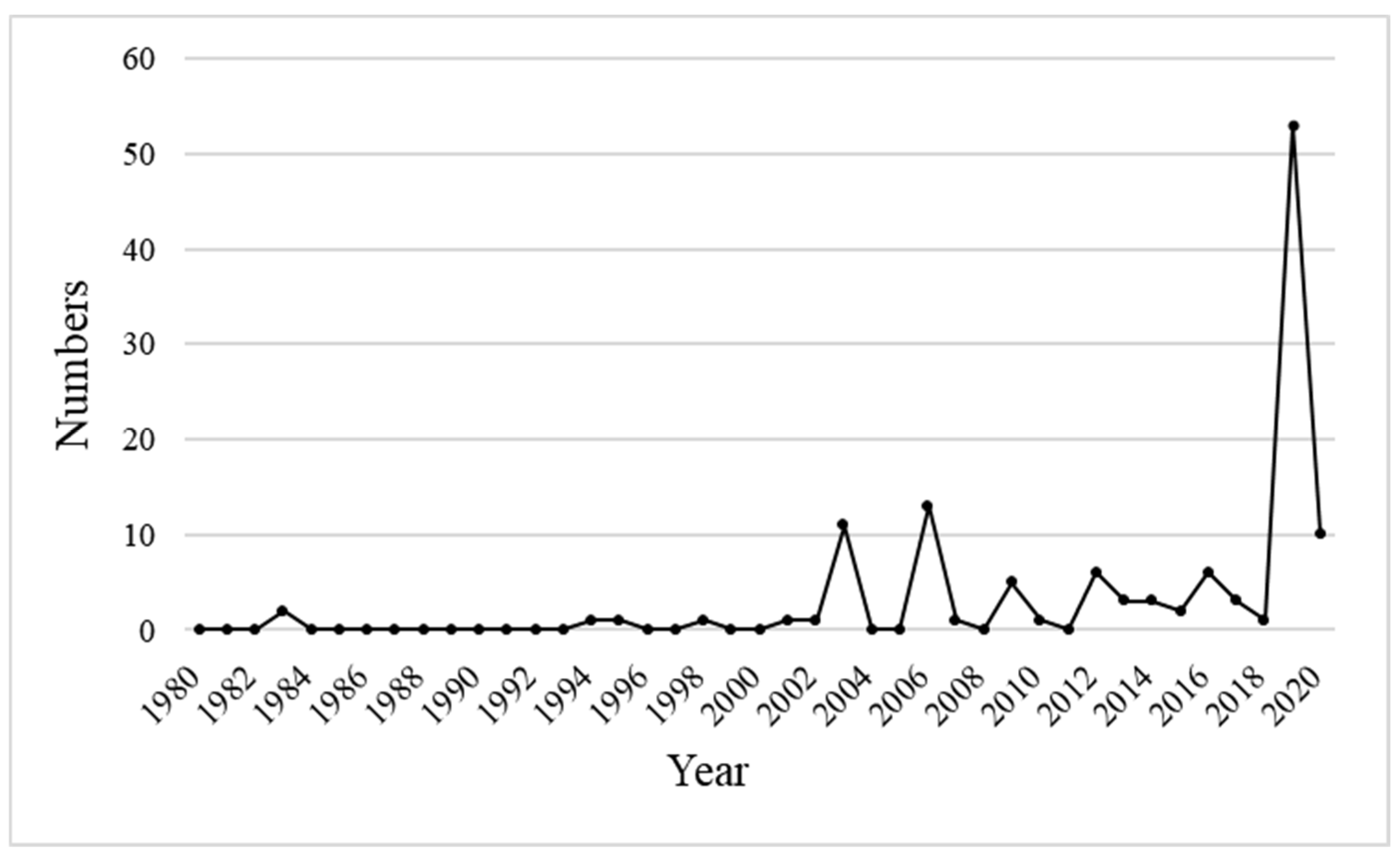
2.1. PyroCb Catalogue
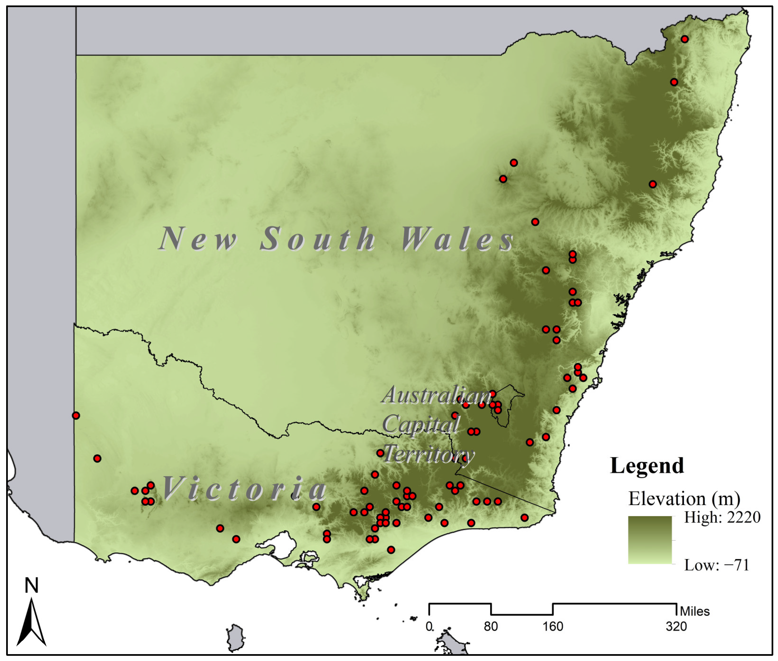
PyroCbs were identified using the Australian PyroCb Register [35] (see Table S1). Table 1 shows the numbers of pyroCbs occurring in each state (Australian Capital Territory, ACT, is included in NSW) in Australia between 1980 and 2020. In terms of their spatial distribution, pyroCbs occur in Vic (42.4%), NSW (32.0%), and WA (22.4%). The highest proportion of pyroCbs occurred in 2019 (42.4%, Figure 1), although pyroCbs have occurred on a reasonably regular basis since about the year 2002. The fuel type in which pyroCbs occurred also has distinctive regional characteristics. We extracted the fuel type of pyroCbs for the states (NSW, Vic, and WA) where pyroCbs occur and found that pyroCbs occurred mostly in forests and woodlands in NSW and Vic but in shrublands and grasslands in WA (Table 2). The fuel type data was sourced from the National Vegetation Information System (NVIS) [36]

2.2. Study Area

Most pyroCbs in Australia occurred in NSW, Victoria and Western Australia, but due to the geographical location and fuel type of pyroCbs in WA being quite different from NSW and Vic, this study only focuses on the southeast of Australia, including the mainland of NSW (including ACT) and Vic (Figure 2). The dominant land-cover types in this region are open shrublands (39%), croplands (26%), evergreen broadleaf forests (13%) and woody savannas (10%) [37]. The climate in this region is temperate: cold and damp in winter, hot and dry in summer.

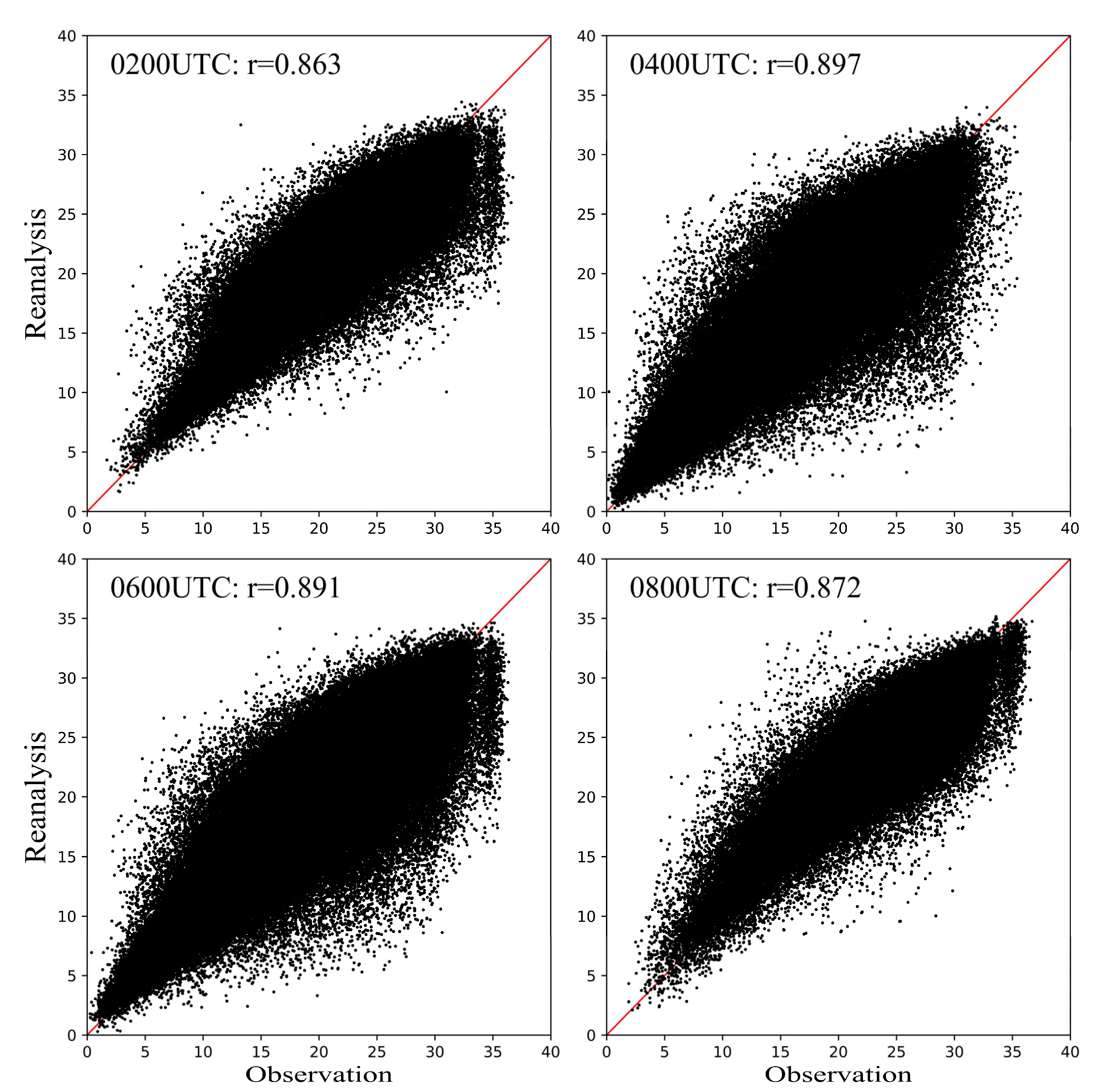
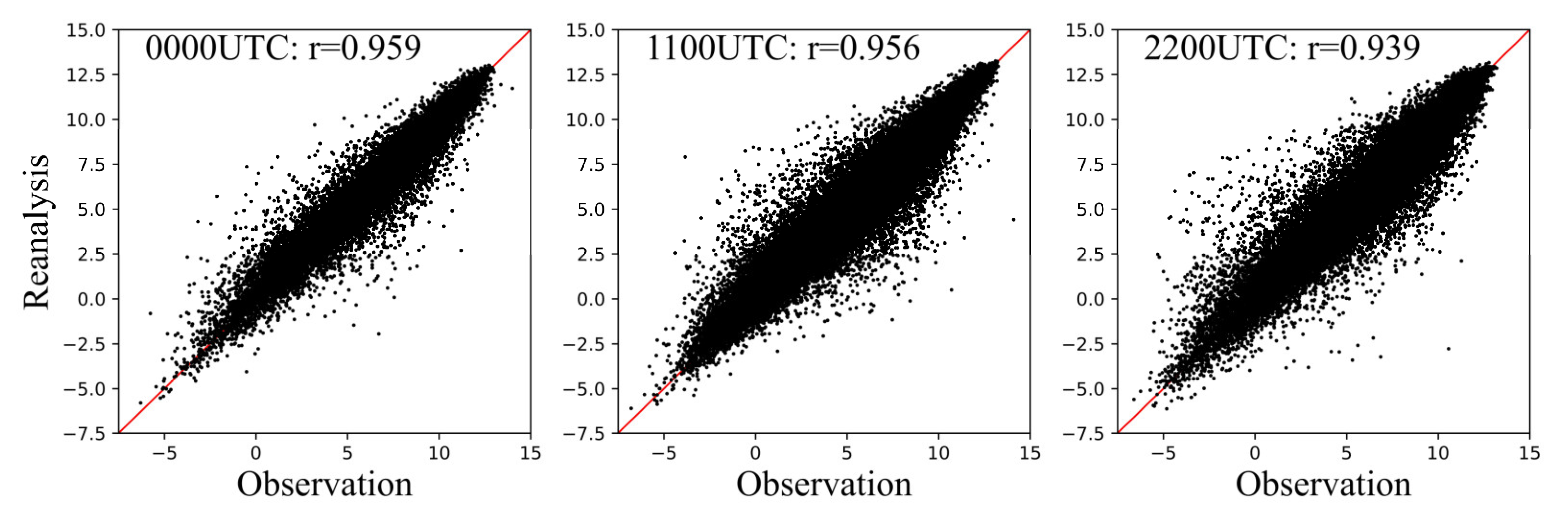
2.3. Data Description

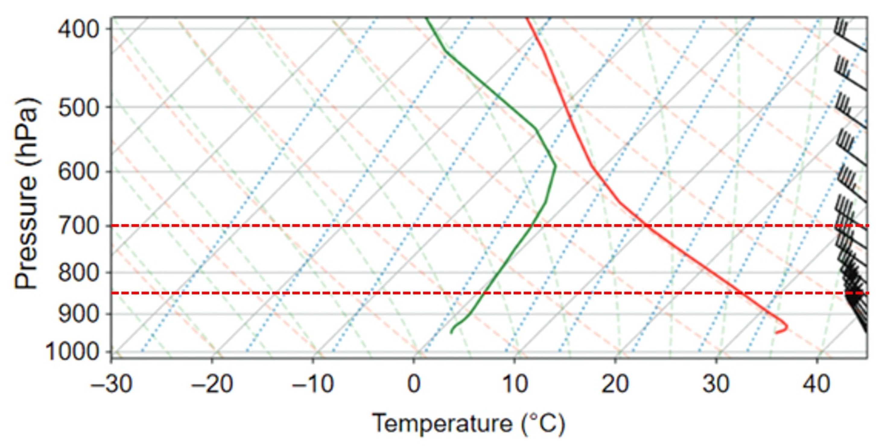
2.3.1. Dependent Variables

The dependent variables in this study have two categories—pyroCbs and standard wildfires (non-pyroCb-producing). The source of the pyroCb data—the Australian PyroCb Register—is an evolving dataset [35]. This register is the result of a collaborative global effort, involving close engagement with Members of the Worldwide PyroCb Information Exchange [38]. It is generated by analyzing remote observation information to assess whether it meets the threshold for a pyroCb [2]. Principal remote data sources include LANDSAT imagery to confirm the burn scars characteristic of pyroCbs; MODIS hot spots to detect large patches without hotspots indicative of rapid burnout of fuels consistent with a blow-up event; and radar data to confirm the event date [7,28]. The Register records the date and location of pyroCbs, but most pyroCbs in the Register did not have the exact time of occurrence, except for the 40 pyroCbs occurring after 2019. In this study, 40 pyroCb events were recorded as occurring in NSW and 53 events recorded as occurring in Victoria from 1980–2020.
Standard wildfires were defined as wildfires that did not produce pyroCbs and were a subset of the government fire history databases in NSW [39] and Victoria [40]. When investigating the fire history datasets, several issues were identified that had to be rectified before the databases could be used in this study. The first issue was related to the start and end dates of fires. Since the government fire history databases were produced by different departments and States, the attributes are inconsistent, e.g., NSW records both the start and end dates of fires, while Victoria records only the start date. Moreover, each state has several fires without any date. Additionally, in the Victoria dataset, 1 January has at times been used to as a default to represent an unknown fire start date. This is of course inconvenient, as 1 January is a date that falls in the heart of Victoria’s annual fire season. The second issue is related to the fire polygons. In more recent years, one wildfire is often represented by multiple polygons, particularly in Victoria. For example, Figure S4 shows two adjacent fires, which surprisingly included 98,103 polygons in the Victoria fire history database.
Due to these issues, a three-step pre-processing of the fire history dataset was performed: (1) Polygons with the same attributes (e.g., date, fire number, fire name) were merged using ESRI ArcMap 10.2 and then were manually checked so that incorrect mergers could be fixed. However, for some polygons with missing attributes, we were unable to identify which fire it belonged to, so we removed these unidentifiable polygons. (2) Fires without any dates were removed. (3) Fires with a date of 01/01/xxxx were manually checked, and, if they did not have a fire number or name and consisted of multiple polygons in widely separated locations, they were regarded as fires with unknown dates and were removed.
We then used the processed fire history data to filter the standard wildfires based on three principles: (1) it was larger than 10 ha; (2) the recorded fire type was “bushfire” (i.e., not a prescribed burn); (3) the fires were not within a 20-km radius of pyroCb locations on pyroCb dates. Due to the fact that the Victorian database did not record the end date of the fire, we did not know how long they lasted and could not determine if any pyroCbs occurred during those fires, so we assumed that they all lasted one month. Therefore, in the process of filtering standard wildfires, for fires with no end date that occurred within 20 km of a pyroCb, we removed those that occurred within one month before the pyroCb date.
Given that the occurrence pattern of pyroCbs varies among regions and fire scales, we divided all pyroCb-producing and standard wildfires into different categories based on location and fire size (Table 3).

2.3.2. Explanatory Variables

For the regression modeling in our study, the explanatory variables are FMI, C-Haines and its two components—the temperature lapse rate between the 850 hPa and 700 hPa pressure levels (CA) and 850 hPa dewpoint depression (CB). C-Haines was used to represent atmospheric instability and FMI was used to represent fuel moisture. These have been commonly used in Australian fire risk assessments and have been shown to be associated with pyroCb development to some extent [20,25,26].
The C-Haines Index is based on tropospheric air temperature lapse rate and dryness content and is used to represent atmospheric instability and dryness. C-Haines is defined as follows [20]:
C A = 0.5 T 850 T 700 2
C B = 0.3333 T 850 D P 850 1
if   T 850 D P 850 > 30 ,   then   T 850 D P 850 = 30
if   C B > 5 ,   then   C B = 5 + C B 5 / 2
C H = C A + C B
where C H is C-Haines index, T 850 and T 700 are the temperatures at the 850 hPa and 700 hPa pressure levels, respectively, and D P 850 is the dewpoint temperature at 850 hPa. C-Haines was calculated using the ERA5 hourly reanalysis on pressure levels [41], with a grid spacing of 0.25° for both latitude and longitude.
The Fuel Moisture Index (FMI) was calculated as [30]:
F M I = 10 0.25 T H
where H is the surface relative humidity and T is the surface dry-bulb temperature. T and H were obtained from the ERA5 hourly reanalysis on single levels [42], in which T is the temperature 2 m above ground level (AGL) and H is calculated from the dewpoint and temperature (2 m AGL) using the MetPy package of python.
Since the exact time of occurrence is unknown for some pyroCbs and no exact time data are available for the occurrence of standard fires, this study focused on mid-afternoon conditions (0600 UTC, 16:00 AEST), as this is when dangerous fire weather conditions most commonly occur in Australia [25]. Additionally, C-Haines and FMI were also calculated for other times in the afternoon (0200 UTC, 0400 UTC and 0800 UTC) to supplement the analysis.
The FMI and C-Haines index values calculated from the ERA5 hourly reanalysis were compared to values calculated using observational data obtained from the Bureau of Meteorology (BoM). The correlation coefficients for FMI values derived from reanalysis and observed data in the afternoon (0200UTC, 0400UTC, 0600UTC and 0800UTC) were high (ranging from 0.863 to 0.897, see Figure 3). C-Haines values derived from reanalysis data were also compared to values calculated using upper-air observations. Fifteen stations have upper-air data from 1980 to 2020 in NSW and Victoria, but the length of record varies at each station. Station records were checked, and it was found that most of the records were at 0000UTC, 1100UTC, and 2200UTC, so C-Haines values at these three times were compared. The C-Haines values calculated from the reanalysis data show strong correlations to those calculated from observational data, with correlation coefficients [43] ranging from 0.94 to 0.96 (Figure 4).

2.4. Modelling Approach

To estimate the probability of a pyroCb occurrence, we developed a logistic regression model. The logistic regression model is a generalized linear model (GLM) [44], which is an extension of linear regression models that is used to estimate the probability of an event using the logit transformation [45]. The logistic regression model can be defined as:
ln P 1 P = β 0 + β 1 x 1 + β 2 x 2 + + β n x n ,
where P is the probability of pyroCb occurrence, x i ,   i = 0 , 1 , , n are explanatory variables, β i ,   i = 0 , 1 , , n , are coefficients that need to be estimated. Under this model ansatz, the probability of pyroCb occurrence can be expressed as:
P y = 1 | x 1 , x 2 x n = 1 1 + e β 0 + β 1 x 1 + β 2 x 2 + + β n x n .
We specified a binary logistic model that has a binary dependent variable coded by 1 and 0 to indicate the occurrence and non-occurrence of a pyroCb.
In this study, the dependent variables are pyroCbs (set as “1”) and “standard wildfires” (set as “0”). The explanatory variables are FMI, C-Haines and the components of C-Haines—CA and CB. We developed both univariate and multivariate models to evaluate the independent influence and the combined influence of FMI and C-Haines on pyroCb occurrence. The univariate model contains only a single explanatory variable, while the multivariate model contains a combination of FMI with C-Haines, CA and CB. We used the p-values to assess whether the given variable had a significant effect on pyroCb occurrence and the coefficients to assess the influence mechanism of the given variables. A positive coefficient indicates that the variable is positively related with the probability of pyroCb occurrence, while a negative coefficient indicates a negative relationship.
To investigate the impact pattern of C-Haines and FMI on pyroCb occurrence in different states and different fire sizes, we initially developed separate models for the 12 subsets in NSW, Victoria and the whole study area, with four different fire sizes. However, the subsets have two problems: (1) the numbers of dependent variables are unbalanced—there are many more standard wildfires than pyroCb-producing fires (an order of magnitude difference in some subsets), which may affect the accuracy of the model results; (2) the ratios of pyroCbs to standard wildfires in these subsets are different, which may cause additional errors in result comparisons (Table 1).
To overcome these problems, a random sampling process was performed for standard wildfires: 50 standard wildfires were randomly selected from each subset of NSW and Victoria, and 100 standard fires (50 from NSW and 50 from Vic) are randomly selected from the whole area to ensure that the ratios of pyroCbs and standard wildfires are close to 1:1 in each model. The random sampling process was repeated 100 times in each subset. Finally, in each subset there were 100 models, and we calculated the mean value of coefficients and p-values for each variable within these 100 models for the final analysis.

3. Results

3.1. The Effect of FMI and C-Haines on pyroCb Occurrence

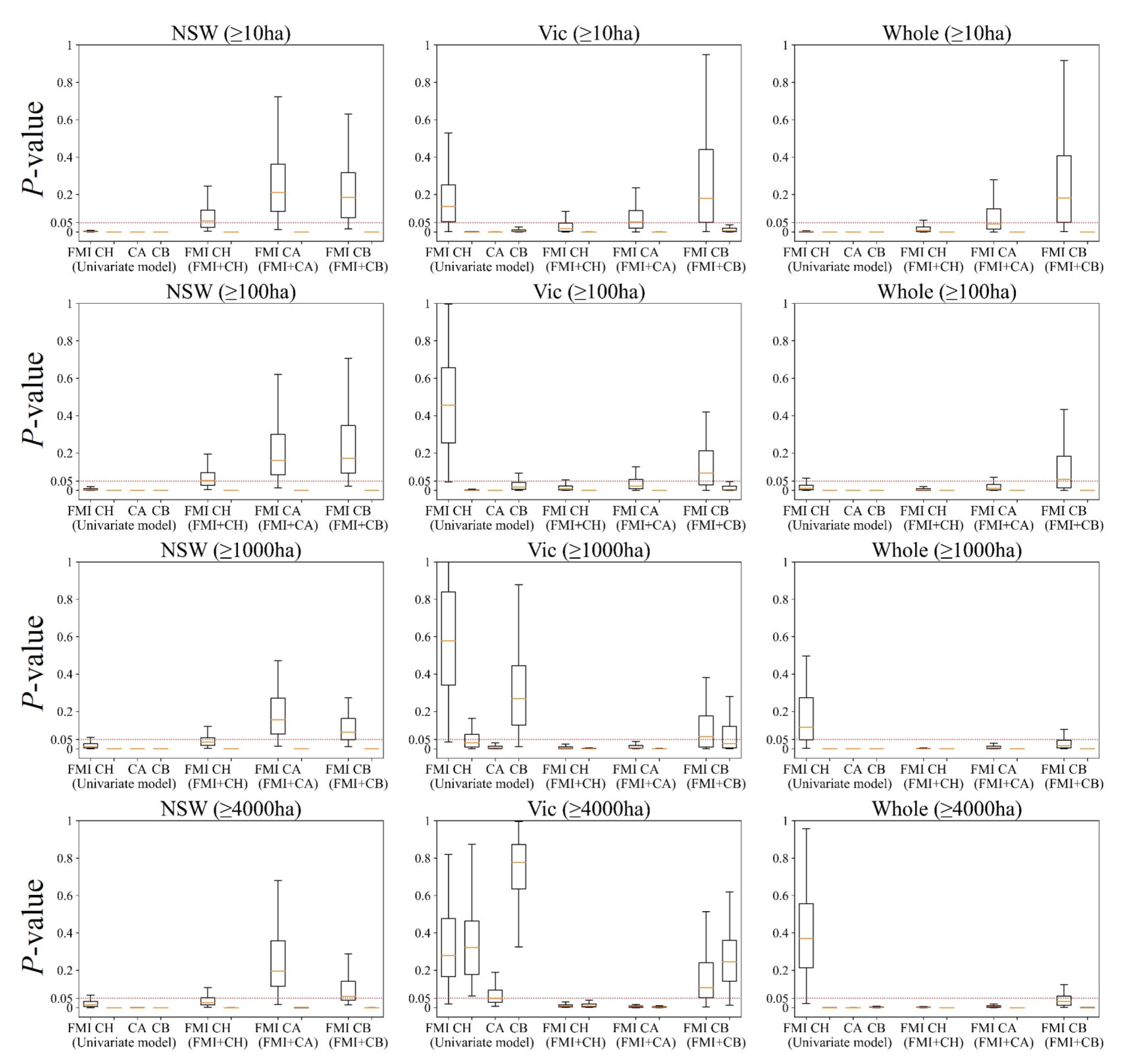
3.1.1. Univariate Models

The first four bars of each subgraph in Figure 5 show the distribution of p-values for each variable in the univariate models at 0600 UTC. In NSW, the mean p-values of all variables in each subset are less than 0.05, indicating that FMI, C-Haines, CA, and CB each have a significant, independent effect on pyroCb occurrence. The situation in Victoria is quite different from that in NSW. In Victoria, the mean p-values of FMI are greater than 0.05 in all subsets. For C-Haines, the mean p-values are less than 0.05 in the subsets with small standard wildfires, but the p-values increase as the standard wildfires become larger and exceed 0.05 in the ≥4000 ha category, suggesting a diminished, or even insignificant, effect of C-Haines on pyroCb development in extremely large fires in Victoria. The mean p-values for CA are significantly smaller than those for C-Haines and CB, suggesting that CA is a better variable for assessing pyroCb development in Victoria. However, in general, univariate models have limited ability and poor effectiveness in assessing pyroCb development in Victoria. For the whole area, C-Haines and its components are highly significant, similar to what was found in NSW, while the p-value of FMI is closer to that of Vic, especially in large wildfires.
Table 4 shows the mean values of the coefficients for each variable. The coefficients of FMI are negative and those of C-Haines, CA and CB are positive in the univariate models where these variables are significant, indicating that FMI is negatively related to the probability of pyroCb occurrence, while C-Haines, CA and CB are positively related.

3.1.2. Multivariate Models

The last six bars of each subgraph in Figure 5 show the distribution of p-values for each variable in the multivariate models at 0600UTC. In NSW, when FMI was combined with C-Haines, the distribution of p-values for FMI was larger than those in the univariate models, even exceeding 0.05 in the two subsets with small standard wildfires (larger than 10 ha and 100 ha), while the p-values for C-Haines are still less than 0.05. CA and CB have similar effects on FMI as well. This suggests that in multivariate models, the effect of FMI may be offset by C-Haines as well as its components, especially in small fires. For larger fires (larger than 1000 ha and 4000 ha), this offset is also present but attenuated.
Interestingly, the situation is different in Victoria, where the combination of FMI and C-Haines has more significant effects than single variables on pyroCb development. FMI is not significant in all univariate models but becomes significant when C-Haines is added to the models. The same is true for C-Haines, which is not significant in the univariate model in the two subsets with larger standard wildfires (larger than 1000 ha and 4000 ha) but becomes significant in the multivariate models. Similar effects are found for CA, but not for CB. Overall, multivariate models are better than univariate models in assessing pyroCb development in Victoria.
For the whole study area, the mean p-values for C-Haines and its components were consistently below 0.05, as they were in NSW. The mean p-values for FMI for subsets with standard wildfires larger than 10 ha were closer to NSW—C-Haines makes p-values for FMI larger but still below 0.05. Meanwhile the results for subsets with standard wildfires larger than 100 ha, 1000 ha and 4000 ha are closer to Victoria—C-Haines makes p-values for FMI smaller.
Notably, the coefficients of FMI are positive in all multivariate models, which is the opposite of the univariate model, further suggesting that C-Haines and its components may influence the effect of FMI or even override it.
The situation at other local afternoon times has also been modeled (0200UTC, 0400UTC and 0800UTC, see Figures S1–S3). The results were broadly similar across time, but did exhibit some differences. For example, at 0800UTC (6pm AEST), while the effect of FMI in NSW was not offset by C-Haines and remained significant in multivariate models, FMI’s effect becomes insignificant in the multivariate models for Victoria, particularly in the subsets with large standard wildfires, which is contrary to the results of 0600UTC.

3.2. Distribution of C-Haines and FMI Values of pyroCbs and Standard Wildfires

Figure 6 shows the corresponding C-Haines and FMI values for pyroCbs and standard wildfires in this study, and Figure 7 shows the distribution of FMI, C-Haines, CA, CB in different states based on kernel density estimates [34]. In general, pyroCbs occurred with high C-Haines and low FMI, with most pyroCbs in NSW occurring within a narrow range of high C-Haines larger than 10 and low FMI less than 15, while in Vic occurring within a wider range of C-Haines larger than five and FMI less than 25. Figure 7 also shows that the distribution curves of FMI, C-Haines, CA and CB for pyroCbs in NSW are more concentrated with steep peaks, while the distribution curves in Vic are flatter. In NSW, the density peaks of FMI and C-Haines are clearly different for pyroCbs and standard wildfires in each subset, while the peaks are close in Vic, especially in larger fires (Figure 6). This may be one reason why the univariate models do not work well in Vic. Among C-Haines and its components, CA has a more concentrated distribution for pyroCbs, followed by C-Haines, and CB has the widest distribution, so CA tends to have smaller p-values than C-Haines and CB, indicating its effect on pyroCb development is more significant than that of C-Haines and CB.

4. Discussion

We have found that pyroCbs are more likely to occur under conditions of high C-Haines and low FMI values, which is consistent with previous studies [26,28]. Both the C-Haines and FMI independently have predictive ability for pyroCb occurrence, albeit with varying effectiveness across different regions. Independently, C-Haines has a significant effect on pyroCb occurrence in NSW, Victoria (except subsets with standard wildfires ≥4000 ha) and the whole study area. Independently, FMI was not significant in Victoria, and its significance decreased with larger standard wildfire size in NSW and in the whole study area. In general, atmospheric instability measured by C-Haines is a better predictor of pyroCb development than fuel moisture content measured by FMI, especially for fires larger than 1000 ha. This may be because the development of both large fires and pyroCbs is associated with deep, areal flaming that requires dry fuel [29]. Therefore, when a fire can expand over a large area, it already indicates that the FMI may be low, in which case atmospheric instability is more likely to determine whether a pyroCb develops or not. The data distributions in Figure 6 and Figure 7 also show that the distribution of FMI values for large fires is closer to that for pyroCbs, especially in Victoria, which also explains the limited predictive power of FMI in Victoria.
The combined effect of C-Haines and FMI was analyzed with the multivariate models, which showed that the effect of FMI is influenced by C-Haines, and this effect has significant regional differences. In NSW, FMI becomes insignificant when C-Haines is included, while the opposite occurs in Victoria. To further investigate the reasons for this, the components of C-Haines were analyzed. Figure 8 shows the correlation between FMI and C-Haines, CA, and CB. Among C-Haines and its components, CB had the highest correlation with FMI, with absolute values of correlation coefficient ranging from 0.697–0.810 in NSW and 0.689–0.720 in Victoria. This may be related to the calculation method of C-Haines and its components. C-Haines uses fixed pressure levels for calculation, which indeed limits its application in varying topography. However, in southeast Australia, the warm summer days usually associated with significant wildfire activity are typically characterized by a deep planetary boundary layer [46]. Within this well-mixed layer, the dewpoint and temperature lapse rates are approximately constant, so that the dewpoint and temperature traces form a triangular pattern in a skew-T log P thermodynamic diagram, such as can be seen in Figure 9. Moreover, this layer often includes the 850 hPa and 700 hPa levels where C-Haines is determined. Therefore, although the components of C-Haines may not provide precise measurements, they can still offer some reflection of the temperature lapse rate and dewpoint depression of the entire vertical depth between the surface and pyroCb condensation level. Given the triangular geometry, the 850 hPa dewpoint depression, which relates to CB, will be approximately proportional to the surface dewpoint depression, which relates to the surface relative humidity used to calculate FMI. As such, FMI will not be independent of C-Haines and its components under such conditions. Thus, in multivariate models, the effect of FMI may be offset by C-Haines and its components, overriding the significance of FMI found in the univariate models. This is in line with the results for NSW, but the results for Victoria are much less straightforward.
In Victoria, FMI was not significant in univariate models but was significant in multivariate models. This may be because Victorian pyroCbs occurred over a wider range of FMI values, and the distribution of FMI for pyroCbs is relatively flat, as it is for standard wildfires (Figure 6). Therefore, in the univariate models, there is no significant relationship between FMI and the probability of pyroCb occurrence. The significance of FMI in the multivariate model is therefore surprising but may be an artifact of the correlation between FMI and C-Haines.
Among C-Haines and its components, CA is the best predictor of pyroCb occurrence—better than both C-Haines and CB. This is especially true in Victoria, where CA is the only variable that is significant in the univariate models for almost all subsets. This may be because CA, the temperature lapse component, has the potential to identify plume-dominated fire behavior, which is necessary for most pyroCb development [9,17]. But not all plume-dominated fires have sufficient potential to cause a pyroCb, and this process is also influenced by fire intensity, fire geometry, upper wind speed and other meteorological and geographical conditions [28,29,47]. Therefore, high CA can be seen as a necessary condition for pyroCb occurrence, but not a sufficient condition. CB could also be a potential indicator, but the significance of CB has regional differences. CB showed a significant effect on pyroCb occurrence in univariate models for NSW and for the whole study area. However, in Victoria, the p-value of CB for the univariate models becomes larger as standard wildfire size increases and becomes insignificant for the subsets of large standard wildfires (≥1000 ha and 4000 ha). Moreover, the distribution of CB values for pyroCbs is very similar to that of large standard wildfires in Victoria, even distributed in a wider range than large fires (Figure 7). The different results relating to CB in NSW and Vic indicate possible regional differences in the occurrence conditions of pyroCbs, but it cannot be ignored that they also may be caused by the issues with data quality. In addition, the way in which CB is calculated, using the difference between temperature and dewpoint, leads to a negative correlation between CB and FMI (Figure 8). We expect pyroCbs to occur at low FMI, which typically corresponds to high CB, and a drier atmospheric environment. However, it has been noted by some authors that pyroCb development requires a moisture source from the mid-troposphere to facilitate condensation and latent heat release [9,12,48]. Although this moisture source is typically found at a higher level (around 500 hPa) than the level 850 hPa at which CB is calculated, it is still uncertain whether this moisture source would not affect or occur at the lower level. This may lead to a contradiction in analyzing the effect of CB on pyroCb occurrence, reminding us that using CB to measure atmospheric moisture in this context has limitations. Other indicators of atmospheric moisture, such as precipitable water, could be considered as an alternative in future studies on pyroCbs. In this context, CA is a better indicator of whether a fire is able to develop into a pyroCb. Moreover, the effect of CA did not show regional differences and was significant in all subsets, suggesting that CA is a more reliable predictor of pyroCb development than CB. In addition, when CB is not significant, C-Haines also loses some significance by its influence, which again highlights the potential limitations of composite indexes such as C-Haines, and suggests that caution should be exercised in their use as a predictor—the effects of their components may offset each other, weakening the effect of composite indexes.
It is worth noting that using only C-Haines and FMI to predict pyroCb development was not effective in Victoria, especially for large fires. In addition to atmospheric conditions, factors such as fuel load and topography may also have a significant influence on pyroCb development [28]. These factors will be considered in future studies to further analyze the drivers of pyroCb development in Australia—especially in Victoria.
The main limitation of this study was data quality. Since the exact times of some pyroCb occurrences were not recorded, this study mainly focused on conditions at 0600UTC (4 pm AEST) [5,28], but also modeled the situation at other local afternoon times (0200UTC, 0400UTC and 0800UTC, see Figures S1–S3). There is some temporal variation in the model results, suggesting that model results can be influenced by the uncertain time, and so obtaining the exact timing of pyroCb occurrence in future studies could provide more accurate results and deeper and more robust insights into the mechanisms of pyroCb development. The website “Worldwide PyroCb Information Exchange” [38] may provide more detailed pyroCb data for our future studies. In addition, because of inconsistent recording of fire end dates, we were only able to extract C-Haines index and FMI input data for the start date of the fires. However, wildfires often last for several days, or even months, and the conditions of the fire start date may not be an accurate representation for the atmospheric and weather conditions of the entire fire lifespan, which likely affects the accuracy of the results of this paper to some extent. Moreover, there are also significant issues with the standard wildfire database, particularly in Victoria, where some fires consisted of many thousands of polygons (Figure S4) which required extensive pre-processing. The removal of the unidentifiable polygons also resulted in some missing data (i.e., fires that occurred during the study period, but had missing attributes). This could potentially be one of the reasons for the unexpected results in Victoria. We must acknowledge that the credibility of the Victoria results could likely be improved with more complete and reliable data. If more accurate fire history data providing information on fire duration and spread processes were available, we could fully account for atmospheric and surface conditions during the entire fire lifespan, which may help to improve the analysis accuracy. Until such information becomes available to support further analyses, the results for Victorian pyroCb occurrence should be treated as tentative and with appropriate skepticism.

5. Conclusions

There are two main findings in this study: (1) high C-Haines and low FMI values are representative of favorable conditions for pyroCb development, but C-Haines can offset the effect of FMI. Therefore, C-Haines is a better pyroCb predictor than FMI. (2) Among C-Haines and its components, the temperature lapse rate (CA) has more stable predictive power. Additionally, we found significant differences for the model results between NSW and Victoria, which may support regional differences in the effects of C-Haines and FMI on pyroCb development in those areas. However, we hold a cautious attitude about the reasons for the regional differences, as we believe the model results in Victoria could be improved with better, more reliable data. More accurate data, especially pyroCb and wildfire data with accurate occurrence times, will be essential for future in-depth pyroCb studies—however, we acknowledge that maintenance of accurate and comprehensive fire history databases is a significant and resource-intensive task in its own right. Overall, this study goes some way to explaining the effect of C-Haines and FMI on pyroCb development and provides insight and information for the assessment of the risk of pyroCb occurrence.

Supplementary Materials

The following supporting information can be download at: https://www.mdpi.com/article/10.3390/atmos14071087/s1, Table S1 Australian PyroCb Register; Figure S1 p value distribution of FMI, C-Haines (CH), CA, CB in univariate models and multivariate models at 0200UTC, the y-axis indicates the p value, the x-axis indicates variables, and the second line of the x-axis label in parentheses indicates the model type; Figure S2 p value distribution of FMI, C-Haines (CH), CA, CB in univariate models and mul-tivariate models at 0400UTC, the y-axis indicates the p value, the x-axis indicates variables, and the second line of the x-axis label in parentheses indicates the model type; Figure S3 p value distribution of FMI, C-Haines (CH), CA, CB in univariate models and mul-tivariate models at 0800UTC, the y-axis indicates the p value, the x-axis indicates variables, and the second line of the x-axis label in parentheses indicates the model type; Figure S4 Two fires that occurred in 2009 recorded in Vic fire history dataset. On the left is the original data, with 98,103 polygons for these two fires. On the right is the merged fire polygons. The white letters are the names of the two fires.

Author Contributions

Methodology, W.M., C.S.W., J.J.S. and Z.J.; data curation, W.M. and C.S.W.; writing—original draft preparation, W.M.; writing—review and editing, C.S.W., J.J.S. and Z.J.; visualization, W.M.; supervision, J.J.S. and Z.J.; funding acquisition, W.M., J.J.S. and Z.J. All authors have read and agreed to the published version of the manuscript.

Funding

This research was funded by a University of New South Wales Canberra International Student Scholarship, the funder is UNSW Canberra.

Institutional Review Board Statement

Not applicable.

Informed Consent Statement

Informed consent was obtained from all subjects involved in the study.

Data Availability Statement

Not applicable.

Acknowledgments

We are grateful to the UNSW Bushfire Research Group for their strong support of this study, and to the thoughtful comments and constructive suggestions from the four anonymous reviewers.

Conflicts of Interest

The authors declare no conflict of interest.

References

  1. Fromm, M. Pyro-Cumulonimbus Injection of Smoke to the Stratosphere: Observations and Impact of a Super Blowup in Northwestern Canada on 3–4 August 1998. J. Geophys. Res. 2005, 110, D08205. [Google Scholar] [CrossRef] [Green Version]
  2. Fromm, M.; Lindsey, D.T.; Servranckx, R.; Yue, G.; Trickl, T.; Sica, R.; Doucet, P.; Godin-Beekmann, S. The Untold Story of Pyrocumulonimbus. Bull. Amer. Meteor. Soc. 2010, 91, 1193–1210. [Google Scholar] [CrossRef] [Green Version]
  3. Johnson, R.H.; Schumacher, R.S.; Ruppert, J.H.; Lindsey, D.T.; Ruthford, J.E.; Kriederman, L. The Role of Convective Outflow in the Waldo Canyon Fire. Mon. Wea. Rev. 2014, 142, 3061–3080. [Google Scholar] [CrossRef] [Green Version]
  4. Lang, T.J.; Rutledge, S.A.; Dolan, B.; Krehbiel, P.; Rison, W.; Lindsey, D.T. Lightning in Wildfire Smoke Plumes Observed in Colorado during Summer 2012. Mon. Weather. Rev. 2014, 142, 489–507. [Google Scholar] [CrossRef] [Green Version]
  5. Dowdy, A.J.; Fromm, M.D.; McCarthy, N. Pyrocumulonimbus Lightning and Fire Ignition on Black Saturday in Southeast Australia. J. Geophys. Res. Atmos. 2017, 122, 7342–7354. [Google Scholar] [CrossRef]
  6. Fromm, M.; Tupper, A.; Rosenfeld, D.; Servranckx, R.; McRae, R. Violent Pyro-Convective Storm Devastates Australia’s Capital and Pollutes the Stratosphere. Geophys. Res. Lett. 2006, 33, L05815. [Google Scholar] [CrossRef]
  7. McRae, R.H.D.; Sharples, J.J.; Wilkes, S.R.; Walker, A. An Australian Pyro-Tornadogenesis Event. Nat. Hazards 2013, 65, 1801–1811. [Google Scholar] [CrossRef]
  8. McRae, R.H.D.; Sharples, J.J.; Fromm, M. Linking Local Wildfire Dynamics to PyroCb Development. Nat. Hazards Earth Syst. Sci. 2015, 15, 417–428. [Google Scholar] [CrossRef] [Green Version]
  9. Peterson, D.A.; Hyer, E.J.; Campbell, J.R.; Solbrig, J.E.; Fromm, M.D. A Conceptual Model for Development of Intense Pyrocumulonimbus in Western North America. Mon. Weather. Rev. 2017, 145, 2235–2255. [Google Scholar] [CrossRef]
  10. Peterson, D.A.; Campbell, J.R.; Hyer, E.J.; Fromm, M.D.; Kablick, G.P.; Cossuth, J.H.; DeLand, M.T. Wildfire-Driven Thunderstorms Cause a Volcano-like Stratospheric Injection of Smoke. npj Clim. Atmos. Sci. 2018, 1, 30. [Google Scholar] [CrossRef] [Green Version]
  11. Khaykin, S.; Legras, B.; Bucci, S.; Sellitto, P.; Isaksen, L.; Tencé, F.; Bekki, S.; Bourassa, A.; Rieger, L.; Zawada, D.; et al. The 2019/20 Australian Wildfires Generated a Persistent Smoke-Charged Vortex Rising up to 35 Km Altitude. Commun. Earth Environ. 2020, 1, 22. [Google Scholar] [CrossRef]
  12. Peterson, D.A.; Fromm, M.D.; McRae, R.H.D.; Campbell, J.R.; Hyer, E.J.; Taha, G.; Camacho, C.P.; Kablick, G.P.; Schmidt, C.C.; DeLand, M.T. Australia’s Black Summer Pyrocumulonimbus Super Outbreak Reveals Potential for Increasingly Extreme Stratospheric Smoke Events. npj Clim. Atmos. Sci. 2021, 4, 38. [Google Scholar] [CrossRef]
  13. Hirsch, E.; Koren, I. Record-Breaking Aerosol Levels Explained by Smoke Injection into the Stratosphere. Science 2021, 371, 1269–1274. [Google Scholar] [CrossRef]
  14. Solomon, S.; Stone, K.; Yu, P.; Murphy, D.M.; Kinnison, D.; Ravishankara, A.R.; Wang, P. Chlorine Activation and Enhanced Ozone Depletion Induced by Wildfire Aerosol. Nature 2023, 615, 259–264. [Google Scholar] [CrossRef]
  15. Tang, W.; Llort, J.; Weis, J.; Perron, M.M.G.; Basart, S.; Li, Z.; Sathyendranath, S.; Jackson, T.; Sanz Rodriguez, E.; Proemse, B.C.; et al. Widespread Phytoplankton Blooms Triggered by 2019–2020 Australian Wildfires. Nature 2021, 597, 370–375. [Google Scholar] [CrossRef]
  16. Abram, N.J.; Henley, B.J.; Sen Gupta, A.; Lippmann, T.J.R.; Clarke, H.; Dowdy, A.J.; Sharples, J.J.; Nolan, R.H.; Zhang, T.; Wooster, M.J.; et al. Connections of Climate Change and Variability to Large and Extreme Forest Fires in Southeast Australia. Commun. Earth Environ. 2021, 2, 8. [Google Scholar] [CrossRef]
  17. Peterson, D.A.; Hyer, E.J.; Campbell, J.R.; Fromm, M.D.; Hair, J.W.; Butler, C.F.; Fenn, M.A. The 2013 Rim Fire: Implications for Predicting Extreme Fire Spread, Pyroconvection, and Smoke Emissions. Bull. Am. Meteorol. Soc. 2015, 96, 229–247. [Google Scholar] [CrossRef]
  18. Tory, K.J.; Thurston, W.; Kepert, J.D. Thermodynamics of Pyrocumulus: A Conceptual Study. Mon. Weather. Rev. 2018, 146, 2579–2598. [Google Scholar] [CrossRef]
  19. Tory, K.J.; Kepert, J.D. Pyrocumulonimbus Firepower Threshold: Assessing the Atmospheric Potential for PyroCb. Weather. Forecast. 2021, 36, 439–456. [Google Scholar] [CrossRef]
  20. Mills, G.A.; McCaw, W.L.; Centre for Australian Weather and Climate Research. Atmospheric Stability Environments and Fire Weather in Australia: Extending the Haines Index; Centre for Australian Weather and Climate Research: Melbourne, Australia, 2010; ISBN 978-1-921605-56-7. [Google Scholar]
  21. Haines, D.A. A Lower Atmospheric Severity Index for Wildland Fires. Natl. Weather. Dig. 1988, 13, 23–27. [Google Scholar]
  22. Long, M. A Climatology of Extreme Fire Weather Days in Victoria. Meteor. Mag 2006, 55, 3–18. [Google Scholar]
  23. Winkler, J.A.; Potter, B.E.; Wilhelm, D.F.; Shadbolt, R.P.; Piromsopa, K.; Bian, X. Climatological and Statistical Characteristics of the Haines Index for North America. Int. J. Wildland Fire 2007, 16, 139. [Google Scholar] [CrossRef] [Green Version]
  24. Tatli, H.; Türkeş, M. Climatological Evaluation of Haines Forest Fire Weather Index over the Mediterranean Basin: Evaluation of Haines Forest Fire Weather Index. Met. Apps 2014, 21, 545–552. [Google Scholar] [CrossRef]
  25. Dowdy, A.J. Climatological Variability of Fire Weather in Australia. J. Appl. Meteorol. Climatol. 2018, 57, 221–234. [Google Scholar] [CrossRef]
  26. Sharples, J.J.; McRae, R.H.D. Assessing the Potential for Pyrocumulonimbus Occurrence Using Simple Fire Weather Indices. MODSIM2021. In Proceedings of the 24th International Congress on Modelling and Simulation, Sydney, Australia, 16 December 2021; Modelling and Simulation Society of Australia and New Zealand: Wageningen, The Netherlands, 2021. [Google Scholar] [CrossRef]
  27. Noble, I.R.; Gill, A.M.; Bary, G.A.V. McArthur’s Fire-Danger Meters Expressed as Equations. Austral. Ecol. 1980, 5, 201–203. [Google Scholar] [CrossRef]
  28. Di Virgilio, G.; Evans, J.P.; Blake, S.A.P.; Armstrong, M.; Dowdy, A.J.; Sharples, J.; McRae, R. Climate Change Increases the Potential for Extreme Wildfires. Geophys. Res. Lett. 2019, 46, 8517–8526. [Google Scholar] [CrossRef]
  29. Badlan, R.L.; Sharples, J.J.; Evans, J.P.; McRae, R.H.D. Factors Influencing the Development of Violent Pyroconvection. Part I: Fire Size and Stability. Int. J. Wildland Fire 2021, 30, 484. [Google Scholar] [CrossRef]
  30. Sharples, J.J.; McRae, R.H.D.; Weber, R.O.; Gill, A.M. A Simple Index for Assessing Fire Danger Rating. Environ. Model. Softw. 2009, 24, 764–774. [Google Scholar] [CrossRef]
  31. Sharples, J.J.; McRae, R.H.D. Evaluation of a Very Simple Model for Predicting the Moisture Content of Eucalypt Litter. Int. J. Wildland Fire 2011, 20, 1000. [Google Scholar] [CrossRef]
  32. Sharples, J.J.; Matthews, S. Evaluation of Some Simplified Models for Predicting the Moisture Content of Fine, Dead Fuels. MODSIM2011. In Proceedings of the 19th International Congress on Modelling and Simulation, Perth, Australia, 12–16 December 2011; Modelling and Simulation Society of Australia and New Zealand (MSSANZ), Inc.: Wageningen, The Netherlands, 2011. [Google Scholar] [CrossRef]
  33. Bowman, D.M.J.S.; Furlaud, J.M.; Porter, M.; Williamson, G.J. The Fuel Moisture Index Based on Understorey Hygrochron IButton Humidity and Temperature Measurements Reliably Predicts Fine Fuel Moisture Content in Tasmanian Eucalyptus Forests. Fire 2022, 5, 130. [Google Scholar] [CrossRef]
  34. Storey, M.A.; Price, O.F.; Sharples, J.J.; Bradstock, R.A. Drivers of Long-Distance Spotting during Wildfires in South-Eastern Australia. Int. J. Wildland Fire 2020, 29, 459. [Google Scholar] [CrossRef]
  35. McRae, R. Australia PyroCb Register. June 2023. Available online: https://www.highfirerisk.com.au/pyrocb/register.htm (accessed on 2 March 2023).
  36. National Vegetation Information System, Australian Government Department of Agriculture, Water and the Environment. Available online: https://www.environment.gov.au/fed/catalog/search/resource/downloadData.page?uuid=%7B991C36C0-3FEA-4469-8C30-BB56CC2C7772%7D (accessed on 4 November 2021).
  37. Zhang, Y.; Lim, S.; Sharples, J.J. Modelling Spatial Patterns of Wildfire Occurrence in South-Eastern Australia. Geomat. Nat. Hazards Risk 2016, 7, 1800–1815. [Google Scholar] [CrossRef] [Green Version]
  38. Worldwide PyroCb Information Exchange. Available online: https://groups.io/g/pyrocb (accessed on 25 June 2023).
  39. NSW Fire History, NSW Rural Fire Service. Available online: https://portal.spatial.nsw.gov.au/portal/home/item.html?id=d199a650bf614e9b9a396925b33cd5aa (accessed on 9 November 2021).
  40. Victoria Fire History Records, Department of Environment, Land, Water & Planning. Available online: https://data.aurin.org.au/dataset/vic-govt-delwp-datavic-fire-fire-history-na (accessed on 5 May 2022).
  41. Hersbach, H.; Bell, B.; Berrisford, P.; Biavati, G.; Horányi, A.; Muñoz Sabater, J.; Nicolas, J.; Peubey, C.; Radu, R.; Rozum, I.; et al. ERA5 Hourly Data on Pressure Levels from 1940 to Present. Copernic. Clim. Change Serv. (C3S) Clim. Data Store (CDS) 2023. [Google Scholar] [CrossRef]
  42. Hersbach, H.; Bell, B.; Berrisford, P.; Biavati, G.; Horányi, A.; Muñoz Sabater, J.; Nicolas, J.; Peubey, C.; Radu, R.; Rozum, I.; et al. ERA5 Hourly Data on Single Levels from 1940 to Present. Copernic. Clim. Change Serv. (C3S) Clim. Data Store (CDS) 2023. [Google Scholar] [CrossRef]
  43. Pearson, K. Note on Regression and Inheritance in the Case of Two Parents. Proc. R. Soc. Lond. 1895, 58, 240–242. [Google Scholar] [CrossRef]
  44. Nelder, J.A.; Wedderburn, R.W.M. Generalized Linear Models. J. R. Stat. Soc. Ser. A 1972, 135, 370. [Google Scholar] [CrossRef]
  45. Guisan, A.; Edwards, T.C.; Hastie, T. Generalized Linear and Generalized Additive Models in Studies of Species Distributions: Setting the Scene. Ecol. Model. 2002, 157, 89–100. [Google Scholar] [CrossRef] [Green Version]
  46. Mills, G.; Salkin, O.; Fearon, M.; Harris, S.; Brown, T.; Reinbold, H. Meteorological Drivers of the Eastern Victorian Black Summer (2019–2020) Fires. J. South. Hemisph. Earth Syst. Sci. 2022, 72, 139–163. [Google Scholar] [CrossRef]
  47. Badlan, R.L.; Sharples, J.J.; Evans, J.P.; McRae, R.H.D. Factors Influencing the Development of Violent Pyroconvection. Part II: Fire Geometry and Intensity. Int. J. Wildland Fire 2021, 30, 498. [Google Scholar] [CrossRef]
  48. Trentmann, J.; Luderer, G.; Winterrath, T.; Fromm, M.D.; Servranckx, R.; Textor, C.; Herzog, M.; Graf, H.-F.; Andreae, M.O. Modeling of Biomass Smoke Injection into the Lower Stratosphere by a Large Forest Fire (Part I): Reference Simulation. Atmos. Chem. Phys. 2006, 6, 5247–5260. [Google Scholar] [CrossRef] [Green Version]
Figure 1. A histogram of the annual number of pyroCb events in Australia from 1980 to 2020.
Atmosphere 14 01087 g001
Figure 2. PyroCb distribution (red circles) in NSW, ACT and Vic. There are 40 pyroCbs in NSW and 53 pyroCbs in Vic.
Atmosphere 14 01087 g002
Figure 3. Comparison of FMI based on observations with FMI based on ERA5 at 0200UTC, 0400UTC, 0600UTC and 0800UTC, with lines (red) of equality and values (top-left) of the Pearson correlation coefficient.
Atmosphere 14 01087 g003
Figure 4. Comparison of C-Haines based on observations with C-Haines based on ERA5 at 0000UTC, 1100UTC, 2200UTC, with lines (red) of equality and values (top-left) of the Pearson correlation coefficient.
Atmosphere 14 01087 g004
Figure 5. p-value distribution of FMI, C-Haines (CH), and in univariate models and multivariate models at 0600UTC. The y-axis indicates the p-value, the x-axis indicates variables, and the second line of the x-axis label in parentheses indicates the model type.
Atmosphere 14 01087 g005
Figure 6. The FMI and C-Haines, CA, CB values with kernel density curve of pyroCbs and standard wildfires at 0600UTC.
Atmosphere 14 01087 g006
Figure 7. The distribution of FMI, C-Haines, CA, CB curve of pyroCbs and standard fires based on kernel density estimate at 0600UTC. The x-axis represents standard wildfire subsets with different fire sizes and pyroCbs.
Atmosphere 14 01087 g007
Figure 8. FMI and C-Haines, CA, CB in the subsets for different standard wildfires at 0600UTC, with values (top-right) of the Pearson correlation coefficient.
Atmosphere 14 01087 g008
Figure 9. The vertical profile of temperature, dewpoint and wind speed and direction at Marthavale at 23:00 h AEDT on 30 December 2019 ([46], Figure 14). The red dashed lines represent the two pressure levels (700 and 850 hPa) where C-Haines is calculated.
Atmosphere 14 01087 g009
Table 1. Number of pyroCbs occurring in each Australian State from 1980 to 2020.
StatesNumbers of PyroCbs
Victoria (Vic)53
New South Wales (NSW)40
Western Australia (WA)28
Queensland (Qld)2
South Australia (SA)1
Tasmania (Tas)1
Total125
Table 2. Summary of the number of pyroCb events observed in different fuel types in NSW, Vic and WA.
StatesFuel TypeNumbers of PyroCbsProportion
NSWForests and woodlands2972.5%
Shrublands and grasslands717.5%
Others410.0%
VicForests and woodlands4686.8%
Shrublands and grasslands23.8%
Others59.4%
WAForests and woodlands1139.3%
Shrublands and grasslands1760.7%
Table 3. Number of PyroCb events for NSW and Vic and the number of standard fires characterizes according to size.
Fire TypeNumber
TotalNSWVic
PyroCb934053
Standard≥10 ha787666521224
≥100 ha39083368540
≥1000 ha1077901176
≥4000 ha37029278
Table 4. The mean coefficient of variables in univariate model and multivariate model.
SubsetsUnivariate ModelFMI + CHFMI + CAFMI + CB
FMICHCACBFMICHFMICAFMICB
NSW≥10 ha−0.1530.6681.4311.0100.1630.9120.0941.7740.0941.214
≥100 ha−0.1440.6431.4050.9520.1640.8880.1051.7910.0941.156
≥1000 ha−0.1200.5801.2370.9040.1810.8540.1041.6140.1281.185
≥4000 ha−0.1110.5431.1500.8260.1960.8690.0871.4900.1391.164
Vic≥10 ha−0.0530.2480.6640.2940.1540.4550.1090.9750.0840.475
≥100 ha−0.0250.2150.5890.2440.1700.4330.1310.9340.1070.466
≥1000 ha0.0150.1320.4090.1120.1890.3780.1510.7980.1240.377
≥4000 ha0.0390.0610.275−0.0020.1610.2850.1510.6750.0910.197
Whole≥10 ha−0.0940.3630.9010.4800.1280.5310.0871.1660.0620.604
≥100 ha−0.0700.3280.8260.4290.1500.5190.1121.1570.0840.593
≥1000 ha−0.0420.2630.6660.3420.1670.4860.1181.0200.1090.567
≥4000 ha−0.0230.2040.5530.2480.1470.4170.1080.9020.0910.446
Disclaimer/Publisher’s Note: The statements, opinions and data contained in all publications are solely those of the individual author(s) and contributor(s) and not of MDPI and/or the editor(s). MDPI and/or the editor(s) disclaim responsibility for any injury to people or property resulting from any ideas, methods, instructions or products referred to in the content.

