Unveiling the Power of Stochastic Methods: Advancements in Air Pollution Sensitivity Analysis of the Digital Twin

Abstract

Thorough examination of various aspects related to the distribution of air pollutants in a specific region and the factors contributing to high concentrations is essential, as these elevated levels can be detrimental. To accomplish this, the development and improvement of a digital twin that encompasses all relevant physical processes in the atmosphere is necessary. This tool, known as DIGITAL AIR, has been created, and it is now necessary to extend it with precise sensitivity analysis. DIGITAL AIR is gaining popularity due to its effectiveness in addressing complex problems that arise in intricate environments; this motivates our further investigations. In this paper, we focus on the preparation and further investigation of DIGITAL AIR through sensitivity analysis with improved stochastic approaches for investigating high-level air pollutants. We discuss and test the utilization of this digital tool in tackling the issue. The unified Danish Eulerian model (UNI-DEM) plays a crucial role within DIGITAL AIR. This mathematical model, UNI-DEM, is highly versatile and can be applied to various studies concerning the adverse effects caused by elevated air pollution levels.

1. Introduction

Environmental security is a global priority, and numerous challenges exist in this field. This topic is sensitive and holds great importance for society and the healthcare system. There are several very compelling reasons for this.

The first reason is ecological balance. The environment is a complex web of interconnected ecosystems and species. By safeguarding the environment, we ensure the preservation of biodiversity, which is vital for maintaining ecological balance and the overall health of the planet.

For society, the most important topic is the human health. Environmental degradation, pollution, and climate change have significant implications on human health. Air and water pollution, exposure to harmful chemicals, and climate-related disasters can lead to various health issues, including respiratory diseases, waterborne illnesses, and increased vulnerability to extreme weather events.

Environmental protection is closely linked to sustainable development. By conserving natural resources, promoting renewable energy, and adopting sustainable practices, we can meet the needs of the present generation without compromising the ability of future generations to meet their own needs.

The threat of climate change poses significant challenges to societies worldwide. Addressing climate change requires reducing greenhouse gas emissions, transitioning to cleaner energy sources, and adapting to the changing climate. Environmental protection plays a crucial role in mitigating the impacts of climate change and ensuring a sustainable future.

Environmental protection can contribute to economic growth and prosperity. The conservation of natural resources, sustainable agriculture, and the development of green technologies create new job opportunities and promote innovation. Additionally, investing in environmental protection can lead to long-term cost savings by reducing environmental risks and the need for expensive environmental remediation.

Environmental issues transcend national boundaries and require global cooperation. Environmental protection provides a common ground for countries to collaborate and work towards shared goals. International agreements and initiatives, such as the Paris Agreement, highlight the importance of collective action in addressing global environmental challenges.

Given these reasons, environmental protection is recognized as a top priority to ensure a sustainable and prosperous future for both current and future generations.

One of the notable findings emphasized in the International Panel for Climate Change’s (IPCC) Sixth Report (AR6), published in August 2021, is the consistent warming trend observed over the past four decades. According to the report, each successive decade has been warmer than any preceding decade (Paragraph A.1.2., in [1] (p. 6)). This warming trend has direct implications for the levels of certain air pollutants, including those that can pose risks to plants, animals, and human health. As temperatures continue to rise, the impact of pollution can be significantly intensified.

The IPCC’s explicit statement regarding future temperature increases highlights the importance of investigating the influence of climate change on pollution levels. The relationship between temperature and pollutant concentrations carries significant implications, especially considering the anticipated climate changes. Understanding these dynamics is increasingly vital as we strive to comprehend the potential consequences of climate change.

We will utilize a digital twin named DIGITAL AIR, which falls under the increasingly popular trend of digital twin applications [2,3,4,5,6]. DIGITAL AIR comprises a wide range of numerical algorithms, multiple splitting techniques, a plethora of graphical tools, a diverse set of useful scenarios, extensive meteorological and emission data files, and a comprehensive repository of geographical information. This includes detailed information about numerous cities in Europe and the borders of European countries. The study is employing several tools: the UNI-DEM mathematical model, which necessitates the implementation of efficient and accurate numerical algorithms on modern supercomputers; extensive datasets comprising meteorological, emission, and geographical information; carefully designed climatic scenarios that account for future temperature increases and the corresponding rise in natural (biogenic) emissions; and graphical programs for visualizing the numerical results obtained. More importantly, we introduce further investigation of DIGITAL AIR by conducting a sensitivity analysis using advanced stochastic methods.

We introduce an enhanced version of the lattice sequence with product- and order-dependent weights, which demonstrates some improvements compared to the best available stochastic sequences used to measure sensitivity indices in the digital ecosystem under investigation. We conduct a comprehensive comparison with the best available modifications of the Sobol sequences for multidimensional sensitivity analysis. This analysis aims to explore the model’s output concerning variations in input emissions of anthropogenic pollutants and assess the rates of various chemical reactions.

A brief overview of the structure of the primary tool utilized in DIGITAL AIR, which is the large-scale air pollution model UNI-DEM, is given in [7]. For more extensive details about UNI-DEM and the various numerical procedures employed in its treatment, readers can refer to [8,9,10,11]. Moreover, other publications such as [12,13,14] discuss different applications of this model. We will delve into the main principles underlying the climatic scenarios implemented in DIGITAL AIR. These principles align with those employed in several prior papers, as outlined in [15,16,17,18,19]. However, we have also taken into consideration recommendations proposed in [1]. To gain a more precise understanding of the study’s purpose, it is advisable to refer to the following sources as well [20,21,22].

By utilizing DIGITAL AIR, the assessment of ozone levels extends beyond the context of Bulgaria and encompasses other European countries as well. Notably, findings for Denmark, Hungary, and countries within the Balkan Peninsula were presented in references [14,15,19]. DIGITAL AIR has the capability to examine additional hazardous pollution levels, such as those resulting from emissions of sulfur dioxide (${\mathrm{SO}}_2$) and nitrogen oxides (NO${}_{\mathrm{x}}$), as outlined in [18].

The paper is organized as follows: Section 2 provides the key definitions of sensitivity analysis and Sobol sensitivity indices. Section 3 offers a concise overview of the structure of UNI-DEM, the primary air pollution model utilized in DIGITAL AIR, along with its main climatic scenarios. Section 4 presents the preliminary calculations conducted with the mathematical model and outlines the methodology for approximation stage before calculating the sensitivity indices. In Section 5, a brief description of the stochastic algorithms based on Sobol and lattice sequences is provided. Section 6 presents the numerical results obtained from employing advanced stochastic approaches to evaluate the sensitivity indices. Section 7 presents discussion about the obtained results. Finally, Section 8 concludes the paper with some closing remarks.

2. Sensitivity Analysis

Sensitivity analysis (SA) [23,24,25,26,27,28] is a technique used to assess the impact of changes in input variables on the output or outcome of a mathematical or computational model. It involves systematically varying the values of input parameters within a specified range and examining how these variations affect the model’s results. The goal of SA is to understand the relative importance and influence of different input factors or variables on the model’s output. By analyzing sensitivity, researchers can identify which variables have the most significant impact on the model’s behavior and outcomes, allowing for a better understanding of the system being studied. SA is widely used in various fields, including engineering, finance, environmental modeling, and decision-making processes, to gain insights into the robustness, reliability, and sensitivity of models and their outputs.

SA is a contemporary and promising approach utilized in the investigation of extensive systems, including ecological systems, as documented in references [25,29,30]. This technique revolves around the estimation or prediction of a metric quantifying the responsiveness of model outputs to variations in input parameters through extensive computer simulations on complex mathematical models. Mathematically, this problem is formulated as a set of integrals with high dimensions.

Efficient Monte Carlo (MC and quasi-Monte Carlo (QMC) methods [31,32,33] play a crucial role in conducting SA for large-scale computer models, ensuring optimal utilization of computational resources. These methods prove particularly valuable for analyzing intricate models characterized by a multitude of input parameters, as they can handle substantial volumes of data and yield rapid and accurate outcomes.

The rigid definition of SA in the book of Saltelli et al. [34] is the following.

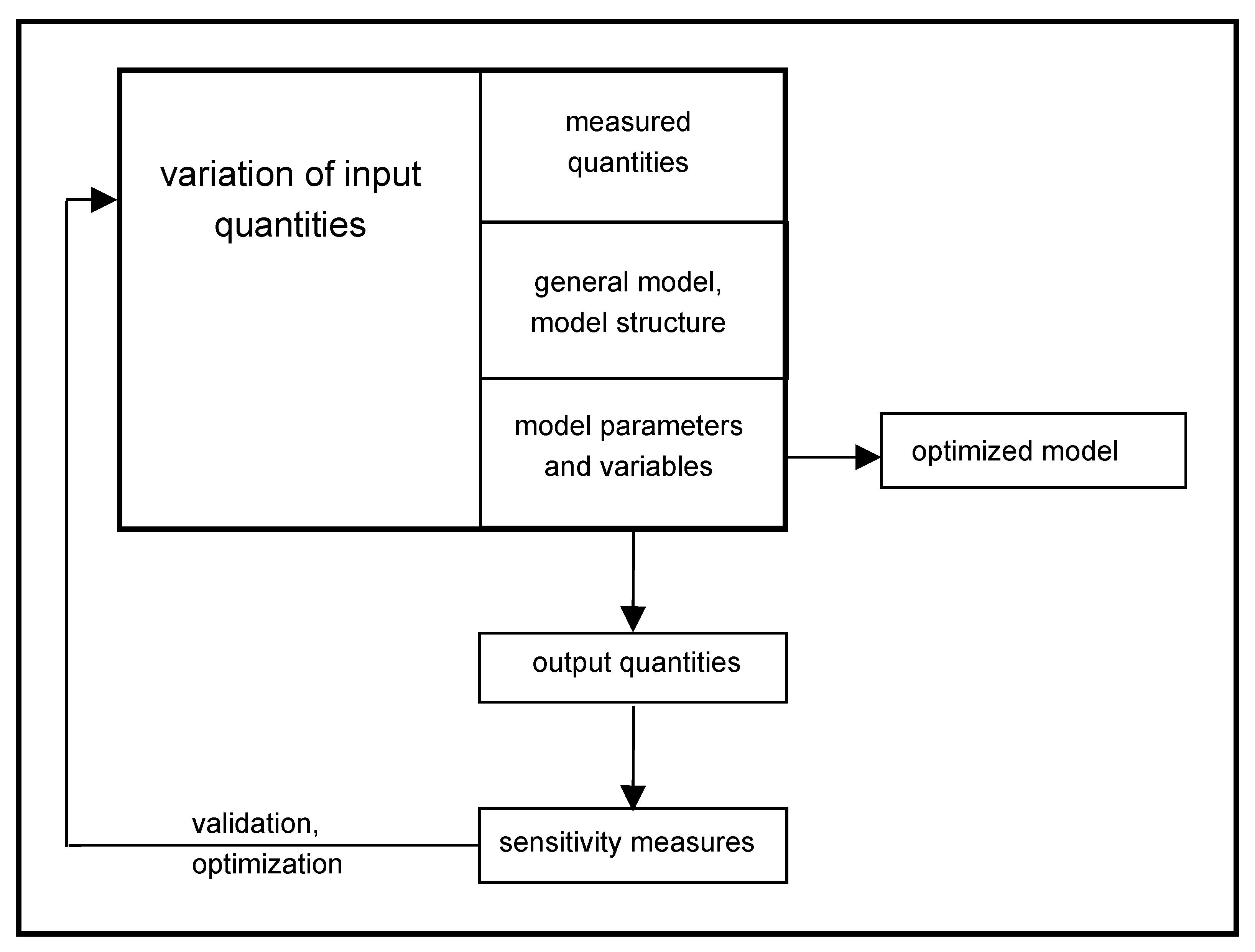
Definition 1.

SA is the study of how the variation in the output values of a model can be distributed among the different sources of variation among the input parameters.“ SA consists of the following stages [24,25]:

• define the model and its input and output parameters,
• determine the corresponding density functions for each input parameter,
• generate the so-called “input matrix” of values with an appropriate random sample generation method,
• compute the model output based on the generated values,
• analyze the fluctuations in the model output,
• estimate the influence (or relative importance) of the input parameters on the fluctuations in the output.

There are various approaches available for conducting sensitivity analysis (SA), as referenced in [29]. The choice of SA method depends on the behavior of the model, including factors such as linearity, monotonicity, and additivity in the relationship between input parameters and output.

SA can be divided into two distinct classes: local and global. Local SA focuses on understanding how small changes in values around a fixed point impact the variability of output values. This method involves investigating the sensitivity of individual parameters while keeping other parameters constant and only allowing the selected parameter to vary. It is commonly known as the “one at a time” (OAT) technique. However, OAT experiments do not consider the joint influence of multiple parameters. On the other hand, global SA examines the entire range of variation in input parameter values. Parameter screening methods, such as the ones discussed in [35], are specifically designed for models with a large number of input parameters or those that pose estimation challenges. Although these methods are useful for sensitivity analysis, they have a key limitation. They provide a qualitative estimation of sensitivity by grouping input parameters based on their influence, but they do not provide a quantitative measure of the individual importance of each parameter in relation to the others.

Variance-based methods (VBM) are widely used quantitative techniques for SA [25]. These methods employ random samples and are particularly suitable for MC simulations. Input parameters are modeled as random variables characterized by probability density functions. The main objective of VBM is to identify the input parameters that have the most significant impact on output variations and determine which parameters require more accurate estimation to reduce uncertainties in output values.

When conducting a detailed analysis of concentration sensitivities in large mathematical models, it is beneficial to introduce stochastic variables and equations. Sobol’s work in [36] provides a successful systematic framework for this theory.

Let the mathematical model be represented by a model function

$$\mathrm{u}=f\left(\mathrm{x}\right),\mathrm{where}\mathrm{x}=(x_1,x_2,\dots ,x_d)\in U^d\equiv {[0;1]}^d$$

(1)

is a vector of input parameters with joint probability density $p\left(\mathrm{x}\right)=p(x_1,\dots ,x_d)$. We assume that the output is a scalar and that the input parameters are independent and the probability density $p\left(\mathrm{x}\right)=p(x_1,x_2,\dots ,x_d)$ is known. Therefore, the output parameter $\mathrm{u}$ is a random variable as a function of the random vector $\mathrm{x}$.

We now introduce the measure of the degree of influence of an input parameter on the output.

Definition 2.

(First-order sensitivity index [37])The basic indicator corresponding to a given input parameter $x_i,i=1,\dots ,d$ (normalized between 0 and 1) is called the Sobol first-order sensitivity index (SI) [37] and is defined as follows

$${\displaystyle \frac{\mathbf{D}\left[\mathbf{E}\left[\mathrm{u}\right|x_i]\right]}{{\mathbf{D}}_{\mathrm{u}}},}$$

(2)

where $\mathbf{D}\left[\mathbf{E}\left[\mathrm{u}\right|x_i]\right]$ is the variance of the conditional mathematical expectation of $\mathrm{u}$ on $x_i$, and ${\mathbf{D}}_{\mathrm{u}}$ is the full variance on $\mathrm{u}$.

We now give a definition of the total SI.

Definition 3.

Total sensitivity index (TSI) [27] is a measure of the overall influence (full effect) of an input parameter on variations in the output. The TSI of the input parameter $x_i,x_i\in 1,\dots ,d$ is defined as follows [27,37]:

$${\displaystyle S_{x_i}^{tot}=S_i+\sum _{l_1\ne i}{S}_{i{l}_1}+\sum _{l_1,l_2\ne i,l_1<l_2}{S}_{i{l}_1{l}_2}+\dots +S_{i{l}_1\dots l_{d-1}},}$$

(3)

where $S_i$ is called the main effect (first-order SI) of $x_i$ and $S_{i{l}_1\dots l_{j-1}}$ is the $j-th$-order SI (two-way interactions for $j=2$ and three-way interactions for $j=3$, etc.) for the parameter $x_i(2\le j\le d)$.

The degree of joint influence of the input parameters $x_{i_1},\dots ,x_{i_{\nu }},\nu \in \{2,\dots ,d\}$ on the variation of the result is described by the higher-order addends. In [38], it is shown that small subsets of the input parameters will contribute significantly to the output in multivariate models. Therefore, higher-dimensional adders can be neglected and lower-order SIs can be used, but the contribution of higher-order adders can be controlled.

The set of input parameters is classified depending on the TSI as $S_{x_i}^{tot}$ [24]: extremely important if $0.8<S_{x_i}^{tot}$, important if $0.5<S_{x_i}^{tot}<0.8$, unimportant if $0.3<S_{x_i}^{tot}<0.5$, and insignificant if $S_{x_i}^{tot}<0.3$.

We now consider one of the most commonly used VBMs, namely Sobol’s [36,37] method for computing global sensitivity indices (GSIs). The main advantage of this method is it computes not only first-order SIs but also higher-order SIs, and TSI can compute with only one integral (one subintegral function) for a given parameter by the MC method.

Sobol’s method for global SA relies on a decomposing the integrable model function f (in s-dimensional input parameter space) into addends of increasing dimensionality.

Definition 4.

The high-dimensional model representation (HDMR representation) is defined as

$$f\left(\mathrm{x}\right)=f_0+\sum _{\nu =1}^d\sum _{l_1<\dots <l_{\nu }}{f}_{l_1\dots l_{\nu }}(x_{l_1},x_{l_2},\dots ,x_{l_{\nu }}),$$

(4)

where $f_0$ is a constant. The total number of addends in Equation (4) is $2^d$ (see [39]).

In general, this representation is not unique to [37]. The key feature of (1) is that it can be represented by small subsets of input parameters [38,40], and this assumption is the basis of (4). Thus, functions on more variables describing the effect of the interaction of input parameters in (4) can be neglected. This will reduce the dimensionality of the problem.

Definition 5.

The representation (4) is unique and is called an ANOVA representation (analysis of variance, analysis of variance) of the model function $f\left(\mathrm{x}\right)$ [41], under the condition that for each additive is valid

$${\int }_0^1{f}_{l_1\dots l_{\nu }}(x_{l_1},x_{l_2},\dots ,x_{l_{\nu }})\mathrm{d}{x}_{l_k}=0,1\le k\le \nu ,\nu =1,\cdots ,d.$$

(5)

Sobol has proven [36] that the decomposition (4) is if and only if (5) holds and the functions on the right-hand side can be represented in a unique way [41]:

• ${\displaystyle f_0={\int }_{U^d}f\left(\mathrm{x}\right)\mathrm{d}\mathrm{x}}$;
• ${\displaystyle f_{l_1}\left(x_{l_1}\right)={\int }_{U^{d-1}}f\left(\mathrm{x}\right)\prod _{k\ne l_1}\mathrm{d}{\mathrm{x}}_k-f_0,l_1\in \{1,2,\dots ,d\}}$;
• $$\begin{gathered} {\displaystyle f_{l_1{l}_2}(x_{l_1},x_{l_2})={\int }_{U^{d-2}}f\left(\mathrm{x}\right)\prod _{k\ne l_1,l_2}\mathrm{d}{\mathrm{x}}_k-f_0-f_{l_1}\left(x_{l_1}\right)-f_{l_2}\left(x_{l_2}\right), \\ {l}_1,l_2\in \{1,2,\dots ,d\}.} \end{gathered}$$

Because the above subsets of indices differ from each other by at least one element and the corresponding integral is equal to zero for the corresponding index by applying (5), it follows that the addends in the ANOVA representation are mutually orthogonal

$${\displaystyle {\int }_{U^d}{f}_{i_1\dots i_{\mu }}{f}_{j_1\dots j_{\nu }}\mathrm{d}\mathrm{x}=0,(i_1,\dots ,i_{\mu })\ne (j_1,\dots ,j_{\nu }),\mu ,\nu \in \{1,\dots ,d\}.}$$

Definition 6.

The quantities

$${\displaystyle \mathbf{D}={\int }_{U^d}{f}^2\left(\mathrm{x}\right)\mathrm{d}\mathrm{x}-f_0^2,{\mathbf{D}}_{l_1\dots l_{\nu }}=\int f_{l_1\dots l_{\nu }}^2\mathrm{d}{x}_{l_1}\dots \mathrm{d}{x}_{l_{\nu }}}$$

(6)

are called variances (total and partial variances, respectively) and are obtained after squaring and integrating over $U^d$ the Equation (4) under the assumption that $f\left(\mathrm{x}\right)$ has a summable square.

Thus, we arrive at the following definition:

Definition 7.

The total variance of the model output parameter is decomposed into the partial variances [36] in an analogous way to the decomposition of the model function, which is only an ANOVA-type representation:

$$\mathbf{D}=\sum _{\nu =1}^d\sum _{l_1<\dots <l_{\nu }}{\mathbf{D}}_{l_1\dots l_{\nu }}.$$

(7)

It will now be shown how the corresponding SI $S_{l_1\dots l_{\nu }}$ are defined by the conditional expectation variances ${\mathbf{D}}_{l_1}=\mathbf{D}\left[f_{l_1}\left(x_{l_1}\right)\right]=\mathbf{D}\left[\mathbf{E}\left(\mathrm{u}\right|x_{l_1})\right]$, ${\mathbf{D}}_{l_1\dots l_{\nu }},2\le \nu \le d$ (see Equation (8)).

Definition 8

([36,41]). The quantities

$${\displaystyle S_{l_1\dots l_{nu}}=\frac{{\mathbf{D}}_{l_1\dots l_{nu}}}{\mathbf{D}},\nu \in \{1,\dots ,d\}}$$

(8)

are called Sobol GSIs.

This formula coincides with (2) for $\nu =1$, and so, the measures defined correspond to the main effect and the interaction effect between the parameters. Now, dividing (7) by $\mathbf{D}$, it follows that the following properties of these indices hold:

$${\displaystyle S_{l_1\dots l_{\nu }}\ge 0,\mathrm{and}\sum _{\nu =1}^d\sum _{l_1<\dots <l_{\nu }}^d{S}_{l_1\dots l_{\nu }}=1.}$$

Definition 9.

Let us have a set of m variables ($1\le m\le d-1$):

$$\mathrm{y}=(x_{k_1},\dots ,x_{k_m}),1\le k_1<\dots <k_m\le d,$$

and let $\mathrm{z}$ be the set of the remaining $d-m$ variables, $K=(k_1,\dots ,k_m)$, and $\mathrm{x}=(\mathrm{y},\mathrm{z})$. Then, the variances corresponding to the sets of variables $\mathrm{y}$ and $\mathrm{z}$ are defined as

$${\displaystyle {\mathbf{D}}_{\mathrm{y}}=\sum _{n=1}^m\sum _{(i_1<\dots <i_n)\in K}{\mathbf{D}}_{i_1\dots i_n},{\mathbf{D}}_z=\sum _{n=1}^{d-m}\sum _{(j_1<\dots <j_n)\in \overline{K}}{\mathbf{D}}_{j_1\dots j_n},}$$

(9)

where the complement of the subset K to the set of indices of all input parameters is denoted by $\overline{K}$, the first sum in (9) is over all subsets $(i_1,\dots ,i_n)$, where all indices $i_1,\dots ,i_n$ belong to K and the full variance of the subset $\mathrm{y}$−${\mathbf{D}}_{\mathrm{y}}^{tot}=\mathbf{D}-{\mathbf{D}}_{\mathrm{z}}$ is over all subsets $(i_1,\dots ,i_{\nu }),1\le \nu \le d$, where at least one index belongs to K: $i_l\in K,1\le l\le \nu$.

The procedure for calculating the GSI is based on the following representation of the variance ${\mathbf{D}}_{\mathrm{y}}$: ${\displaystyle {\mathbf{D}}_{\mathrm{y}}=\int f\left(\mathrm{x}\right)f(\mathrm{y},{\mathrm{z}}^{\prime })\mathrm{d}\mathrm{x}\mathrm{d}{\mathrm{z}}^{\prime }-f_0^2}$ (see [41]). The last equality allows for the construction of an MC algorithm to compute $f_0,\mathbf{D}$ and ${\mathbf{D}}_{\mathrm{y}}$, where $\xi =(\eta ,\zeta )$:

$$\begin{array}{cc}{\displaystyle \frac{1}{N}\sum _{j=1}^{N}f\left({\xi }_j\right)\stackrel{P}{⟶}{f}_0,}\hfill & {\displaystyle \frac{1}{N}\sum _{j=1}^{N}f\left({\xi }_j\right)f({\eta }_j,{\zeta }_j^{\prime })\stackrel{P}{⟶}{\mathbf{D}}_{\mathrm{y}}+f_0^2,}\hfill \\ {\displaystyle \frac{1}{N}\sum _{j=1}^N{f}^2\left({\xi }_j\right)\stackrel{P}{⟶}\mathbf{D}+f_0^2,}\hfill & {\displaystyle \frac{1}{N}\sum _{j=1}^{N}f\left({\xi }_j\right)f({\eta }_j^{\prime },{\zeta }_j)\stackrel{P}{⟶}{\mathbf{D}}_{\mathrm{z}}+f_0^2.}\hfill \end{array}$$

Therefore, for $m=1,\mathrm{y}=\left\{x_{l_1}\right\},l_1\in \{1,\dots ,d\}$ and $\mathrm{z}=\{1,\dots ,d\}\setminus l_1$:

$${\displaystyle S_{l_1}=S_{\left(l_1\right)}=\frac{{\mathbf{D}}_{\left(l_1\right)}}{\mathbf{D}},S_{l_1}^{tot}=\frac{{\mathbf{D}}_{l_1}^{tot}}{\mathbf{D}}=1-S_{\mathrm{z}}.}$$

Following the idea of Homa and Saltelli in [27], a better first-order approximation of SI is obtained if $f_0^2$ in (6) is approximated directly using

$${\displaystyle f_0^2={\int }_{U^{2d}}f\left(\mathrm{x}\right)f\left({\mathrm{x}}^{\prime }\right)\mathrm{d}\mathrm{x}\mathrm{d}{\mathrm{x}}^{\prime }}$$

instead of ${\displaystyle f_0^2={\left[{\int }_{U^d}f\left(\mathrm{x}\right)\mathrm{d}\mathrm{x}\right]}^2}$. This follows from the Formula (6), where the corresponding estimate of the first-order indices $S_{l_1},l_1\in \{1,\dots ,d\}$ tends to zero for the corresponding input parameter $x_{l_1}$ if () [30] is used and can be obtained from the formula:

$${\displaystyle D_{l_1}={\int }_{U^{2d}}f\left(\mathrm{x}\right)[f(x_1^{\prime },\dots ,x_{l_1-1}^{\prime },x_{l_1},x_{l_1+1}^{\prime },\dots ,x_d^{\prime })-f(x_1^{\prime },\dots ,x_d^{\prime })]\mathrm{d}\mathrm{x}\mathrm{d}{\mathrm{x}}^{\prime }.}$$

Saltelli’s idea in [30] for computing TSI is to use the following estimate for $S_{l_1}^{tot}$:

$${\displaystyle 1-\frac{1}{\mathbf{D}}\left\{{\int }_{U^{d+1}}f(x_1,\dots ,x_d)f(x_1,\dots ,x_{l_1-1},x_{l_1}^{\prime },x_{l_1+1},\dots ,x_d)\mathrm{d}\mathrm{x}\mathrm{d}{\mathrm{x}}_{l_1}^{\prime }-f_0^2\right\}.}$$

The computational complexity of the aforementioned method for computing all first-order SIs and all TSIs is determined by the number of function evaluations required, which is proportional to $N(2d+1)$ (N values of the function for $f_0$, $dN$ values of the SIs function, and $dN$ values of the TSIs function), where N represents the sample size and d is the number of dimensions.

In contrast, commonly used VBMs such as Sobol’s method and FAST have a computational complexity that scales linearly with $dN$ when estimating all first-order SIs and TSIs for the input parameters (see [30]).

This illustrates that the core of the SA problem resides on the computation of TSIs (3) and, more specifically, the Sobol GSIs of the corresponding order (8). This computation can be reduced to the evaluation of multidimensional integrals:

$$I={\int }_{\Omega }g\left(\mathrm{x}\right)p\left(\mathrm{x}\right)\mathrm{d}\mathrm{x},\Omega \subset {\mathbb{R}}^d,$$

where $g\left(\mathrm{x}\right)$ is a summable square function in $\Omega$ and $p\left(\mathrm{x}\right)\ge 0$ is a probability density, such that ${\int }_{\Omega }p\left(\mathrm{x}\right)\mathrm{d}\mathrm{x}=1$.

Consequently, we observe that the computation of the $2^d$ integrals of the form (6) is necessary to obtain the TSI $S_{x_i}^{tot}$ for a fixed parameter.

The whole methodology for performing SA is given on Figure 1.

3. Mathematical Model UNI-DEM

Ongoing research and computational experiments have been conducted utilizing the unified Danish Euler model (UNI-DEM), also known as UNI-DEM, which has proven to be a robust mathematical framework for accurately capturing the relevant physical and chemical processes [8,9,10,42]. The integration of the unified Danish Eulerian model (UNI-DEM) with various suitable climatic scenarios holds a pivotal and highly significant position within the framework of DIGITAL AIR. Developed by Prof. Zahari Zlatev and their colleagues at the Danish National Institute for Environmental Research [9], UNI-DEM possesses the ability to effectively calculate the concentrations of various hazardous pollutants. It has been widely employed for over two decades in interdisciplinary research and long-term simulations addressing air pollution. Importantly, the proposed SA methodology can be readily extended to other models, showcasing its versatility and applicability beyond UNI-DEM.

UNI-DEM serves as a simulation tool for studying the long-range transport of air pollutants, their temporal changes resulting from chemical and photochemical reactions, and their interactions with the environment. It incorporates crucial physical processes such as advection, diffusion, deposition, emissions, and chemical transformations. The model allows for the analysis of pollutant concentrations over time, specifically focusing on sulfur, nitrogen, ammonia, ammonium ions, nitrogen radicals, and hydrocarbons, which have significant implications for environmental, agricultural, and public health concerns. The geographic scope of the model encompasses Europe, the Mediterranean, and parts of Asia and Africa, with an approximate area coverage of $4800\times 4800$ km.

To effectively handle the complexity of the model, it is divided into three subsystems or submodels, each targeting specific physical and chemical processes. By discretizing these submodels and utilizing parallel computing on powerful supercomputers, the model can be executed efficiently in real-time, enabling practical problem-solving within reasonable timeframes [8,9].

Chemical reactions play a pivotal role in the model [43]. The equations within the model accurately represent the system by accounting for chemical reactions. The presence of these reactions contributes to the nonlinearity and “rigidity” of the equation system [43]. The model employs the compressed CBM-IV (carbon bond mechanism) chemical scheme, which has been enhanced in [8]. It encompasses 35 pollutants and 116 chemical reactions, with 69 reactions being time-dependent and 47 being time-independent. This chemical scheme is well-suited for investigating scenarios involving high pollutant concentrations.

Among the model components, chemical reactions are the most challenging and time-consuming, with 69 time-dependent and 47 time-independent reactions requiring careful consideration.

The rate constant in chemical reactions signifies the reaction rate when reactant concentrations are at 1 mol/L, as described by the law of mass action discovered by Guldberg and Waage [30]. Therefore, the intensity of the chemical rate constant directly influences the rate of chemical processes.

The model is described mathematically by [8,10,31] through the following system of partial differential equations:

$$\begin{array}{ccc}\hfill {\displaystyle \frac{\partial c_s}{\partial t}}& =& {\displaystyle -\frac{\partial \left(u{c}_s\right)}{\partial x}-\frac{\partial \left(v{c}_s\right)}{\partial y}-\frac{\partial \left(w{c}_s\right)}{\partial z}+}\hfill \\ & & {\displaystyle +\frac{\partial }{\partial x}\left(K_x\frac{\partial c_s}{\partial x}\right)+\frac{\partial }{\partial y}\left(K_y\frac{\partial c_s}{\partial y}\right)+\frac{\partial }{\partial z}\left(K_z\frac{\partial c_s}{\partial z}\right)+}\hfill \\ & & {\displaystyle +E_s+Q_s(c_1,c_2,\dots ,c_q)-(k_{1s}+k_{2s})c_s,s=1,2,\dots ,q.}\hfill \end{array}$$

(10)

The number q of equations in (10) is equal to the number of pollutants that are studied by the model. The other quantities included in the model are described below:

• $c_s$—the pollutant concentrations,
• $u,v,w$—the wind components along the coordinate axes,
• $K_x,K_y,K_z$—diffusion coefficients,
• $E_s$—the emission in the spatial domain,
• $k_{1s},k_{2s}$—the dry and wet deposition coefficients, respectively, ($s=1,\dots ,q$),
• $Q_s(c_1,c_2,\dots ,c_q)$—nonlinear functions describing chemical reactions between pollutants.

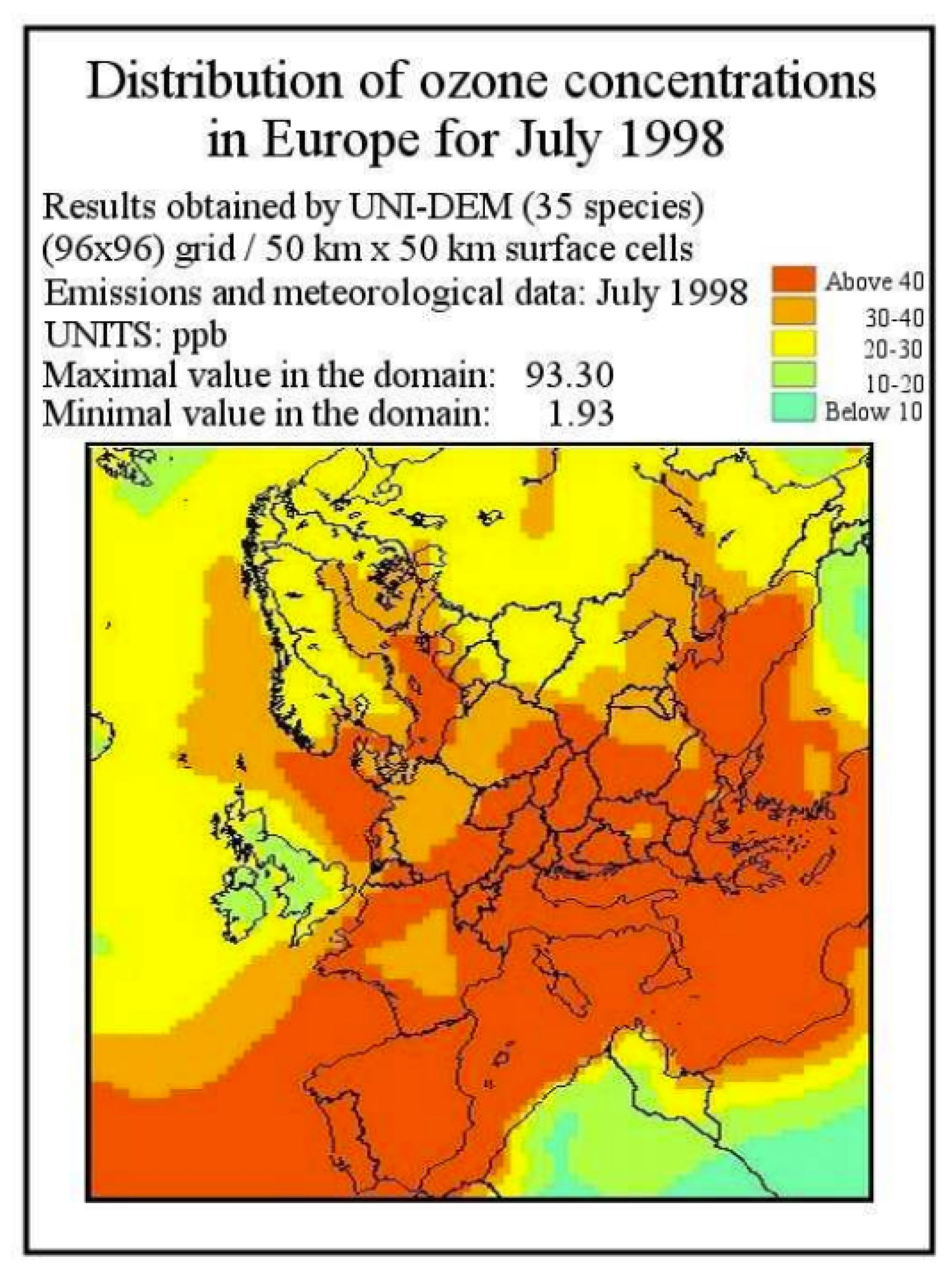
The region of study and the computational domain is shown on Figure 2.

The UNI-DEM spatial domain, utilizing a stereographic geographic projection, comprises a surface plane that measures (4800 km × 4800 km). This plane encompasses Europe and its surrounding regions. Each of the ten horizontal levels is discretized using a grid with dimensions of (10 km × 10 km). This discretization ensures an ample number of cells, accommodating even small European countries such as Denmark and Bulgaria [10].

The same spatial domain was discretized into a $480\times 480$ grid with a resolution of 10 × 10 km. Although this refinement significantly increases computational requirements, the comparison between results obtained on the coarse and fine grids demonstrates the value of these efforts, particularly when utilizing the 3-D versions with 10 non-equidistant layers in the vertical direction. However, it was not feasible to acquire input data, including emission and meteorological data, at this high-resolution grid. Instead, the available emission data on the 50 km grid were evenly distributed across 25 smaller grid squares obtained during the transition to the 10 km resolution. To prepare meteorological data for the fine grid, simple linear interpolation is employed, both spatially and temporally.

At the surface level, there are a total of $230,400$ grid squares, each measuring (10 km × 10 km). The model typically runs with a time step of 30 s, spanning a continuous period of 16 years [31].

Several conditions specified in [8] are assumed. Firstly, the spatial derivatives in the system of PDEs (10) are directly discretized. Secondly, the first-order backward differentiation formula is applied to solve the resulting system of ODEs that arise from the discretization of spatial derivatives. Thirdly, the chosen chemical scheme is the CBM-IV scheme, involving 56 chemical species. Finally, the model is executed for a duration of 16 years.

Under these assumptions, each time step requires the processing of $3600/30\times 24\times 365\times 16=16,819,200$ sets of nonlinear algebraic equations. Each of these sets contains $480\times 480\times 10\times 56=129,024,000$ equations. To solve these nonlinear algebraic equations, iterative methods are employed, resulting in the solution of very large systems of linear algebraic equations within an inner loop at each time step. The number of these systems during a one-year loop is estimated to be substantial, approximately $O\left({10}^9\right)$ or even higher.

The UNI-DEM, within the context of DIGITAL AIR, was executed using a total of 14 distinct scenarios spanning a continuous period of 16 years from 1989 to 2004. These scenarios encompass various conditions and factors. The first among the selected five scenarios served as the baseline, providing a reference point for comparison. The subsequent three scenarios were constructed based on assumptions regarding future temperature increases, derived from the conclusions drawn in the IPCC report. The fifth scenario incorporated an additional aspect, considering the anticipated rise in natural emissions of certain air pollutants. 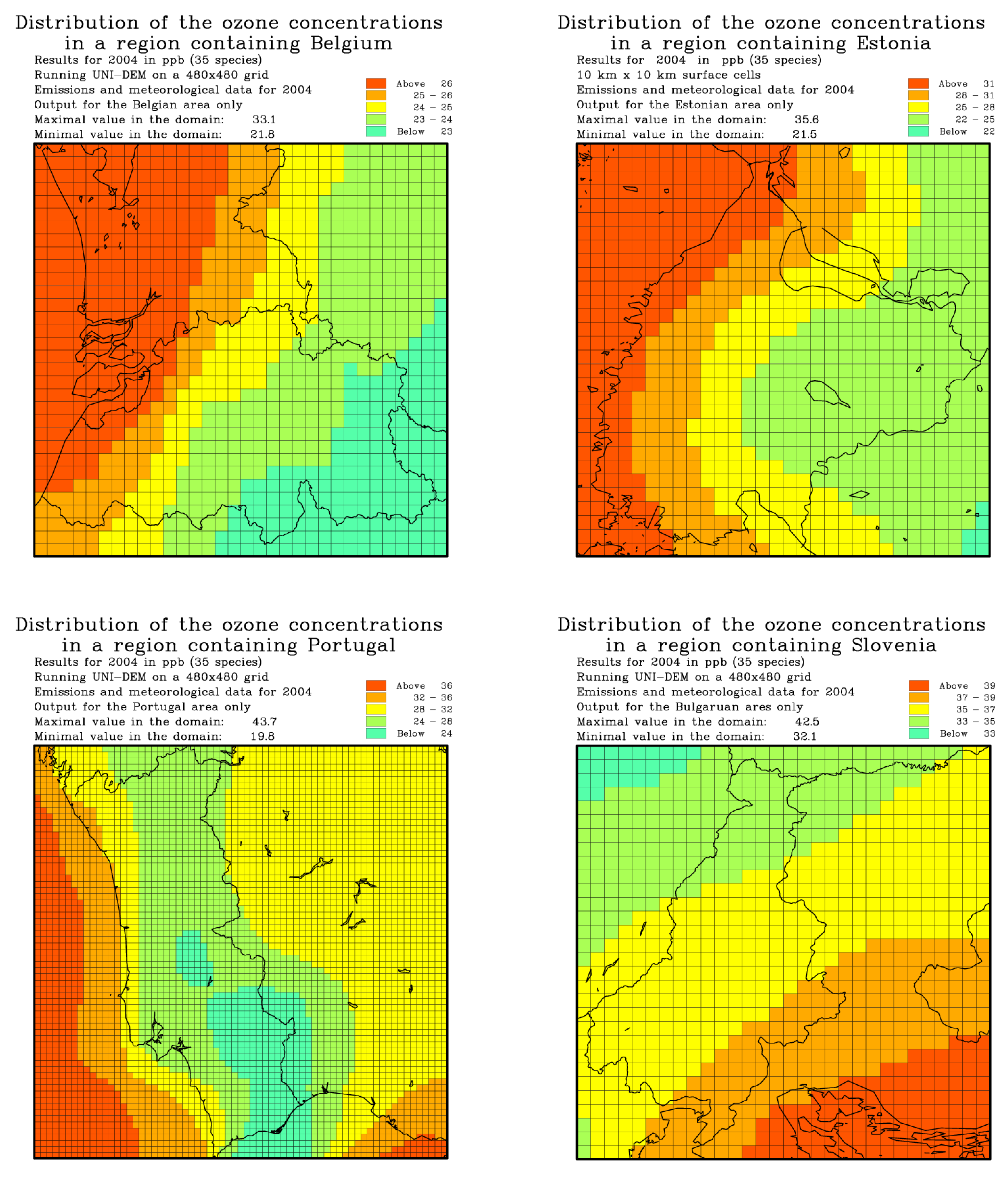Figure 3 illustrates the capability of UNI-DEM to generate dependable outcomes even for the smaller countries in Europe.

The baseline scenario uses actual meteorological data and actual emissions data in Europe and its surroundings over the selected period of 16 consecutive years (1989 to 2004), whose data are obtained from the EMEP (European Monitoring and Evaluation Programme) database (for detailed information on the Basic scenarios and other scenarios in the digital twin, see [7]).

The definitions presented in [7] outline the First Climate Scenario, which focuses solely on changes in temperature. To visualize the anticipated temperature patterns in Europe, the scenario employs annual temperature changes recommended in various IPCC specialist reports [44]. These changes are used to create a map representing future temperature expectations for the first horizontal level of the digital twin’s spatial domain, known as UNI-DEM. This level consists of a grid with dimensions of $(480\times 480)$ cells. The study in [7] reveals that the mean annual temperature change within each cell of the first horizontal level of UNI-DEM corresponds to the prescribed values from the IPCC reports for each of the selected 16 years. The approach adopted in [7] assumes that the expected temperature increase in a particular cell during a given hour between 1989 and 2004 falls within the range of $[a,b]$. It is demonstrated that the temperature in this cell at a specific hour experiences an increase in $a+\gamma \left(n\right)$, where $\gamma \left(n\right)$ is a randomly generated and uniformly distributed quantity in the interval $[0,b-a]$. Consequently, the mathematical expectation of the average annual temperature increase in any cell within the first level of the spatial domain, across any year within the 16-year interval, is equal to $(b-a)/2$.

Based on the conclusions derived from the IPCC reports, it is projected that extreme events will intensify in the future. Specifically, the Second Climate Scenario, which was analyzed, indicates that maximum daily temperatures will rise, leading to an increased frequency of hot days in terrestrial areas. Additionally, a majority of land regions will experience elevated minimum temperatures, fewer occurrences of cold days, and a decrease in frosty days. Moreover, the diurnal temperature range will shrink in terrestrial regions. These anticipated changes have been taken into consideration in the Second Climate Scenario, and although it incorporates temperature variations similar to those in the First Climate Scenario, it introduces two additional modifications. Firstly, nighttime temperatures are increased by a greater proportion in comparison to daytime temperatures. Secondly, during summer periods, hotter days experience a larger temperature increase.

The Third Climate Scenario, which is the most advanced of the three scenarios, incorporates further findings from the IPCC experts. This scenario expands upon the Second Climate Scenario by considering the following conclusions: increased winter precipitation across land and water, reduced precipitation in continental Europe, adjustments in humidity data, a 10% increase in winter cloud cover, and maintaining the same cloud cover as the Second Climate Scenario during summer. The expected average annual temperature changes remain unchanged. Notably, the Third Climate Scenario is the only one visualized in [7].

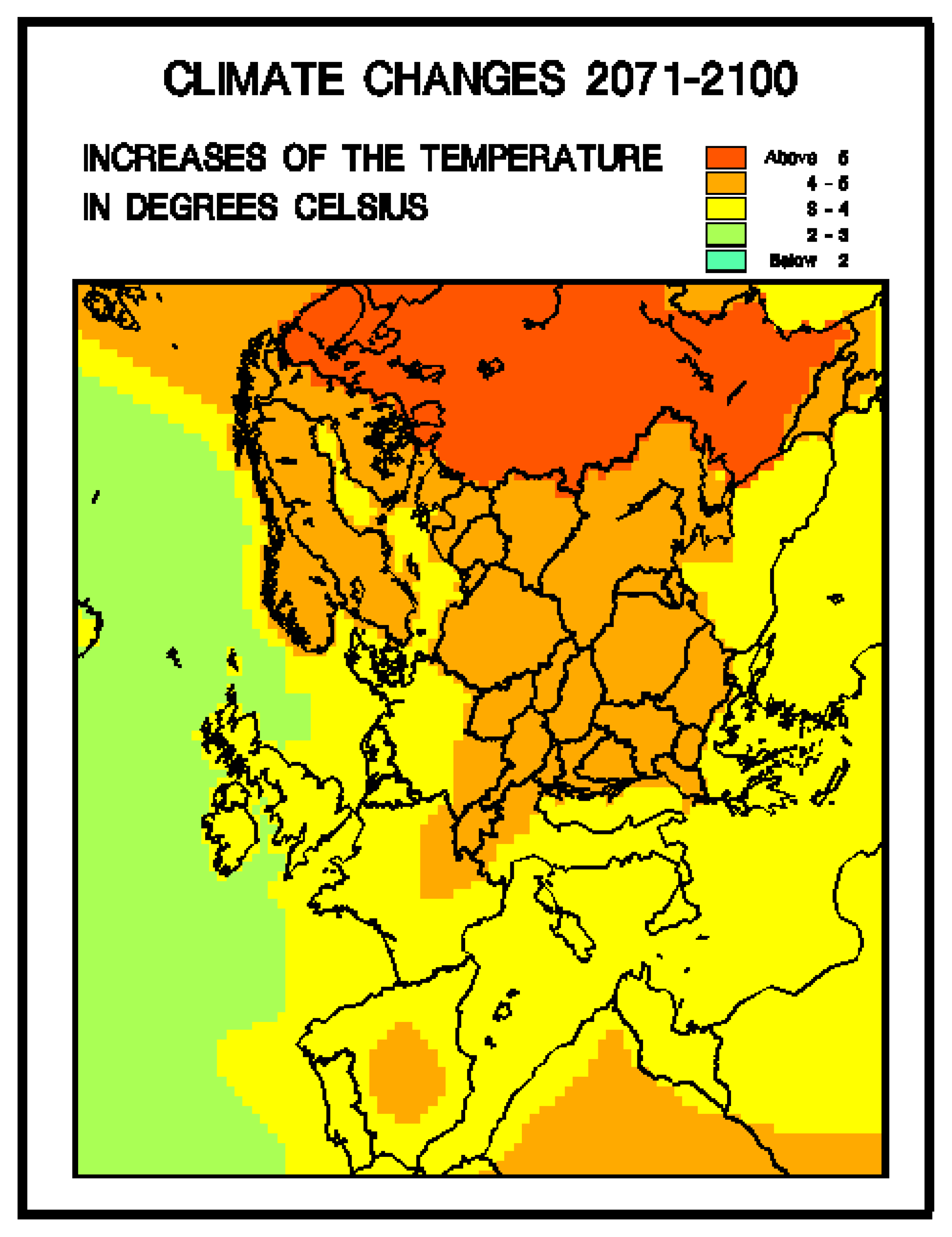
The significance of natural (biological) emissions is progressively growing and emerging as a crucial factor. There are at least two underlying factors contributing to this rise. Firstly, there has been a continuous reduction in human-made (anthropogenic) emissions in numerous European countries over the past two to three decades. Secondly, anticipated climatic changes and elevated temperatures are expected to stimulate an increase in natural (biological) emissions. Consequently, it is valuable to develop and implement scenarios incorporating higher natural (biological) emissions. Several scenarios incorporating recommended adjustments to the magnitude of biological (natural) emissions, are employed to address this objective in [7,45,46]. Anticipated temperature rises within the initial horizontal level of the UNI-DEM spatial domain as indicated by the findings of the IPCC reports are shown on Figure 4.

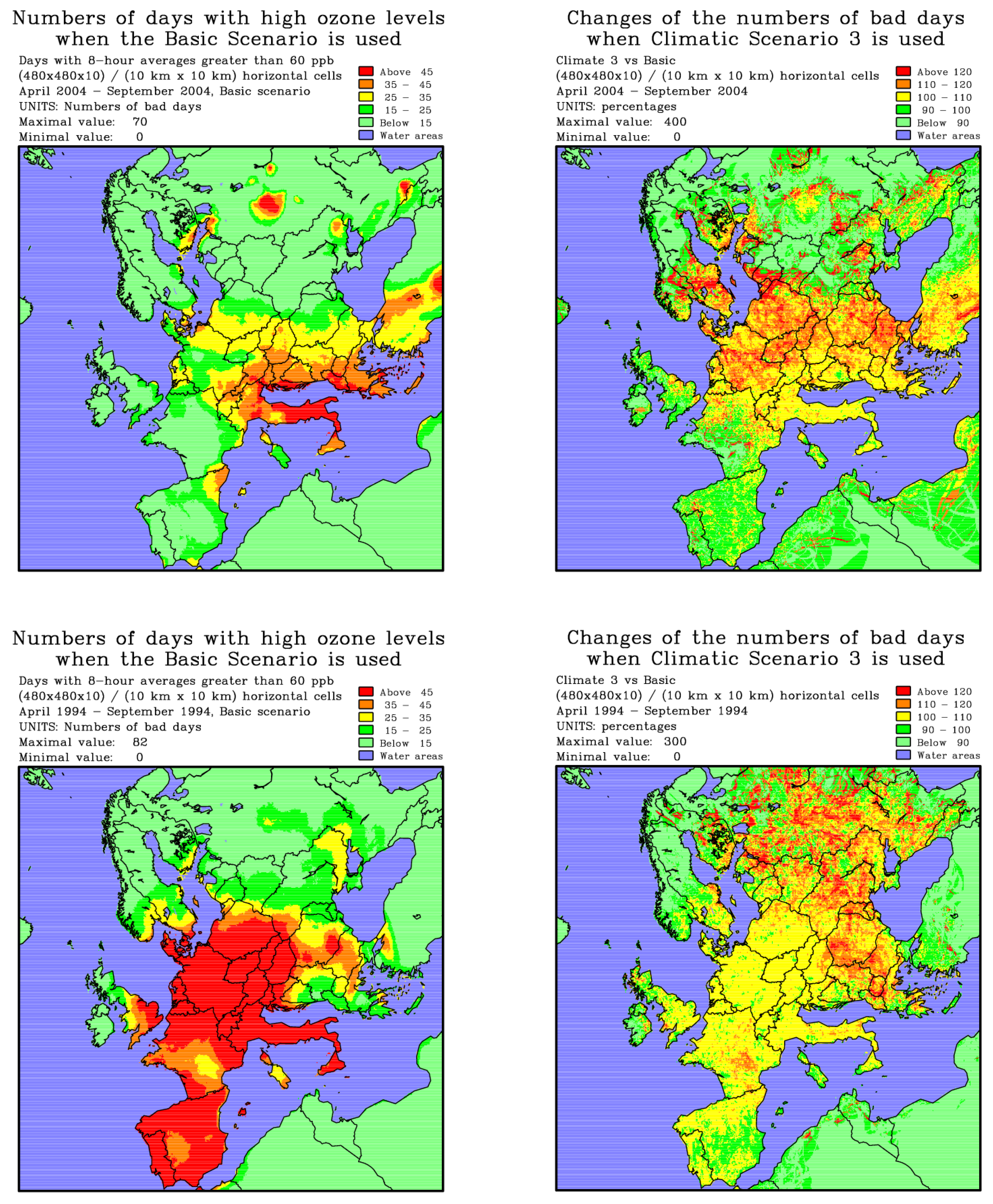
The subsequent analysis will delve into the outcomes obtained across the entire domain of UNI-DEM using the climatic scenarios discussed earlier. Our primary focus will be on evaluating the ozone levels not only throughout Europe but also in specific cities within the region. Of particular concern are instances of high ozone concentrations, as they can have detrimental effects, especially on vulnerable groups such as individuals with respiratory conditions such as asthma. Therefore, we will present detailed findings regarding the extent of these concentrations in various parts of Europe. Specifically, our investigation centers around identifying the occurrence of “bad days”. To qualify as a “bad day”, we examine the maximum value, denoted as $c_{m}ax$, of the 8 h average ozone concentrations at a given location in Europe on any given day. If $c_{m}ax$ exceeds 60 ppb at least once during that day, it is categorized as a “bad day”. It is imperative to ensure that the number of “bad days” remains within acceptable limits, preferably not exceeding 25 per year as recommended in the Ozone Directive issued by the EU Parliament in 2002.

Figure 5 provides visual representations illustrating the distribution of “bad days” throughout Europe. The distribution and frequency of “bad days” in different regions of Europe exhibit significant variability from year to year, as evident in the two left-hand side plots, which depict results from the Basic Scenario for the years 1994 and 2004. Implementation of the Third Climatic Scenario generally leads to an increase in the occurrence of “bad days.” The magnitude of these changes can be substantial, as indicated in the plots on the right, which present the percentage increases in the number of “bad days” for the selected years. Across numerous parts of Europe, the number of “bad days” exceeds the recommended limit of 25 days, demonstrating a considerable level of exceedance.

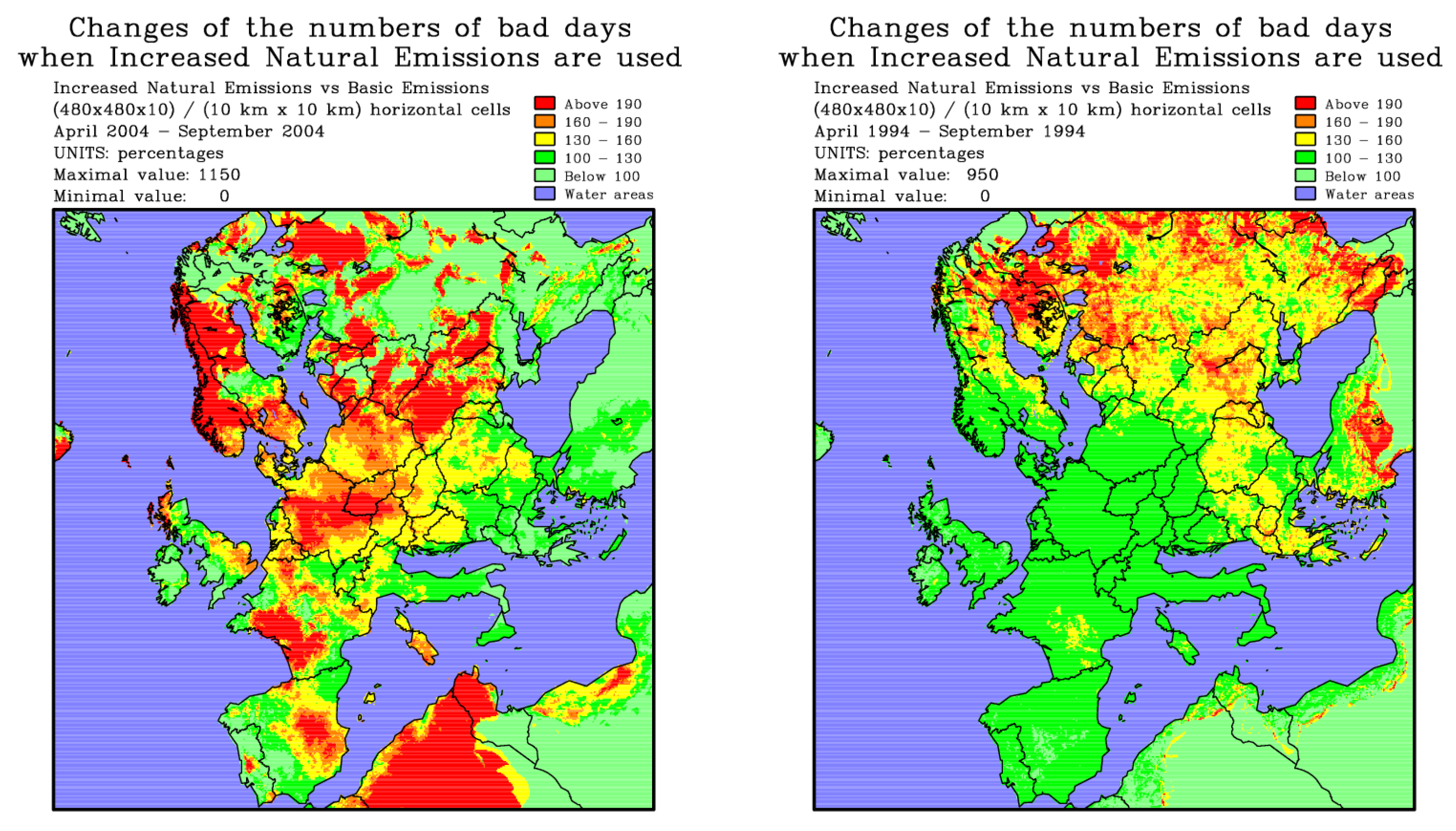
Figure 6 presents certain outcomes obtained in the surface domain of UNI-DEM by utilizing the impact of natural (biogenic) emissions on ozone levels in Europe. The two plots reveal significant variations across different regions of Europe and from one year to another. These changes can be substantial and exhibit distinct patterns. Overall, there is a consistent trend observed wherein the increase in biogenic (natural) emissions results in a substantial rise in the frequency of “bad days” across numerous parts of Europe.

4. Preliminary Calculations with UNI-DEM

By definition, SA includes models, input parameters, and output parameters. In this study, anthropogenic emissions and chemical reaction rate constants are considered as input parameters and pollutant concentrations as output parameters. Mathematically, the input parameters are treated as normally distributed random variables (which is established in [10]) whose mathematical expectation is $1.0$. The spatial domain of UNI-DEM is discretized by $96\times 96\times 10$ nodes in the three-dimensional version of UNI-DEM.

UNI-DEM experiments were conducted for the period 1994–1998. It is important to pay attention to the fact that a specific year is less important in climate research, because it takes about 30 years to change the climate scenario. The season of the year and the region for which the corresponding climate study was made are much more important. Therefore, a relatively long period in the past was chosen to allow us to compare the results for the data produced by the digital twin with the actual measured pollution data in that period. Furthermore, this comparison shows a high (and previously estimated precision of the digital twin) precision.

The (10) was considered leaving only the adders describing the emissions and chemical reactions. As they do not depend on spatial variables, (10) is reduced to a system of ODEs

$$d{g}_{s,i,j,k}/dt=E_{s,i,j,k}+Q_{s,i,j,k}(g_{1,i,j,k},g_{2,i,j,k},\dots ,g_{q,i,j,k}),$$

(11)

where $g_{s,i,j,k}\left(t\right)$ is the concentration value $c_s$ at the point $(x_i,y_j,z_k)$ of the grid at time t.

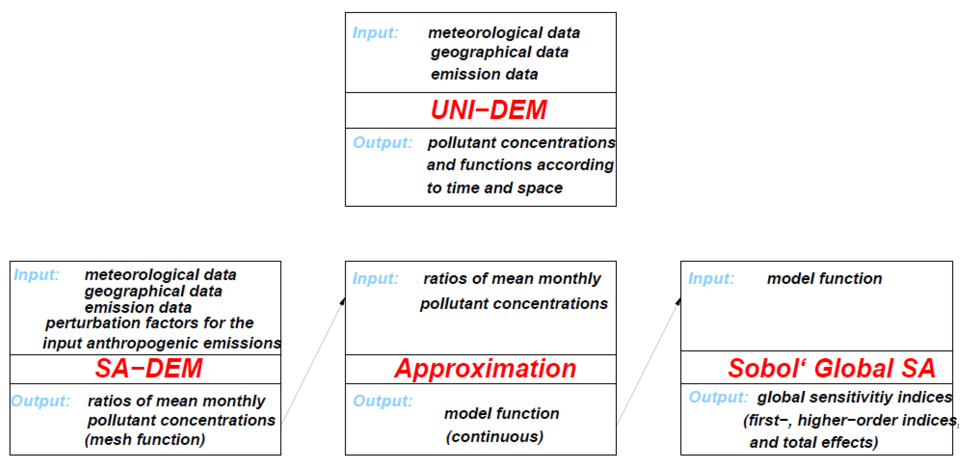
The different stages and components of the SA scheme for UNI-DEM (SA-DEM) is given in Figure 7.

The UNI-DEM model is employed at a fixed location within the mesh, and a smaller system known as the “box model” [10] is utilized for sensitivity analysis purposes. The box model represents a reduced system that can be solved repeatedly without computational difficulties, unlike the entire model, which involves solving large systems of ODEs at each time step and can be computationally challenging due to its size (containing millions of equations). In the sensitivity studies, the box model is solved multiple times while varying the rate constants of chemical reactions using a perturbation parameter $\alpha$, where $\alpha \in 0.1,0.2,\dots ,2.0$. Through this computational procedure, it was observed that the concentrations of pollutants are primarily sensitive to changes in the rate constants of the third and twenty-second time-dependent reactions, as well as a sixth time-independent reaction. These initial findings guided the subsequent comprehensive SA employing the aforementioned approaches to obtain more accurate and precise results.

In previous studies [47,48], the identification of critical rate constants of chemical reactions based on a specific criterion was performed. Ozone, known as a highly hazardous air pollutant, was the focus of investigation. The analysis focused on the average concentrations of ozone ($O_3$) during the summer month of July because it is recognized as the period with the highest ozone concentration.

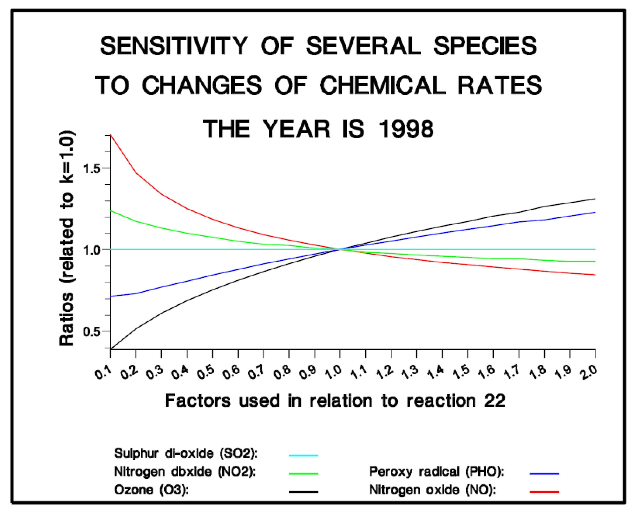
By iteratively solving the system defined by (10) while varying the rate constants of chemical reactions using a perturbation parameter $\alpha$ ranging from 0.1 to 2.0, the most influential rate constants were determined. Notably, the rate constant of the 22nd time-dependent chemical reaction was found to exert the most significant impact on the concentration of ozone ($O_3$). The effects of this specific rate constant on the concentrations of other pollutants, such as nitrogen dioxide ($N{O}_2$), sulfur dioxide ($S{O}_2$), peroxide radicals ($PHO$), and nitric oxide ($NO$), are illustrated in Figure 8. However, the influence on sulfur dioxide concentrations was practically negligible.

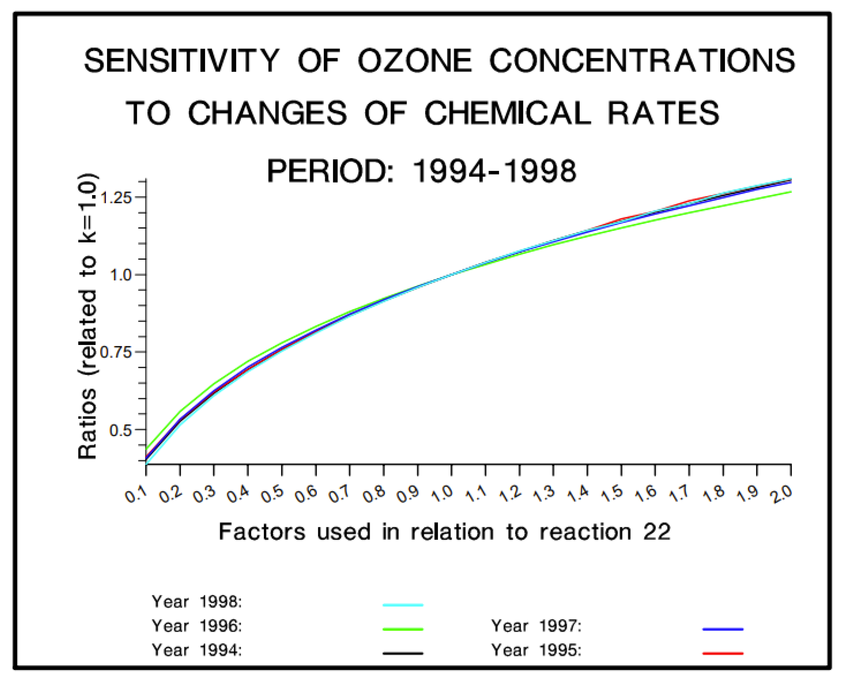
Furthermore, it was observed that the influence of the rate constant from the CMB IV chemical reaction on ozone concentration remained relatively consistent across different years. In other words, the pattern of concentration change in response to variations in the perturbation parameter showed a similar trend over time. This behavior is demonstrated in Figure 9.

It is also found that the concentrations of $O_3$ are most significantly affected by the following chemical reactions: $\#1,\#3,\#7$ (time-dependent) and $\#27,\#28$ (time-independent) reactions of CBM-IV ([8]). The simplified chemical equations of these reactions are as follows:

$$\begin{array}{cc}[\#\mathbf{1}]\hfill & N{O}_2+h\nu ⟹NO+O;\hfill \\ [\#\mathbf{3}]\hfill & O_3+NO⟹N{O}_2;\hfill \\ [\#\mathbf{7}]\hfill & N{O}_2+O_3⟹N{O}_3;\hfill \\ [\#\mathbf{22}]\hfill & H{O}_2+NO⟹OH+N{O}_2;\hfill \\ [\#\mathbf{27}]\hfill & H{O}_2+H{O}_2⟹H_2{O}_2;\hfill \\ [\#\mathbf{28}]\hfill & OH+CO⟹H{O}_2.\hfill \end{array}$$

Not all reactions involve ozone; instead, significant ozone precursors are involved. The UNI-DEM calculations primarily focus on obtaining the monthly average concentrations of various hazardous chemical species or groups of species. These concentrations are determined based on the specific chemical scheme and are calculated at grid points within the designated area. The input parameters in focus are the chemical reaction rates, whereas the output parameters of interest are the concentrations of pollutants.

To perform the UNI-DEM calculations, a set of perturbation parameters $\alpha =({\alpha }_1,\dots ,{\alpha }_6)$ is used within a six-dimensional hypercube ranging from 0.6 to 1.4. The values of $\alpha$ are chosen along the edges of the hypercube, starting from the vertex representing the Basic Scenario with true emissions and extending to all other vertices. Along each edge, the $\alpha$ samples are uniformly distributed by decrementing all variable coordinates by a fixed step of 0.1.

The generated data represent relationships of the form:

$${\displaystyle r_s\left(\alpha \right)=\frac{c_s^{\alpha }(a_s^{i_{max}},b_s^{j_{max}})}{c_s^{max}},{\alpha }_i\in \{0.1,0.2,\dots ,2.0\},}$$

where s corresponds to the contaminant (ranging from 1 to 35). The denominator $c_s^{max}$ represents the maximum average monthly value of pollutant concentration s without any perturbations, calculated at the coordinates $(a_s^{i_{max}},b_s^{j_{max}})$, and $i_{max},j_{max}$ are the grid indices of that point. The numerator represents the concentration value of the pollutant of interest for a specific set of perturbation parameter values ${\alpha }_i\in 0.1,\dots ,2.0$, calculated at the point $(a_s^{i_{max}},b_s^{j_{max}})$. Thus, the input data consist of pollutant concentrations normalized with respect to the maximum monthly mean value.

Before proceeding to the calculation of the Global Sensitivity Indices (GSIs) using Sobol’s method, an approximation is performed.

During the UNI-DEM calculations, tables of model function values are generated. These tables depict the relationship between ozone concentration values at fixed perturbation parameter values ${\alpha }_i\in 0.1,\dots ,2.0$, calculated at the point where the averaged maximum concentration is reached, and the corresponding averaged maximum for $\alpha =(1,\dots ,1)$. Because the sensitivity analysis assumes that the model is represented by a function as defined in Equation (1), the first step involves using an approximation technique to create a continuous function with analytically specified properties.

The approximation step using polynomials of different degrees was investigated. We utilize second-degree polynomials, characterized by 28 unknown coefficients, as a means of approximation. These polynomials, denoted as $p_s^{\left(k\right)}\left(\mathrm{x}\right)$, are employed to estimate the mesh function associated with the s-th chemical species:

$\begin{array}{cc}\hfill {\displaystyle p_s^{\left(k\right)}\left(\mathrm{x}\right)=\sum _{j=0}^k\sum _{({\nu }_1,{\nu }_2,\dots ,{\nu }_d)\in N_j^k}{a}_{{\nu }_1\dots {\nu }_d}{x}_1^{{\nu }_1}{x}_2^{{\nu }_2}\dots x_d^{{\nu }_d},k=2,}& \\ \hfill \mathrm{where}{N}_j^k=\left\{{\displaystyle ({\nu }_1,{\nu }_2,\dots ,{\nu }_d)|{\nu }_i=0,1,\dots ,k,\sum _{i=1}^d{\nu }_i=j}\right\}.\end{array}$

To evaluate the precision of the approximation, we employ the squared 2-vector norm. This norm, denoted as ${\displaystyle \Vert p_s-r_s{\Vert }_2^2=\sum _{l=1}^n{[p_s\left({\mathrm{x}}_l\right)-r_s\left({\mathrm{x}}_l\right)]}^2}$, is computed as the sum of squared differences between the values of the polynomial $p_s$ evaluated at specific points ${\mathrm{x}}_l$ and the corresponding table values $r_s\left({\mathrm{x}}_l\right)$. Here, ${\mathrm{x}}_l$ belongs to the interval ${[0.6;1.4]}^6$, and $r_s\left({\mathrm{x}}_l\right),l=1,\dots ,n$ represents the table values obtained from running the UNI-DEM model.

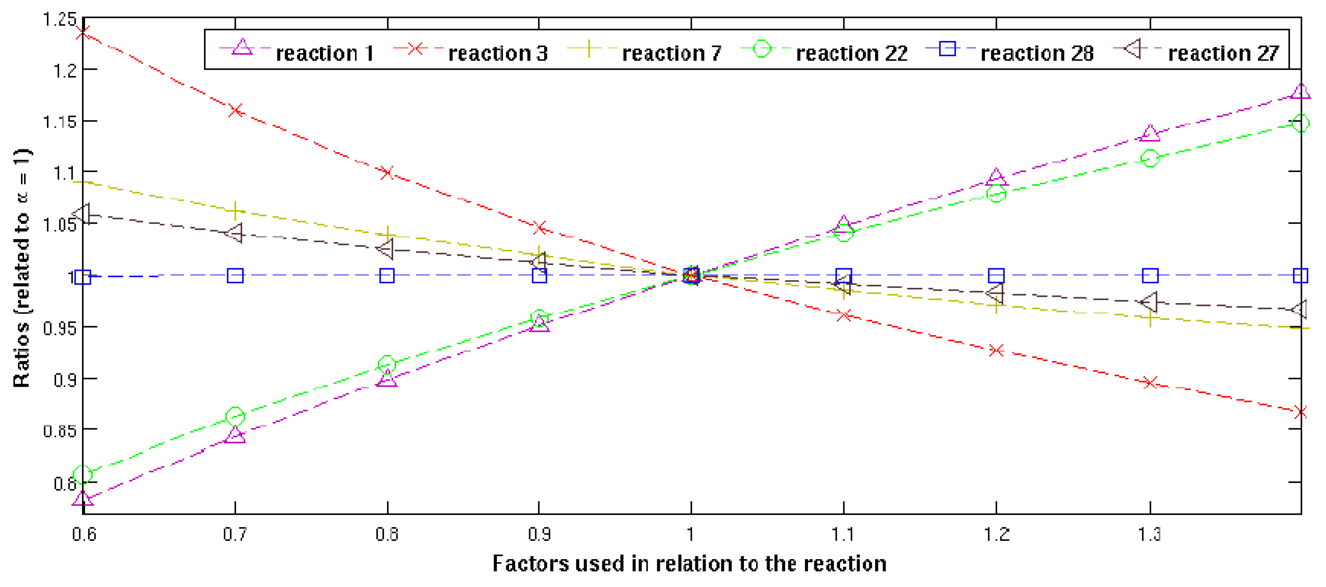
To examine the impact of different rate constants of chemical reactions on air pollution concentrations, a numerical investigation was conducted in [48]. Specifically, only one input value of the model was altered while keeping the others fixed at 1.0. 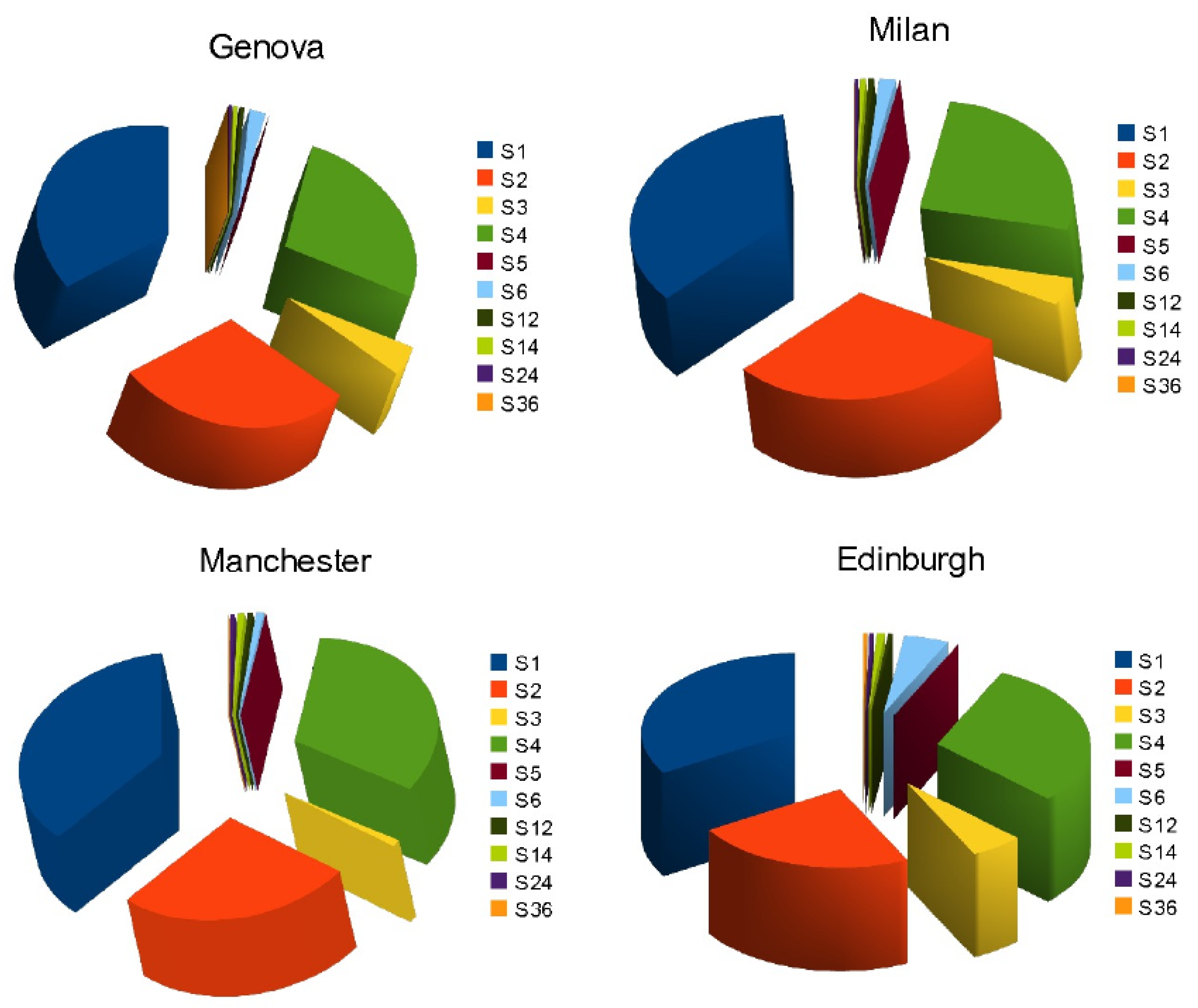The results analysis, focusing on the reactions considered by the CBM-IV scheme, revealed the following observations: the reaction rates $\#1,3,22$ exert a highly significant influence on the concentrations of thee ozone, whereas the impact of reaction rates and $\#7,27$, although less pronounced, remain significant. Conversely, the influence of reaction rate $\#28$ can be disregarded. The investigation of the impact of changes in chemical rates on ozone concentrations for Genova on July 1998 is given in Figure 10.

For the SA regarding input emissions, our focus is on examining the impact of perturbing anthropogenic emissions, given as input data, on the UNI-DEM output. Specifically, we study the sensitivity of monthly average ammonia concentrations in relation to these emissions perturbations.

The input data themselves consist of four different components $\mathbf{E}=({\mathbf{E}}^{\mathbf{A}},{\mathbf{E}}^{\mathbf{N}},{\mathbf{E}}^{\mathbf{S}},{\mathbf{E}}^{\mathbf{C}})$:

$$\begin{array}{cc}{\mathbf{E}}^{\mathbf{A}}-ammonia\left(N{H}_3\right);\hfill & {\mathbf{E}}^{\mathbf{S}}-sulfurdioxide\left(S{O}_2\right);\hfill \\ {\mathbf{E}}^{\mathbf{N}}-nitrogenoxides(NO+N{O}_2);\hfill & {\mathbf{E}}^{\mathbf{C}}-anthropogenichydrocarbons.\hfill \end{array}$$

Similar to how chemical reaction rate constants are determined, the initial step of the calculations involves generating the necessary input data for conducting the sensitivity analysis (SA). In our specific case, this entails conducting a series of experiments using UNI-DEM and introducing specific perturbations to the emission data.

The outputs commonly used in UNI-DEM are the monthly average concentrations of various dangerous chemical species (or groups of species, depending on the specific chemical scheme) calculated at the grid points within the simulation area. Our focus for the SA is on the following chemical pollutants:

• $s_1$—ozone ($O_3$),
• $s_2$—ammonia ($N{H}_3$),
• $s_3$—ammonium sulfate and ammonium nitrate ($N{H}_{4}S{O}_4+N{H}_{4}N{O}_3$).

In fact, UNI-DEM produces aggregated concentrations of ammonium sulphate and ammonium nitrate. Therefore, the latter sum of pollutants is considered to be one aggregated pollutant in our further study.

Regarding the grid points of the computational domain three European cities with different climates and with different climatic conditions and pollution levels are selected in [47,49]: (i) Milan, (ii) Manchester, and (iii) Edinburgh.

Results from a large number of UNI-DEM operations with the following reduced emissions $E=({\alpha }_1{E}^N,{\alpha }_2{E}^C,{\alpha }_3{E}^S,{\alpha }_4{E}^A)$ are needed for this SA study. The dedicated version of UNI-DEM is used in [47] to perform the necessary calculations for a set of different values of $\alpha =({\alpha }_1,{\alpha }_2,{\alpha }_3,{\alpha }_4)$ in the area under the (in our case, the four-dimensional hypercubic region ${[0.1,1]}^4$ and its subregion ${[0.5,1]}^4$).

Following the parallel computations described in [47], a total of 15 tables were generated. Each table corresponds to a specific edge in the hypercube and contains model function values for reduced emissions adjacent to the $(1,1,1,1)$ vertices. These tables consist of nine columns, representing the results for each of the three pollutants, denoted as $s_i$ in the selected three cities. The cities are identified by their closest grid point coordinates $(a_i,b_i)$. Within each column, the ratios $c_s^{\alpha }(a_i,b_i)/c_s(a_i,b_i)$ are presented. These ratios represent the average monthly concentration of pollutant s for a given set of parameter values $\alpha$, uniformly distributed over the corresponding edge of the hypercube and divided by the corresponding concentration value for the baseline scenario where $\alpha =(1,1,1,1,1)$. Notably, all the data in the tables are normalized with respect to the baseline scenario, hence the presence of the value 1 as the first entry in each column (corresponding to $\alpha =(1,1,1,1,1)$). These tables serve as the basis for defining nine mesh functions (pertaining to different pollutants and locations) at various points within the hypercubic region, determined by the different values of $\alpha$. The mesh functions derived from these tables are subsequently utilized as input data for the subsequent stage of the study [47].

The stage of approximation plays a vital role in bridging the gap between generating experimental data and applying mathematical techniques for sensitivity analysis. The accuracy of the resulting sensitivity indices greatly depends on the precise approximation of the data. Therefore, it is crucial to explore and identify suitable approximation tools for the table function.

We employ second-degree polynomials as a means of approximation, following the methodology described in [50]. Specifically, for the s-th chemical species, we utilize the polynomial $p_s{\left(\mathrm{x}\right)}^{\left(k\right)}$ to approximate the values provided in the corresponding table. The polynomial takes the form:

$${\displaystyle p_s^{\left(k\right)}\left(\mathrm{x}\right)=\sum _{j=0}^k\sum _{\begin{array}{cc}{\nu }_1,{\nu }_2,\dots ,{\nu }_d=0\hfill & \\ {\nu }_1+\dots +{\nu }_d=j\hfill \end{array}}^k{a}_{{\nu }_1\dots {\nu }_d}{x}_1^{{\nu }_1}{x}_2^{{\nu }_2}\dots x_d^{{\nu }_d},k=2.}$$

To assess the accuracy of the approximation, we utilize the squared 2-vector norm. This norm is computed as: ${\displaystyle \Vert p_s-r_s{\Vert }_2^2=\sum _{l=1}^n{[p_s\left({\mathrm{x}}_l\right)-r_s\left({\mathrm{x}}_l\right)]}^2}$, where ${\mathrm{x}}_l\in {[0.5;1]}^4$, and $r_s\left({\mathrm{x}}_l\right),l=1,\dots ,n$ represents the corresponding values obtained from the table through the execution of UNI-DEM.

It has been demonstrated that using higher degrees of approximating polynomials introduces more degrees of freedom, resulting in a larger number of unknown coefficients to be determined. The computation of these coefficients involves minimizing a functional, typically the sum of squared differences between the values of the grid function and the values of the approximating polynomial. However, employing high-degree polynomials does not necessarily lead to improved accuracy. In fact, it can lead to inferior results, such as less accurate calculation of very small polynomial coefficients. Additionally, high-degree polynomials can exhibit excessive flexibility for real mesh functions, similar to the well-known Gibbs phenomenon [30], where increasing the polynomial order worsens the approximation in the uniform norm. Considering these factors, the decision to use second-degree polynomials as the primary approximation tool in this study was based on the aforementioned reasons.

5. Methods and Algorithms

Consider the following multidimensional problem:

$$I\left(f\right):=I={\int }_{U^d}f\left(\mathrm{x}\right)\mathrm{d}\mathrm{x},$$

(12)

where $\mathrm{x}\equiv (x_1,\cdots ,x_d)\in U^d\subset {\mathbb{R}}^d$ and $f\in C\left(U^d\right)$.

The most widely used quasi Monte Carlo algorithm, namely the Sobol sequence [51,52,53] is defined by:

$${\mathrm{x}}_k\in {{\overline{\sigma }}_i}^{\left(k\right)},k=0,1,2,\dots$$

where ${{\overline{\sigma }}_i}^{\left(k\right)},i\ge 1$ are the set of permutations on every $2^k,k=0,1,2,\dots$ subsequent points of the van der Corput sequence [54], defined by $n={\sum }_{i=0}^{\infty }{a}_{i+1}\left(n\right)b^i,{\varphi }_b\left(n\right)={\sum }_{i=0}^{\infty }{a}_{i+1}\left(n\right)b^{-(i+1)}$ when $b=2$. In binary, for the Sobol sequence we have that: ${\displaystyle x_n^{\left(k\right)}=\underset{i\ge 0}{⨁}{a}_{i+1}\left(n\right)v_i}$, where $v_i,i=1,\dots ,s$ is the set of direction numbers [55].

The description of the modified Sobol sequences MCA-MSS-1, MCA-MSS-2, MCA-MSS-2S can be found in [56,57].

Until now, the best available modification of the Sobol sequence is the superconvergent Sobol–Burkardt method SOBOL-BURK based on the routines INSOBL and GOSOBL in ACM TOMS Algorithm 647 and ACM TOMS Algorithm 659 and Burkardt modification [58,59,60,61,62]. The original code can only compute the next element of the sequence. Our modification allows the user to specify the index of the desired element.

One of the best available methods for SA is also the DigitalSobol sequence DIGIT-SOBOL; this is a super-convergent digital sequence that is used for generating matrices based on an implementation of the Sobol sequence with 21,201 dimensions [63].

Now, to improve the Sobol sequence, we will define lattices.

Definition 10

([64]). An N-point rank-one lattice rule in d dimensions is a quasi-Monte Carlo method with cubature points

$$x_k=\left(\left\{\frac{k{z}_1}{N}\right\},\left\{\frac{k{z}_2}{N}\right\},\cdots ,\left\{\frac{k{z}_d}{N}\right\}\right),k=1,2,\cdots ,N,$$

(13)

where $z\in {\mathbb{Z}}^s$ is known as the generating vector, $\mathbf{z}=(z_1,z_2,\dots z_d)$ and is an d dimensional integer vector having no common factors with N.

The corresponding quasi Monte Carlo approximation formula is given by:

$$Q\left(f\right):=\frac{1}{N}\sum _{k=1}^{N}f\left(x_k\right)=\frac{1}{N}\sum _{k=1}^{N}f\left(\left\{\frac{kz}{n}\right\}\right).$$

(14)

Definition 11

([64]). For a given function class F, the worst-case error is defined as

$$e(Q,F)=\underset{f\in F,\parallel f\parallel \le 1}{sup}|I\left(f\right)-Q\left(f\right)|.$$

(15)

In this study, we also construct two new super-convergent lattices based on component by component construction (CBC) method [65] of rank-one lattices with corresponding generating vectors with prime power of points with product weights LAT-PROD and with order-dependent weights LAT-ORDER. The worst-case error for the product weight lattice is given by

$$e^2(Q,K)=-1+\frac{1}{n}\sum _{k=0}^{n-1}\prod _{j=1}^d(1+{\gamma }_{j}w\left(x_j^{\left(k\right)}\right)),{\gamma }_u=\prod _{j\in U}{\gamma }_j.$$

(16)

and the worst-case error for the order-dependent weight lattice is given by

$$e^2(Q,K)=\frac{1}{n}\sum _{k=0}^{n-1}\sum _{l=1}^d{\Gamma }_l\sum _{u\subseteq D_d,\left|u\right|=l}\prod _{j\in U}w\left(x_j^{\left(k\right)}\right)),{\gamma }_u={\Gamma }_{\left|u\right|}.$$

(17)

It is proven in [66] that CBC method achieves optimal rate of convergence in weighted Korobov space $O\left(n^{-\alpha /2+\delta }\right)$ and optimal rate of convergence in weighted Sobolev space $O\left(n^{-1+\delta }\right)$ for $\delta >0$ for the corresponding product weight and order-dependent weight lattice. This explain the fact that the constructed lattice outperforms the modified Sobol sequences.

6. Numerical Results

In this section, we will present some numerical results concerning UNI-DEM’ SIs for the chosen European cities.

Table 1. Sensitivity indices of input parameters (for ozone concentrations).

Town	Genova	Milan	Manchester	Edinburgh
$f_0$	0.26588	0.26566	0.26526	0.26616
D	0.00249	0.00256	0.00245	0.00136
$S_1$	0.35858	0.36281	0.37165	0.33487
$S_2$	0.29485	0.29936	0.26509	0.23399
$S_3$	0.04652	0.04129	0.00997	0.05559
$S_4$	0.26462	0.26276	0.32358	0.30133
$S_5$	4.34 $\times {\mathbf{10}}^{-\mathbf{7}}$	1.8 $\times {\mathbf{10}}^{-\mathbf{7}}$	0.00023	0.00009
$S_6$	0.01904	0.01703	0.00857	0.04653
${\sum }_{i=1}^6{S}_i$	0.98361	0.98325	0.97909	0.97241
$S_{12}$	0.00556	0.00574	0.00568	0.00457
$S_{13}$	0.00048	0.00049	0.00024	0.00106
$S_{14}$	0.00516	0.00563	0.00809	0.00837
$S_{16}$	0.00031	0.00025	0.00018	0.00104
$S_{23}$	0.00038	0.00033	0.00005	0.00075
$S_{24}$	0.00349	0.00343	0.00516	0.00457
$S_{34}$	0.00045	0.00040	0.00015	0.00068
$S_{36}$	0.00016	0.00014	0.00039	0.00435
${\sum }_{i=1}^6{S}_i$	0.01639	0.01675	0.02092	0.02759
$S_1^{tot}$	0.37009	0.37493	0.38599	0.34993
$S_2^{tot}$	0.30442	0.30897	0.27625	0.24471
$S_3^{tot}$	0.04799	0.04267	0.01098	0.06274
$S_4^{tot}$	0.27391	0.27239	0.33719	0.31559
$S_5^{tot}$	0.00015	0.00013	0.00089	0.00091
$S_6^{tot}$	0.01983	0.01766	0.00963	0.05371

contains the first-, second-, and total-order SIs of the considered model inputs. The results on the first- and second-order SIs of the ozone in Milan, Genova, Manchester, and Edinburgh, for July 1998, are represented graphically in Figure 11.

The results for the first- and second-order SIs for ammonia, ozone, and ammonium sulphate and ammonium nitrate in Milan, Manchester, and Edinburgh are presented numerically in

Table 2. First -order, higher-order, and total sensitivity indices of input parameters.

Pollutant	${\mathbf{NH}}_3$			${\mathit{O}}_3$			${\mathbf{NH}}_4{\mathbf{SO}}_4+{\mathbf{NH}}_4{\mathbf{NO}}_3$
Town	Milan	Manch.	Edinb.	Milan	Manch.	Edinb.	Milan	Manch.	Edinb.
$f_0$	0.048	0.049	0.049	0.059	0.068	0.062	0.044	0.045	0.044
D	2 $\times {\mathbf{10}}^{-\mathbf{4}}$	4 $\times {\mathbf{10}}^{-\mathbf{4}}$	3 $\times {\mathbf{10}}^{-\mathbf{4}}$	1 $\times {\mathbf{10}}^{-\mathbf{5}}$	5 $\times {\mathbf{10}}^{-\mathbf{5}}$	4 $\times {\mathbf{10}}^{-\mathbf{6}}$	4 $\times {\mathbf{10}}^{-\mathbf{4}}$	4 $\times {\mathbf{10}}^{-\mathbf{5}}$	4 $\times {\mathbf{10}}^{-\mathbf{5}}$
$S_1$	0.889	0.812	0.845	2 $\times {\mathbf{10}}^{-\mathbf{6}}$	6 $\times {\mathbf{10}}^{-\mathbf{6}}$	3 $\times {\mathbf{10}}^{-\mathbf{5}}$	0.152	0.393	0.295
$S_2$	2 $\times {\mathbf{10}}^{-\mathbf{4}}$	1 $\times {\mathbf{10}}^{-\mathbf{4}}$	4 $\times {\mathbf{10}}^{-\mathbf{4}}$	0.156	0.791	0.387	0.017	0.006	0.012
$S_3$	0.109	0.181	0.148	2 $\times {\mathbf{10}}^{-\mathbf{6}}$	6 $\times {\mathbf{10}}^{-\mathbf{6}}$	3 $\times {\mathbf{10}}^{-\mathbf{5}}$	0.818	0.575	0.647
$S_4$	4 $\times {\mathbf{10}}^{-\mathbf{5}}$	8 $\times {\mathbf{10}}^{-\mathbf{5}}$	3 $\times {\mathbf{10}}^{-\mathbf{4}}$	0.826	0.209	0.589	0.002	0.002	0.008
${\displaystyle \sum _{i=1}^4{S}_i}$	0.999	0.994	0.994	0.983	0.999	0.976	0.991	0.976	0.962
$S_{12}$	2 $\times {\mathbf{10}}^{-\mathbf{5}}$	5 $\times {\mathbf{10}}^{-\mathbf{6}}$	1 $\times {\mathbf{10}}^{-\mathbf{5}}$	7 $\times {\mathbf{10}}^{-\mathbf{7}}$	1 $\times {\mathbf{10}}^{-\mathbf{7}}$	8 $\times {\mathbf{10}}^{-\mathbf{6}}$	0.001	2 $\times {\mathbf{10}}^{-\mathbf{4}}$	4 $\times {\mathbf{10}}^{-\mathbf{4}}$
$S_{13}$	0.001	0.006	0.006	7 $\times {\mathbf{10}}^{-\mathbf{7}}$	1 $\times {\mathbf{10}}^{-\mathbf{7}}$	8 $\times {\mathbf{10}}^{-\mathbf{6}}$	0.007	0.024	0.033
$S_{14}$	2 $\times {\mathbf{10}}^{-\mathbf{6}}$	7 $\times {\mathbf{10}}^{-\mathbf{6}}$	5 $\times {\mathbf{10}}^{-\mathbf{5}}$	7 $\times {\mathbf{10}}^{-\mathbf{7}}$	1 $\times {\mathbf{10}}^{-\mathbf{7}}$	8 $\times {\mathbf{10}}^{-\mathbf{6}}$	1 $\times {\mathbf{10}}^{-\mathbf{4}}$	1 $\times {\mathbf{10}}^{-\mathbf{4}}$	0.001
$S_{23}$	5 $\times {\mathbf{10}}^{-\mathbf{6}}$	7 $\times {\mathbf{10}}^{-\mathbf{8}}$	5 $\times {\mathbf{10}}^{-\mathbf{6}}$	7 $\times {\mathbf{10}}^{-\mathbf{7}}$	1 $\times {\mathbf{10}}^{-\mathbf{7}}$	8 $\times {\mathbf{10}}^{-\mathbf{6}}$	3 $\times {\mathbf{10}}^{-\mathbf{4}}$	3 $\times {\mathbf{10}}^{-\mathbf{5}}$	6 $\times {\mathbf{10}}^{-\mathbf{5}}$
$S_{24}$	5 $\times {\mathbf{10}}^{-\mathbf{6}}$	2 $\times {\mathbf{10}}^{-\mathbf{6}}$	1 $\times {\mathbf{10}}^{-\mathbf{4}}$	0.017	3 $\times {\mathbf{10}}^{-\mathbf{4}}$	0.024	4 $\times {\mathbf{10}}^{-\mathbf{4}}$	1 $\times {\mathbf{10}}^{-\mathbf{4}}$	0.004
$S_{34}$	7 $\times {\mathbf{10}}^{-\mathbf{7}}$	3 $\times {\mathbf{10}}^{-\mathbf{6}}$	2 $\times {\mathbf{10}}^{-\mathbf{5}}$	7 $\times {\mathbf{10}}^{-\mathbf{7}}$	1 $\times {\mathbf{10}}^{-\mathbf{7}}$	8 $\times {\mathbf{10}}^{-\mathbf{6}}$	2 $\times {\mathbf{10}}^{-\mathbf{5}}$	5 $\times {\mathbf{10}}^{-\mathbf{5}}$	3 $\times {\mathbf{10}}^{-\mathbf{4}}$
${\displaystyle \sum _{i,j=1,i\le j}^4{S}_{ij}}$	0.001	0.006	0.006	0.017	3 $\times {\mathbf{10}}^{-\mathbf{4}}$	0.024	0.009	0.024	0.038
$S_1^{tot}$	0.891	0.818	0.851	4 $\times {\mathbf{10}}^{-\mathbf{6}}$	6 $\times {\mathbf{10}}^{-\mathbf{6}}$	6 $\times {\mathbf{10}}^{-\mathbf{5}}$	0.161	0.417	0.329
$S_2^{tot}$	2 $\times {\mathbf{10}}^{-\mathbf{4}}$	1 $\times {\mathbf{10}}^{-\mathbf{4}}$	6 $\times {\mathbf{10}}^{-\mathbf{4}}$	0.174	0.791	0.411	0.019	0.006	0.016
$S_3^{tot}$	0.110	0.188	0.154	4 $\times {\mathbf{10}}^{-\mathbf{6}}$	6 $\times {\mathbf{10}}^{-\mathbf{6}}$	6 $\times {\mathbf{10}}^{-\mathbf{5}}$	0.826	0.598	0.679
$S_4^{tot}$	5 $\times {\mathbf{10}}^{-\mathbf{5}}$	9 $\times {\mathbf{10}}^{-\mathbf{5}}$	5 $\times {\mathbf{10}}^{-\mathbf{4}}$	0.844	0.209	0.613	0.003	0.003	0.013

.

The graphical representation in Figure 12 displays the findings regarding the first- and second-order SIs of ozone in Milan, Manchester, and Edinburgh during January 1997.

They were obtained by applying VBM and in particular correlated sampling to compute all possible sensitivity measures to study the influence of four selected groups of air pollutant emissions over the concentration of the three important air pollutants mentioned above.

The described above advanced stochastic algorithms are applied to sensitivity studies with respect to input emission levels (SSIEL) and in accordance to some chemical reactions rates (SSCRR) of the concentration variations of UNI-DEM pollutants [47,48]. We denote the estimated quantity with EQ, the reference value with RF, the relative error with RE, and the approximate evaluation with AE.

For the SSIEL, we will investigate SA of the model output (in terms of mean monthly concentrations of several important pollutants—in our case, this is ammonia in Milan) in accordance with the perturbation of input emissions defined in the previous section.

For SSIEL, the results for REs for the AE of the $f_0,\mathbf{D},S_i$, and $S_i^{\mathrm{tot}}$ are shown in

Table 3. RE for AE of SIs ($n=2^{16}$).

EQ	RV	SOBOL -SEQ	MCA-MSS-1	MCA-MSS-2	MCA-MSS-2-S	DIGIT-SOBOL	SOBOL-BURK	LAT-PROD	LAT-ORDER
$S_1$	9  $\times {\mathbf{10}}^{-\mathbf{1}}$	8 $\times {\mathbf{10}}^{-\mathbf{5}}$	8 $\times {\mathbf{10}}^{-\mathbf{5}}$	6 $\times {\mathbf{10}}^{-\mathbf{6}}$	5 $\times {\mathbf{10}}^{-\mathbf{4}}$	4 $\times {\mathbf{10}}^{-\mathbf{7}}$	3 $\times {\mathbf{10}}^{-\mathbf{7}}$	5 $\times {\mathbf{10}}^{-\mathbf{7}}$	5 $\times {\mathbf{10}}^{-\mathbf{8}}$
$S_2$	2 $\times {\mathbf{10}}^{-\mathbf{4}}$	3 $\times {\mathbf{10}}^{-\mathbf{2}}$	3 $\times {\mathbf{10}}^{-\mathbf{2}}$	4 $\times {\mathbf{10}}^{-\mathbf{3}}$	7 $\times {\mathbf{10}}^{-\mathbf{2}}$	4 $\times {\mathbf{10}}^{-\mathbf{6}}$	1 $\times {\mathbf{10}}^{-\mathbf{6}}$	1 $\times {\mathbf{10}}^{-\mathbf{5}}$	1 $\times {\mathbf{10}}^{-\mathbf{4}}$
$S_3$	1 $\times {\mathbf{10}}^{-\mathbf{1}}$	8 $\times {\mathbf{10}}^{-\mathbf{4}}$	8 $\times {\mathbf{10}}^{-\mathbf{4}}$	7 $\times {\mathbf{10}}^{-\mathbf{5}}$	1 $\times {\mathbf{10}}^{-\mathbf{2}}$	2 $\times {\mathbf{10}}^{-\mathbf{6}}$	3 $\times {\mathbf{10}}^{-\mathbf{6}}$	6 $\times {\mathbf{10}}^{-\mathbf{7}}$	6 $\times {\mathbf{10}}^{-\mathbf{7}}$
$S_4$	4 $\times {\mathbf{10}}^{-\mathbf{5}}$	7 $\times {\mathbf{10}}^{-\mathbf{2}}$	7 $\times {\mathbf{10}}^{-\mathbf{2}}$	1 $\times {\mathbf{10}}^{-\mathbf{2}}$	6 $\times {\mathbf{10}}^{-\mathbf{1}}$	2 $\times {\mathbf{10}}^{-\mathbf{4}}$	5 $\times {\mathbf{10}}^{-\mathbf{4}}$	9 $\times {\mathbf{10}}^{-\mathbf{3}}$	2 $\times {\mathbf{10}}^{-\mathbf{4}}$
$S_1^{tot}$	9 $\times {\mathbf{10}}^{-\mathbf{1}}$	8 $\times {\mathbf{10}}^{-\mathbf{5}}$	8 $\times {\mathbf{10}}^{-\mathbf{5}}$	1 $\times {\mathbf{10}}^{-\mathbf{5}}$	1 $\times {\mathbf{10}}^{-\mathbf{3}}$	3 $\times {\mathbf{10}}^{-\mathbf{7}}$	4 $\times {\mathbf{10}}^{-\mathbf{7}}$	5 $\times {\mathbf{10}}^{-\mathbf{7}}$	4 $\times {\mathbf{10}}^{-\mathbf{8}}$
$S_2^{tot}$	2 $\times {\mathbf{10}}^{-\mathbf{4}}$	5 $\times {\mathbf{10}}^{-\mathbf{3}}$	2 $\times {\mathbf{10}}^{-\mathbf{3}}$	1 $\times {\mathbf{10}}^{-\mathbf{3}}$	3 $\times {\mathbf{10}}^{-\mathbf{3}}$	1 $\times {\mathbf{10}}^{-\mathbf{5}}$	4 $\times {\mathbf{10}}^{-\mathbf{6}}$	6 $\times {\mathbf{10}}^{-\mathbf{6}}$	9 $\times {\mathbf{10}}^{-\mathbf{5}}$
$S_3^{tot}$	1 $\times {\mathbf{10}}^{-\mathbf{1}}$	7 $\times {\mathbf{10}}^{-\mathbf{4}}$	7 $\times {\mathbf{10}}^{-\mathbf{4}}$	4 $\times {\mathbf{10}}^{-\mathbf{5}}$	4 $\times {\mathbf{10}}^{-\mathbf{3}}$	3 $\times {\mathbf{10}}^{-\mathbf{6}}$	3 $\times {\mathbf{10}}^{-\mathbf{6}}$	7 $\times {\mathbf{10}}^{-\mathbf{7}}$	7 $\times {\mathbf{10}}^{-\mathbf{7}}$
$S_4^{tot}$	5 $\times {\mathbf{10}}^{-\mathbf{5}}$	6 $\times {\mathbf{10}}^{-\mathbf{2}}$	6 $\times {\mathbf{10}}^{-\mathbf{2}}$	1 $\times {\mathbf{10}}^{-\mathbf{2}}$	1 $\times {\mathbf{10}}^{-\mathbf{1}}$	4 $\times {\mathbf{10}}^{-\mathbf{4}}$	2 $\times {\mathbf{10}}^{-\mathbf{4}}$	7 $\times {\mathbf{10}}^{-\mathbf{3}}$	1 $\times {\mathbf{10}}^{-\mathbf{4}}$

, where the quantities are represented by eight-dimensional integrals.

In the case of the SSCRR, we will investigate the ozone concentration in Genova according to the rate variation of these chemical reactions: ## $1,3,7,22$ (time-dependent) and $27,28$ (time-independent) of the CBM-IV scheme [8].

In the case of the SSCRR, the results for REs for the AE of the $f_0,\mathbf{D},S_i,S_{ij}$ and $S_i^{\mathrm{tot}}$, using the stochastic algorithms, are shown in

Table 4. RE for AE of SIs ($n=2^{16}$).

EQ	RV	SOBOL-SEQ	MCA-MSS-1	MCA-MSS-2	MCA-MSS-2-S	DIGIT-SOBOL	SOBOL-BURK	LAT-PROD	LAT-ORDER
$S_1$	4 $\times {\mathbf{10}}^{-\mathbf{1}}$	1 $\times {\mathbf{10}}^{-\mathbf{4}}$	4 $\times {\mathbf{10}}^{-\mathbf{4}}$	2 $\times {\mathbf{10}}^{-\mathbf{4}}$	2 $\times {\mathbf{10}}^{-\mathbf{2}}$	5 $\times {\mathbf{10}}^{-\mathbf{6}}$	5 $\times {\mathbf{10}}^{-\mathbf{5}}$	6 $\times {\mathbf{10}}^{-\mathbf{5}}$	8 $\times {\mathbf{10}}^{-\mathbf{7}}$
$S_2$	3 $\times {\mathbf{10}}^{-\mathbf{1}}$	3 $\times {\mathbf{10}}^{-\mathbf{5}}$	2 $\times {\mathbf{10}}^{-\mathbf{4}}$	3 $\times {\mathbf{10}}^{-\mathbf{4}}$	6 $\times {\mathbf{10}}^{-\mathbf{2}}$	6 $\times {\mathbf{10}}^{-\mathbf{6}}$	5 $\times {\mathbf{10}}^{-\mathbf{5}}$	6 $\times {\mathbf{10}}^{-\mathbf{5}}$	6 $\times {\mathbf{10}}^{-\mathbf{6}}$
$S_3$	5 $\times {\mathbf{10}}^{-\mathbf{2}}$	2 $\times {\mathbf{10}}^{-\mathbf{4}}$	2 $\times {\mathbf{10}}^{-\mathbf{3}}$	9 $\times {\mathbf{10}}^{-\mathbf{4}}$	8 $\times {\mathbf{10}}^{-\mathbf{2}}$	1 $\times {\mathbf{10}}^{-\mathbf{4}}$	9 $\times {\mathbf{10}}^{-\mathbf{5}}$	2 $\times {\mathbf{10}}^{-\mathbf{3}}$	6 $\times {\mathbf{10}}^{-\mathbf{5}}$
$S_4$	3 $\times {\mathbf{10}}^{-\mathbf{1}}$	3 $\times {\mathbf{10}}^{-\mathbf{4}}$	2 $\times {\mathbf{10}}^{-\mathbf{5}}$	2 $\times {\mathbf{10}}^{-\mathbf{4}}$	4 $\times {\mathbf{10}}^{-\mathbf{3}}$	1 $\times {\mathbf{10}}^{-\mathbf{5}}$	1 $\times {\mathbf{10}}^{-\mathbf{4}}$	9 $\times {\mathbf{10}}^{-\mathbf{5}}$	4 $\times {\mathbf{10}}^{-\mathbf{7}}$
$S_5$	4 $\times {\mathbf{10}}^{-\mathbf{7}}$	3 $\times {\mathbf{10}}^{-\mathbf{1}}$	7 $\times {\mathbf{10}}^{\mathbf{0}}$	7 $\times {\mathbf{10}}^{-\mathbf{2}}$	2 $\times {\mathbf{10}}^{\mathbf{2}}$	7 $\times {\mathbf{10}}^{-\mathbf{2}}$	1 $\times {\mathbf{10}}^{-\mathbf{1}}$	4 $\times {\mathbf{10}}^{-\mathbf{3}}$	2 $\times {\mathbf{10}}^{-\mathbf{2}}$
$S_6$	2 $\times {\mathbf{10}}^{-\mathbf{2}}$	3 $\times {\mathbf{10}}^{-\mathbf{4}}$	1 $\times {\mathbf{10}}^{-\mathbf{3}}$	3 $\times {\mathbf{10}}^{-\mathbf{4}}$	4 $\times {\mathbf{10}}^{-\mathbf{2}}$	4 $\times {\mathbf{10}}^{-\mathbf{6}}$	3 $\times {\mathbf{10}}^{-\mathbf{3}}$	1 $\times {\mathbf{10}}^{-\mathbf{5}}$	2 $\times {\mathbf{10}}^{-\mathbf{5}}$
$S_1^{tot}$	4 $\times {\mathbf{10}}^{-\mathbf{1}}$	1 $\times {\mathbf{10}}^{-\mathbf{4}}$	4 $\times {\mathbf{10}}^{-\mathbf{5}}$	2 $\times {\mathbf{10}}^{-\mathbf{4}}$	5 $\times {\mathbf{10}}^{-\mathbf{2}}$	8 $\times {\mathbf{10}}^{-\mathbf{7}}$	5 $\times {\mathbf{10}}^{-\mathbf{5}}$	6 $\times {\mathbf{10}}^{-\mathbf{5}}$	1 $\times {\mathbf{10}}^{-\mathbf{6}}$
$S_2^{tot}$	3 $\times {\mathbf{10}}^{-\mathbf{1}}$	4 $\times {\mathbf{10}}^{-\mathbf{5}}$	5 $\times {\mathbf{10}}^{-\mathbf{4}}$	2 $\times {\mathbf{10}}^{-\mathbf{4}}$	3 $\times {\mathbf{10}}^{-\mathbf{2}}$	3 $\times {\mathbf{10}}^{-\mathbf{6}}$	5 $\times {\mathbf{10}}^{-\mathbf{5}}$	1 $\times {\mathbf{10}}^{-\mathbf{3}}$	5 $\times {\mathbf{10}}^{-\mathbf{5}}$
$S_3^{tot}$	5 $\times {\mathbf{10}}^{-\mathbf{2}}$	3 $\times {\mathbf{10}}^{-\mathbf{4}}$	2 $\times {\mathbf{10}}^{-\mathbf{3}}$	8 $\times {\mathbf{10}}^{-\mathbf{4}}$	4 $\times {\mathbf{10}}^{-\mathbf{2}}$	1 $\times {\mathbf{10}}^{-\mathbf{4}}$	4 $\times {\mathbf{10}}^{-\mathbf{5}}$	1 $\times {\mathbf{10}}^{-\mathbf{3}}$	5 $\times {\mathbf{10}}^{-\mathbf{5}}$
$S_4^{tot}$	3 $\times {\mathbf{10}}^{-\mathbf{1}}$	2 $\times {\mathbf{10}}^{-\mathbf{4}}$	5 $\times {\mathbf{10}}^{-\mathbf{4}}$	2 $\times {\mathbf{10}}^{-\mathbf{4}}$	4 $\times {\mathbf{10}}^{-\mathbf{2}}$	2 $\times {\mathbf{10}}^{-\mathbf{5}}$	3 $\times {\mathbf{10}}^{-\mathbf{4}}$	1 $\times {\mathbf{10}}^{-\mathbf{4}}$	1 $\times {\mathbf{10}}^{-\mathbf{6}}$
$S_5^{tot}$	2 $\times {\mathbf{10}}^{-\mathbf{4}}$	7 $\times {\mathbf{10}}^{-\mathbf{3}}$	1 $\times {\mathbf{10}}^{-\mathbf{2}}$	4 $\times {\mathbf{10}}^{-\mathbf{3}}$	1 $\times {\mathbf{10}}^{\mathbf{0}}$	9 $\times {\mathbf{10}}^{-\mathbf{3}}$	6 $\times {\mathbf{10}}^{-\mathbf{4}}$	1 $\times {\mathbf{10}}^{-\mathbf{4}}$	6 $\times {\mathbf{10}}^{-\mathbf{4}}$
$S_6^{tot}$	2 $\times {\mathbf{10}}^{-\mathbf{2}}$	4 $\times {\mathbf{10}}^{-\mathbf{4}}$	1 $\times {\mathbf{10}}^{-\mathbf{3}}$	3 $\times {\mathbf{10}}^{-\mathbf{4}}$	4 $\times {\mathbf{10}}^{-\mathbf{2}}$	1 $\times {\mathbf{10}}^{-\mathbf{5}}$	5 $\times {\mathbf{10}}^{-\mathbf{5}}$	2 $\times {\mathbf{10}}^{-\mathbf{5}}$	3 $\times {\mathbf{10}}^{-\mathbf{5}}$
$S_{12}$	6 $\times {\mathbf{10}}^{-\mathbf{3}}$	2 $\times {\mathbf{10}}^{-\mathbf{4}}$	5 $\times {\mathbf{10}}^{-\mathbf{3}}$	1 $\times {\mathbf{10}}^{-\mathbf{3}}$	7 $\times {\mathbf{10}}^{-\mathbf{1}}$	1 $\times {\mathbf{10}}^{-\mathbf{4}}$	2 $\times {\mathbf{10}}^{-\mathbf{4}}$	8 $\times {\mathbf{10}}^{-\mathbf{5}}$	6 $\times {\mathbf{10}}^{-\mathbf{6}}$
$S_{14}$	5 $\times {\mathbf{10}}^{-\mathbf{3}}$	2 $\times {\mathbf{10}}^{-\mathbf{3}}$	2 $\times {\mathbf{10}}^{-\mathbf{2}}$	2 $\times {\mathbf{10}}^{-\mathbf{3}}$	1 $\times {\mathbf{10}}^{\mathbf{0}}$	2 $\times {\mathbf{10}}^{-\mathbf{5}}$	2 $\times {\mathbf{10}}^{-\mathbf{4}}$	2 $\times {\mathbf{10}}^{-\mathbf{4}}$	1 $\times {\mathbf{10}}^{-\mathbf{5}}$
$S_{24}$	3 $\times {\mathbf{10}}^{-\mathbf{3}}$	1 $\times {\mathbf{10}}^{-\mathbf{3}}$	2 $\times {\mathbf{10}}^{-\mathbf{2}}$	6 $\times {\mathbf{10}}^{-\mathbf{3}}$	1 $\times {\mathbf{10}}^{\mathbf{0}}$	2 $\times {\mathbf{10}}^{-\mathbf{4}}$	9 $\times {\mathbf{10}}^{-\mathbf{5}}$	2 $\times {\mathbf{10}}^{-\mathbf{4}}$	3 $\times {\mathbf{10}}^{-\mathbf{5}}$
$S_{45}$	1 $\times {\mathbf{10}}^{-\mathbf{5}}$	4 $\times {\mathbf{10}}^{-\mathbf{2}}$	1 $\times {\mathbf{10}}^{-\mathbf{1}}$	2 $\times {\mathbf{10}}^{-\mathbf{2}}$	4 $\times {\mathbf{10}}^{\mathbf{0}}$	1 $\times {\mathbf{10}}^{-\mathbf{2}}$	3 $\times {\mathbf{10}}^{-\mathbf{3}}$	5 $\times {\mathbf{10}}^{-\mathbf{4}}$	4 $\times {\mathbf{10}}^{-\mathbf{3}}$

, where the quantities are represented by 12-dimensional integrals.

7. Discussion and Applicability

We could make the following comments about the chemical reaction rates:

• It can be expected that the values of the higher-order SIs are relatively small and close to zero, given that the values of the SIs of the TSIs are close to each other. UNI-DEM mathematical model is additive based on the selected input parameters, specifically, the rates of chemical reactions.
• A new important input parameter, the rate of the time-dependent chemical reaction #1, has been identified.
• The findings of this study align completely with the conclusions drawn in a previous study regarding the significance of model inputs.

The following comments can be made in the case of input emissions regarding the different cities.

• On ammonia concentrations:
  The most influential pollutant emissions are the ammonia emissions themselves, accounting for 81–89% of the impact. Sulfur dioxide emissions also have a notable influence (11–18%), with the largest impact observed in the Manchester area. This pattern is consistent across all three cities examined, although the influence in the southernmost city, Milan, is slightly higher. Higher-order effects are almost negligible, except for a joint effect (0.1–0.6%) of the two aforementioned groups of air pollutants. Total effects primarily consist of the corresponding main effects, but in Manchester and Edinburgh, there is a slight contribution from the joint effect of ammonia and sulfur dioxide emissions.
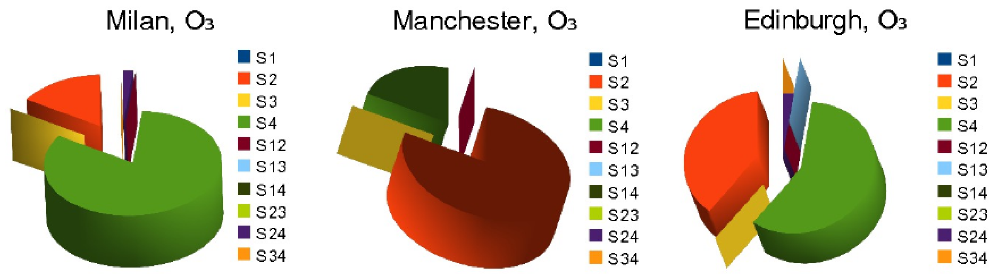
• On ozone concentrations:
  The most influential pollutant emissions in Milan and Edinburgh are anthropogenic hydrocarbons (59–83%), whereas nitrogen oxides play a dominant role (79%) in Manchester. In the areas of Milan and Edinburgh, nitrogen oxides emissions (16–39%) have a significant influence. The impact of nitrogen oxides emissions and anthropogenic hydrocarbons is relatively balanced in Edinburgh. Second-order interaction effects in Manchester are almost negligible (even $S_{24}\ll 0.1\%$), whereas in Milan and Edinburgh, the joint effect accounts for approximately 2%. Total effects are primarily driven by the corresponding main effects, but Milan and Edinburgh also exhibit a slight contribution from the joint effects of anthropogenic hydrocarbons and nitrogen oxides emissions.
• On ammonium sulfate and ammonium nitrate concentrations:
  The most influential pollutant emissions are sulfur dioxide emissions (58–82%), with ammonia emissions also having a significant but smaller impact (15–39%). In Manchester, the influence of ammonia and sulfur dioxide emissions is comparatively balanced. All four groups of pollutants have an influence on the considered important species, with nitrogen oxides and anthropogenic hydrocarbons exhibiting a slight but not negligible effect. Second-order effects in the Manchester area are mostly negligible, except for $S_{13}\approx 2.5\%$. In Edinburgh, three second-order interaction effects contribute to the corresponding total effects (0.1–3.3%).

The following observations for SIs can be made regarding the SSIEL:

• From Table 3, it can be deduced that the most effective algorithms of all of the first-order SIs and TSIs, the most accurate is the order-dependent weight lattice, except for $S_2$ and $S_2^{tot}$, where the Sobol–Burkardt algorithm produces better results.
• The product weight lattice is generally worse than the order-dependent lattice, but it produce the same relative error for $S_3$ and $S_3^{tot}$.
• In [67], it is emphasized that having the smallest possible SIs is crucial for the model. In our case, these smallest SIs are $S_4$ and $S_4^{\mathrm{tot}}$, and the order-dependent weight lattice outperform the other sequences for these SIs, but for $S_4$ the digital Sobol algorithm produced the same relative error as the order-dependent weight lattice.
• Generally, in the case of SSIEL, our lattice sequences yield significantly better results than the original Sobol sequence and its modifications, namely MCA-MSS-1, 2, and 2S.

Similarly, in the case of the SSCRR, the following can be observed:

• For a sample size of $N=2^{16}$ in Table 4, order-dependent weight lattice produces the best results for most of the cases, except $S_5$, $S_6$, $S_1^{tot}$, $S_2^{tot}$, $S_3^{tot}$, $S_6^{tot}$, and $S_{45}$.
• As mentioned earlier, having the smallest possible SIs is crucial for the model. In this case, these smallest SIs are $S_5$, $S_{45}$, and $S_5^{\mathrm{tot}}$, and the product weight lattice produce better results than the other algorithms for these SIs, only in the case of $S_5^{\mathrm{tot}}$ Sobol–Burkardt produce the same result as product weight lattice.
• The digital Sobol sequence is the most accurate for $S_6$, $S_1^{tot}$, and $S_2^{tot}$, whereas Sobol–Burkardt is the most accurate for $S_3^{tot}$.
• Generally, the order-dependent weighted and product weighted lattice significantly outperforms the original Sobol sequence and its modifications, MCA-MSS-1, -2, and -2S.

In conclusion, the two developed lattices are the most effective approaches among the benchmarked methods, as indicated by the relative error values. For some of the SIs, the most well-known Sobol algorithms, the digital Sobol and Sobol–Burkardt algorithms, produce slightly better results, but this is not the case for the smallest in value SIs. When applied to multidimensional air pollution sensitivity analysis, these sequences demonstrate superiority over the majority of existing methods. It should be noted that the lattice with a generating vector consisting of a prime number of points and with product weights produce the best results for the smallest in value SIs for the second case of SSCRR, whereas the lattice with the generating vector, a prime number of points, and order-dependent weights produces the most accurate results for the smallest in value SIs for the first case of SSIEL.

8. Conclusions

This study focuses on the application of a sophisticated digital twin named DIGITAL AIR to examine the problem of high air pollution levels in different regions of Europe. The study employs a range of tools and techniques to effectively investigate this issue.

The UNI-DEM mathematical model plays a central role in this study, requiring the implementation of highly efficient and accurate numerical algorithms. These algorithms are executed on state-of-the-art supercomputers to ensure reliable and precise simulations of air pollution dynamics.

To support the modeling efforts, extensive datasets are utilized, encompassing meteorological data, emission data, and geographical information. These datasets provide essential input parameters for the simulations and contribute to the overall accuracy and reliability of the findings.

To account for future climate changes and their impact on air pollution, the study incorporates carefully designed climatic scenarios. These scenarios consider the anticipated increase in temperatures and the corresponding changes in natural (biogenic) emissions. By incorporating these future projections, the study aims to provide insights into the potential long-term effects of climate change on air quality.

Visualizing the obtained numerical results is an integral part of the study, and graphical programs are employed for this purpose. These programs enable the researchers to analyze and interpret the simulation outcomes in a visually accessible manner, facilitating a comprehensive understanding of the complex air pollution patterns.

Additionally, this study introduces a further exploration of DIGITAL AIR through a multidimensional sensitivity analysis conducted using advanced stochastic methods based on superconvergent lattice sequences. This analysis aims to investigate the sensitivity of the model and its outputs to variations in input parameters and uncertainties. By employing stochastic techniques, the study can account for the inherent randomness and variability in the system, leading to a more comprehensive understanding of the model’s behavior and its robustness in different scenarios.

In summary, this research utilizes the DIGITAL AIR digital twin and employs a range of tools, including the UNI-DEM mathematical model, extensive datasets, carefully designed climatic scenarios, and graphical programs for visualization. The investigation is extended through a sensitivity analysis using advanced stochastic methods based on powerful lattice and digital sequences, contributing to a more comprehensive understanding of air pollution dynamics and the potential impacts of climate change.

The current version of UNI-DEM, although a powerful mathematical model for air pollution analysis, has certain limitations that should be acknowledged. One notable limitation is that it does not account for PM10 (consists of small particles suspended in the air, such as dust, pollen, soot, and other solid or liquid pollutants) in its calculations. These particles are small enough to be inhaled into the respiratory system, posing potential health risks. Monitoring and controlling PM10 levels is crucial for assessing air quality and understanding its impact on human health and the environment. However, future iterations of UNI-DEM are expected to address this limitation by incorporating PM10 data and considering their impact on air pollution dynamics. By taking into account this important particulate matter, the model will provide a more comprehensive and accurate representation of air quality, contributing to a deeper understanding of the factors influencing air pollution levels.

In future research, a more comprehensive comparison will be conducted between the newly developed lattice approach and the most advanced digital sequences. The aim will be to explore and evaluate the performance of these methods in greater detail. Moreover, the results of our study presented in this paper through sensitivity analysis will have a multifaceted and highly significant impact. By utilizing the insights gained from our sensitivity analysis, the mathematical model will provide a more precise assessment of agricultural losses. Additionally, it will serve a crucial role in estimating the detrimental effects of emissions on human health.