Article

Assimilation of FY-3D and FY-3E Hyperspectral Infrared Atmospheric Sounding Observation and Its Impact on Numerical Weather Prediction during Spring Season over the Continental United States

1
Meteomatics AG, Unterstrasse 12, 9000 St. Gallen, Switzerland
2
Space Science and Engineering Center, University of Wisconsin-Madison, Madison, WI 53706, USA
3
School of Environment, Nanjing Normal University, Nanjing 210098, China
*
Author to whom correspondence should be addressed.
Atmosphere 2023, 14(6), 967; https://doi.org/10.3390/atmos14060967
Submission received: 9 April 2023 / Revised: 27 May 2023 / Accepted: 29 May 2023 / Published: 1 June 2023
(This article belongs to the Special Issue Advances in Severe Weather Forecast)

Abstract

:
As a part of the World Meteorological Organization (WMO) Global Observing System, HIRAS-1 and HIRAS-2’s observations’ impact on improving the accuracy of numerical weather prediction (NWP) can be summarized into two questions: (1) Will HIRAS observation help the NWP system to improve its accuracy? (2) Which instrument has the greater impact on NWP? To answer the questions, four experiments are designed here: (I) the HIRAS-1 experiment, which assimilates the principal component (PC) scores derived from HIRAS-1 radiance observation from the FY-3D satellite; (II) the HIRAS-2 experiment, which assimilates HIRAS-2 (onboard the FY-3E satellite) radiance-observation-derived PC scores; (III) the J-01 experiment, which assimilates JPSS1 CrIS radiance-observation-derived PC scores; (IV) the control experiment. Each experiment generated a series of forecasts with 24 h lead-time from 16 March 2022 to 12 April 2022 using the Unified Forecast System Short-Range Weather application. Forecast evaluation using radiosonde and aircraft observation reveals: (a) for upper-level variables (i.e., temperature and specific humidity), assimilating HIRAS observation can improve the NWP’s performance by decreasing the standard deviation (Stdev) and increasing the anomaly correlation coefficient (ACC); (b) according to the multi-category Heidke skill score, HIRAS assimilation experiments, especially the HIRAS-2 experiment, have a higher agreement with hourly precipitation observations; (c) based on two tornado-outbreak case studies, which occurred on 30 March 2022 and 5 April 2022, HIRAS observation can increase the predicted intensity of 0–1 km storm relative helicity and decrease the height of the lifted condensation level at tornado outbreak locations; and (d) compared to CrIS, HIRAS-2 still has room for improvement.

1. Introduction

Observations from hyperspectral infrared sounders, e.g., the Atmospheric Infrared Sounder (AIRS), the Infrared Atmospheric Sounding Interferometer (IASI) and the Cross-track Infrared Sounder (CrIS), can improve the accuracy of numerical weather prediction (NWP) in both global and regional scales. Studies have proved that this improvement derives from the decrease of the initial condition’s systematic and random error, benefiting from the assimilation of hyperspectral infrared sounding data [1,2,3,4,5,6,7,8,9,10]. Observing simulated system experiments (OSSE) also illustrates that observations from more-advanced hyperspectral infrared sounders, e.g., IASI New Generation (IASI-NG), can be more influential if they are assimilated in NWP systems [11].
As China’s polar-orbiting meteorological satellites become an essential part of the global polar-orbiting satellite observing system, more and more observations have been adopted by various operational NWP centers. Among the payloads onboard the FY-3 series platforms, it is the microwave temperature sounding data, i.e., MWTS-1, -2, -3 and MWHS-2 that is widely used [12,13,14,15,16,17]. Recently, operational NWP centers started paying attention to the hyperspectral infrared sounding observations gathered by the Hyperspectral Infrared Atmospheric Sounder (HIRAS) onboard FY-3D [18,19]. The results reveal that most forecast variables up to a 7-day lead time can obtain improvements from HIRAS observation assimilation, with a 0.1 to 0.5% root–mean–square error (RMSE) deduction. The FY-3E satellite was successfully launched into early-morning orbit on 5 July 2021 [20]. This satellite carries a second-generation hyperspectral infrared atmospheric sounder (HIRAS-2). For the spectral coverage (Figure 1), HIRAS-2 shares the same spectral resolution (0.625 cm−1) but has a comprehensive coverage from 650 cm−1 to 2550 cm−1. As for the spatial coverage, HIRAS-2 increases its detecting-array size (nadir resolution) to 3 × 3 (14 km) but decreases the swath width (scan lines) to 2260 km (28), while HIRAS-1 has the smaller detecting array ( 2 × 2 ) and lower nadir resolution (16 km) but the larger swath (with 2400 km) and scan line amount (29); these differences can be detected in Figure A1 in Appendix A. In terms of the observation quality, Figure 2 demonstrates the Noise-equivalent differential radiance ( N E Δ R ) of HIRAS-2, which is smaller than the previous generation (HIRAS-1), especially in the mid- and short-wave infrared channel, but still larger than CrIS. A systematic evaluation study [21] also demonstrates that the performance of HIRAS-2 is more stable than HIRAS-1. The differences in instrument design raise two questions: (1) Will HIRAS observation help to improve the NWP system’s accuracy? (2) Which instrument has a higher impact on NWP, HIRAS-1 or HIRAS-2? To answer the questions, four experiments with four-week long (from 16 March 2022 to 12 April 2022, with the lack of 21 March 2022 and 22 March 2022, due to HIRAS-2 data unavailability) 24-h lead-time forecast experiments are conducted. Apart from the control experiment, in which no data assimilation process is conducted, we add another one, the CrIS experiment, to demonstrate the baseline performance of hyperspectral infrared sounding observation assimilation in the principal component space.
In the next part, Section 2 introduces the data assimilation (DA) and the NWP configurations, as well as the data used in prediction and evaluation. Section 3 presents the analysis and evaluation of the experiment’s results. The discussion and conclusion are given in Section 4 and Section 5.

2. Materials and Methods

2.1. PC-Score DA Module

In this research, we use a 3-dimensional variational (3D-Var) DA system to assimilate hyperspectral IR sounding observations in PC space. Studies have proven that the PC scores derived from hyperspectral infrared sounding observation can eliminate information redundancy, retain crucial independent information content, and improve the signal-to-noise ratio [22,23,24,25]. Specifically, principal component analysis (PCA) converts the hyperspectral infrared observations from spectrum space to “imaginary” orthometric space—principal component scores, using pre-calculated empirical orthogonal functions (EOFS). The pre-calculated EOFS is equivalent to the coefficients in channel-based radiative transfer models, e.g., the community radiative transfer model (CRTM) and the radiative transfer for TOVS (RTTOV). This process can retain crucial independent information content, decrease information redundancy and improve observation’s signal-to-noise ratio. NWP studies [26,27,28,29] have illuminated that the assimilation of PC scores can improve the initial condition’s quality and reserve computational resources. The cost function of the 3D-Var DA system is listed below:
J ( x ) = ( x x b ) T B 1 ( x x b ) + ( y H ( x ) ) T R 1 ( y H ( x ) )
In Equation (1), x ( x b ) is the analysis field (first guess field); B is the background error covariance generated from a three-month-long (from 1 January 2022 to 31 March 2022, available at https://noaa-gfs-bdp-pds.s3.amazonaws.com/index.html, accessed on 12 February 2023) NOAA Global Forecast System (GFS) forecast product using the NMC method [30]; y is the PC score derived from HIRAS-1, HIRAS-2, and J01 CrIS observations via QR decomposition, noting that the HIRAS-1 and HIRAS-2 observation can be downloaded from the National Meteorological Satellite Center’s (NSMC) Fengyun Satellite Data Center (available at http://satellite.nsmc.org.cn/PortalSite/Data/DataView.aspx, accessed on 12 February 2023), the CrIS observation is available at the NOAA Comprehensive Large Array‘s Data Stewardship System (https://www.avl.class.noaa.gov/saa/products/welcome, accessed on 12 February 2023); H is the PC-based Havemann–Taylor Fast Radiative Transfer Code (HTFRTC) [31,32]; R is the observational error covariance matrix generated from the Hollingsworth–Lönnberg method [33,34]. To conserve computational resources, the y H ( x ) is linearized to y H ( x b ) H ( x b ) · ( x x b ) , where H is the Jacobian of H and the L-BFGS-B method is selected as the cost function’s minimization method. The coefficients for HIRAS-1 and HIRAS-2 instrument are crucial to the DA system’s performance. In this research, their coefficients are generated from the ECMWF-MACC 60-Level profile dataset (https://nwp-saf.eumetsat.int/site/software/atmospheric-profile-data/, accessed on 12 February 2023) using the standard coefficient generation approach for HTFRTC [35]. For profile selection, 200 profiles from each of the temperature, water vapor, ozone, CO2, and methane dataset are randomly selected, which composes a 1000-profile training set (Figure 3).
The HTFRTC is capable of calculating as many as 300 PCs for each instrument from a certain atmospheric profile. However, it is the first 30 PCs that have a relatively high impact on the meteorological fields [36,37,38]. Given this, we only calculate the observational error covariance (R matrix) for the first 30 PCs in this research (Figure 4). If we compare the observational error covariance between HIRAS-1 (Figure 4a) and HIRAS-2 (Figure 4b), it is clear that the off-diagonal values of HIRAS-2’s R matrix are smaller than those from HIRAS-1, especially in the first 15 PCs. This indicates that HIRAS-2 retrieves more accurate observations than HIRAS-1 due to the decrease of N E Δ R , but still has notable departure if compared to CrIS (Figure 4c). In most cases, off-diagonal values in the observational error covariance are assumed to be zero in data assimilation systems and the diagonal values have the highest significance in utilizing observations, which is to say, decreasing the off-diagonal value in observational error covariance can improve the agreement between operational practice and theoretical assumption. The correlation coefficient matrices (Figure 4b,d,f) share the same conclusion as observational error covariance matrices; additionally, they also indicate that the cross-channel correlation issue can be alleviated in PC score assimilation. This is most obvious in CrIS (Figure 4f) and can be detected in HIRAS-2 (Figure 4d) and HIRAS-1 (Figure 4b) as well.
Before converting the radiance observation to PC scores, cloud screening and quality control have to be conducted to ensure (1) that the observations are from a clear-sky region and (2) the quality of each observation. In cloud detection, the clear-sky percentage in each field of view (FOV) is determined by the Advanced Baseline Imager (ABI) Full Disk Clear Sky Mask from GOES-16 (https://noaa-goes16.s3.amazonaws.com/index.html#ABI-L2-ACMF/, accessed on 12 February 2023) [39]; if the ABI clear-sky pixel amount within a HIRAS-1 (HIRAS-2 or CrIS) FOV is less than 80% of the total ABI pixel amount in the same FOV, then this FOV’s radiance observation will be discarded. After screening out the cloudy observations, the quality control process opts out the disqualified clear-sky observation using a method described as follows: the quality control converts clear-sky radiance observation to PC scores and calculates the first 30 PC scores’ mean bias ( M B ) and standard deviation ( S D ) with reference to the simulated PC scores from first guess, and if more than 25 PC scores from an observation are located within M B ± 1.5 S D then all 30 PC scores will be assimilated by the DA system.

2.2. NWP Module

The NWP module is built upon the Unified Forecast System Short-Range Weather (UFS-SRW) application version 1.0.0, which was first released in March 2021 [40]. The application includes a pre-processing utility, the FV3 Limited Area Model (LAM) [41], the Common Community Physics Package (CCPP) [42], and the Unified Post Processor (UPP). Already been chosen as the forecast module for NOAA’s next-generation Rapid Refresh Forecast System (RRFS), performance evaluation studies have revealed its functionality and accuracy [43,44]. In this research, we inherit a pre-defined 13 km horizontal domain (RRFS_CONUS_13 km, Figure 5) from UFS-SRW default domain settings which cover the continental United States (CONUS). The RRFS_v1alpha physics suite (Table 1) was adopted for all experiments.

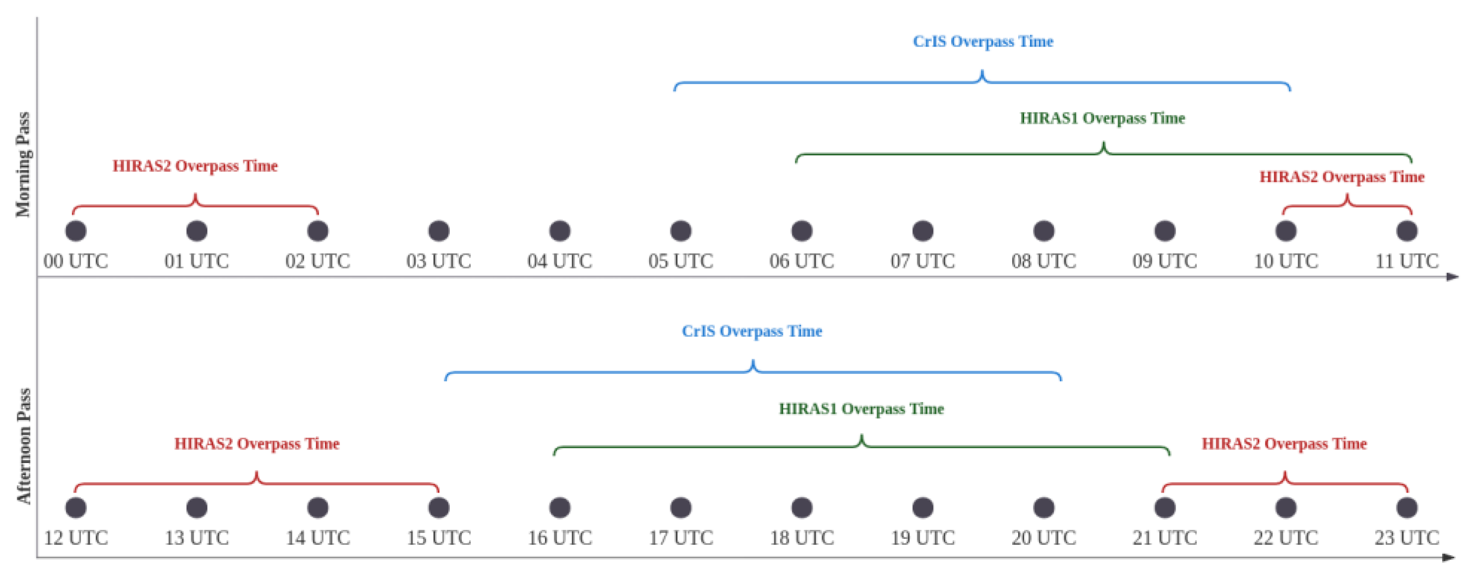
2.3. Experiment Schemata

As can be seen in Figure 6, the research consists of the three assimilation experiments which were designed, namely, the HIRAS-1, HIRAS-2, and CrIS, and each experiment only assimilates the corresponding PC scores derived from radiance observations from each of those three instruments. This can guarantee that the performance differences in the evaluation are strictly coming from the hyperspectral infrared sounding observations and ensure the evaluation results are independent.
The initial condition for the first analysis cycle and the boundary condition for the analysis and forecast cycles are provided by the NOAA GFS operational analysis product. The system started the first analysis cycle at 00:00 UTC every day from 15 March 2022 to 11 April 2022 (cold start), and the initial condition for the forecast cycle (final analysis) was generated from hourly-basis continuous analysis cycles (24 cycles in total). It is important to understand that not all analysis cycles have the observation assimilated due to the polar-orbiting satellite platform’s revisiting time vacancy. For the analysis cycles that do not have available observations to assimilate, the 1-h lead-time forecast will be conducted without initiating the DA process. After retrieving the final analysis, the forecast cycle will start generating a 24-h lead-time forecast. All three experiments share the same background error covariance. The workflow settings for the control experiment are not mentioned here, because this experiment is a dynamical down-scaling of GFS forecast product from 0.25° to 13 km horizontal resolution.

3. Results

The following part consists of four sections: Section 3.1 focuses on initial condition evaluation; Section 3.2 focuses on upper-level atmospheric variable evaluation in the forecast product; Section 3.3 focuses on hourly precipitation forecast evaluation; Section 3.4 focuses on tornado-outbreak prediction accuracy evaluation. For Section 3.1, Section 3.2 and Section 3.3, the evaluation results derive from the 24-h lead-time forecast from 15 March 2022 to 12 April 2022 (missing forecast results on 22 March and 23 March, due to HIRAS-2 observation availability). Results shown in Section 3.4 come from selected case studies, and case selection reasons will be mentioned in that section.

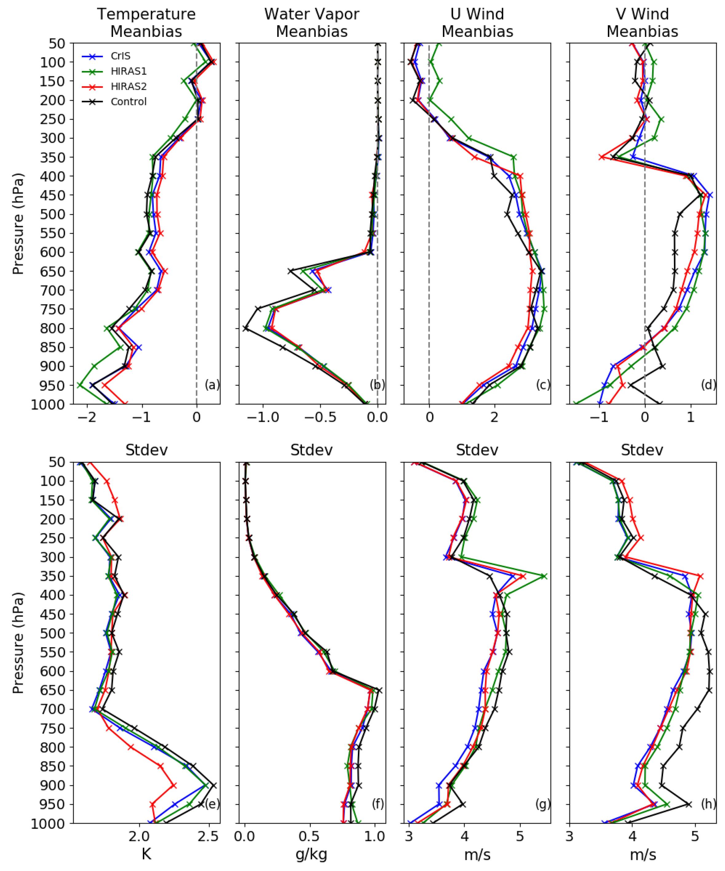
3.1. Initial Condition Performance Comparison

In this section, the initial conditions used for the 24-h predictions are evaluated against radiosonde and aircraft observations from the NCEP ADP Global Upper Air and Surface Weather Observation dataset (available at https://rda.ucar.edu/datasets/ds337-0/, accessed on 18 Feburary 2023). From the temperature mean bias profile (Figure 7a), we can find that the DA (HIRAS-1, HIRAS-2, and CrIS) experiments have better temperature field than the control experiment (GFS operational analysis field) below 850 hPa and between 700 hPa and 250 hPa, while the downscaling of GFS operational analysis is better between 750 and 850 hPa. The differences between DA experiments and GFS operational analysis are negligible above 250 hPa. As for the differences among DA experiments, the HIRAS-2 experiment has the best performance below 750 hPa, with CrIS as second-best. Between 700 and 250 hPa, CrIS experiment’s initial condition outperformed the HIRAS-1 and HIRAS-2 experiments. In terms of the water vapor mixing ratio’s mean bias (Figure 7b), the DA experiments are slightly better than the GFS operational analysis at the near-surface layer, but a higher departure between 950 and 650 hPa was observed. Compared with the CrIS experiment, the HIRAS-2 experiment has a slightly larger departure below 950 hPa, but its accuracy is much better than CrIS between 950 and 600 hPa. The HIRAS-1’s accuracy is comparable to HIRAS-2 below 950 hPa, but decreases rapidly to becoming the worst from 950 to 600 hPa. In Figure 7c, the standard deviation of the GFS operational analysis is lower than DA experiments below 700 hPa. In addition, the HIRAS-2 experiment is better than CrIS experiment from 950 to 700 hPa. The HIRAS-1 experiment has the second-best performance between 950 and 900 hPa and smallest standard deviation at 1000 hPa, while the CrIS experiment has the second-smallest value at this level, with the HIRAS-2 as the largest. Just as with the temperature standard deviation profile, the GFS operational analysis generally has the smallest water vapor mixing ratio standard deviation (Figure 7d) among all layers, except 800 hPa. Meanwhile, the HIRAS-2 and CrIS experiments share the same accuracy below 900 hPa and from 650 to 500 hPa. Between 900 and 750 hPa, the HIRAS-2 experiment’s accuracy is relatively worse than the CrIS and HIRAS-1 experiments but has the smallest standard deviation among DA experiments at 700 hPa. From Figure 7, we can detect that the temperature field in the GFS initial condition is colder than in the observation, which can be partly corrected by hyperspectral infrared sounding assimilation; however, the added information content fails to decrease the random error (standard deviation) in the lower troposphere (below 750 hPa), because the hyperspectral infrared sounders are more sensitive to atmospheric changes above 800 hPa. Additionally, assimilating hyperspectral infrared sounding observation enlarges the embedded dry bias in GFS initial condition from 950 hPa to 650 hPa, and decreases the same value at 1000 hPa, while the standard deviation seldom changes after the assimilation process.
No significant improvement can be found in the initial conditions of all three DA experiments, as compared to the GFS operational analysis, since the GFS operational analysis assimilates many more observations, including the radiosonde and aircraft observations used for evaluation in this section. However, accuracy differences between the DA experiments are clearly revealed; in general, the HIRAS-2 experiment has the highest accuracy, followed by the CrIS and HIRAS-1 experiments. Such results can be attributed to two facts: (1) the initial condition comparisons are valid at 00:00 UTC, which agrees better with the local overpass time (Figure 8) of FY-3E’s (HIRAS-2 experiment) early-morning orbit than JPSS1 (CrIS experiment) and FY-3D (HIRAS-1 experiment); (2) the observation quality from FY-3D’s HIRAS instrument is not as good as that from FY-3E’s and is even worse than that of JPSS1 CrIS (Figure 2). In conclusion, the accuracy improvement in the HIRAS-2 experiment results from observation quality improvement and better orbit selection. To summarize, the performance fall-behind in the HIRAS-1 experiment mostly results from its inferior observation quality, since FY-3D shares almost the same local overpass time with JPSS1. However, the performance improvement in the HIRAS-2 experiment may have come about in a couple of different ways: (1) FY-3E operates in early-morning orbit, which means that the HIRAS-2 experiment can assimilate the closest-to-forecast-initialization-time observation, while the other experiments cannot; (2) HIRAS-2’s N E Δ R is smaller than HIRAS-1 and has a more comprehensive spectral coverage over the thermal infrared region.

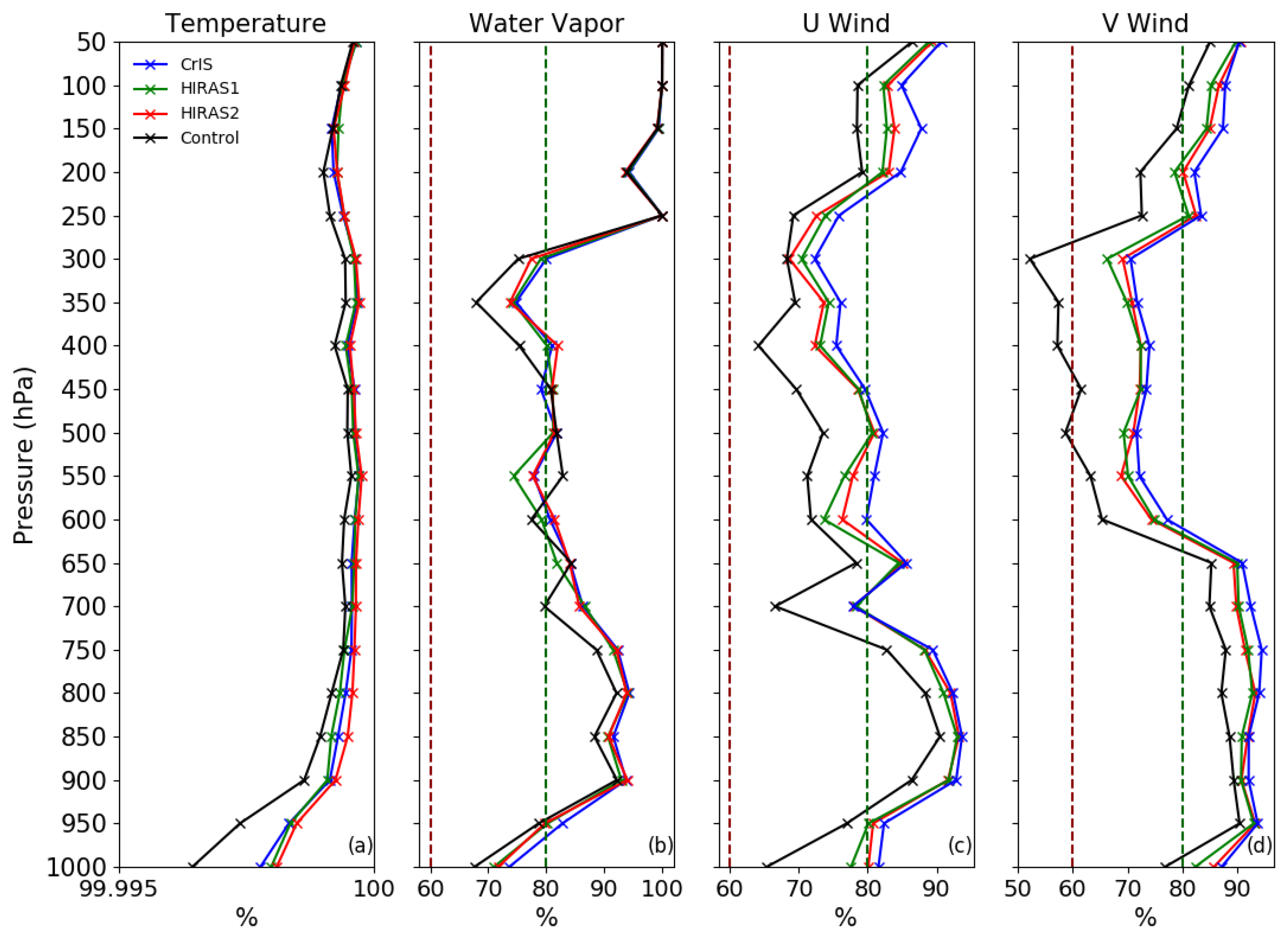
3.2. NWP Forecast Performance Comparison

The mean bias profiles of predictions at all forecast lead times are plotted in Figure 9. As shown in Figure 9a, the HIRAS-1 experiment performs worse than the control experiment below 800 hPa (above 350 hPa) but has as close a systemic error as the control between 800 and 350 hPa. Unlike the HIRAS-1 experiment, the absolute values of mean bias from CrIS and HIRAS-2 experiments are generally smaller than the control experiment. The mean bias profiles of the water vapor mixing ratio (Figure 9b) indicate that all DA experiments are constantly better than the control, but performance differences between DA experiments still exist: a larger bias is found between 700 and 650 hPa from the HIRAS-1 experiment compared to the other DA experiments. The zonal wind (U wind) mean bias profiles (Figure 9c) show that the HIRAS-2 experiment has the best performance below 600 hPa, while the control experiment has the best performance between 600 and 350 hPa. The CrIS experiment’s U-wind accuracy stays between the HIRAS-2 and the control experiment. The HIRAS-2, CrIS, and control experiments have similar performance at levels above 350 hPa. The HIRAS-1 experiment’s performance is generally worse than the control experiment above 750 hPa, but it has equivalent performance below 800 hPa. All experiments tend to overestimate the meridional wind (V wind) speed between 850 and 350 hPa, and underestimations of V wind below 900 hPa (Figure 9d) are observed in the DA experiments. In general, the HIRAS-2 experiment has higher accuracy in meridional wind prediction than do the CrIS and HIRAS-1 experiments. The temperature standard deviation profile in Figure 9e demonstrates that assimilating hyperspectral infrared sounding observations can reduce the random error in the NWP product, since the standard deviations of DA experiments are smaller than that of the control experiment. In addition, we can find that HIRAS-2 observation is better at reducing NWP temperature random error below 700 hPa than CrIS and HIRAS-1 observations but the advantage disappears at and above 650 hPa. The HIRAS-1 observation can decrease the random error, but with a smaller reduction magnitude compared to the CrIS experiment. The results from the water-vapor mixing-ratio standard deviation profiles (Figure 9f) are basically similar to temperature standard deviation: (1) evaluations (except the HIRAS-1 experiment’s result at 1000 hPa) show that assimilating hyperspectral infrared sounding observation can reduce the random error in the NWP water vapor product; (2) the HIRAS-2 experiment shares a similar performance, with the CrIS experiment and the random error reduction capability in HIRAS-1 experiment smaller than in the other two DA experiments. In wind prediction (Figure 9g,h), the CrIS experiment has the smallest standard deviation, and DA experiments are better than the control experiment below 400 hPa, and worse above 300 hPa. Performance degradation can be detected in the HIRAS-1 and HIRAS-2 experiments, but the HIRAS-2 experiment still possesses performance enhancement over the HIRAS-1 experiment. It is interesting that the vertical performance vibration from 1000 hPa to 950 hPa exists in wind evaluation, especially the v-component wind (Figure 9h). This is mainly due to the level of the vertical distribution of aircraft observation: according to the report from World Meteorological Organization (WMO) [45], the aircraft observation amount at near-surface (1000 ± 25 hPa) is extremely small, and the observation amount starts climbing up during the landing and taking-off processes. Generally, the first available observation’s pressure level is located between 975 hPa and 925 hPa. The vertical distribution inequality of aircraft observation also contributes to the specific humidity’s similar performance at the upper atmosphere: aircraft generally observes the temperature and wind over the upper troposphere while water vapor observations are gathered over middle and low troposphere. Due to the relatively homogeneous observation amounts in vertical scale, the problem listed above is less detectable in temperature evaluation.
The uncentered anomaly correlation coefficient ( A C C , Equation (2)) [46] profiles derived from the 1–24 h lead-time forecast in Figure 10 can reveal the impact differences from HIRAS-1, HIRAS-2, and CrIS observations on NWP in a clearer view. In Equation (2), F stands for the forecast variables (i.e., temperature, water vapor, u-wind, and v-wind); C stands for the climatological mean; in this case, it is calculated from 2003 to 2022 using the ECMWF Reanalysis v5 (ERA5, available at https://cds.climate.copernicus.eu/cdsapp#!/dataset/reanalysis-era5-pressure-levels?tab=form, accessed on 18 February 2023); and O stands for radiosonde and aircraft observation. Typically, a forecast performance is “good” (“fair”) if the A C C is higher than 80% (between 60% and 80%) [47]. In temperature prediction (Figure 10a), the DA experiments performed better than the control experiment. The HIRAS-2 experiment performed slightly better than the CrIS and the HIRAS-1 experiments and the advantage in the CrIS experiment was marginal compared to the HIRAS-1 experiment. From the water vapor mixing ratio’s A C C profile (Figure 10b), we can tell that (1) all experiments have a “fair” performance of predicting near surface and 450–300 hPa water vapor but the performance is “good” at other levels; (2) the DA experiments acquire better performance than that of the control experiment, and the CrIS experiment is the best; and (3) the HIRAS-1 and HIRAS-2 experiments’ performance is identical except at levels between 700 and 500 hPa. In wind prediction (Figure 10c,d), DA experiments precede the control experiment to a relatively higher degree, compared to temperature and water vapor. In the same manner as the result from the water-vapor mixing ratio, the CrIS experiment has the best performance in predicting zonal and meridional wind, and the HIRAS-2 experiment performs better than the HIRAS-1 experiment but with narrow A C C value margins.
A C C = ( F C ) ( O C ) ( F C ) 2 ( O C ) 2

3.3. Hourly Quantitative Precipitation Forecast (QPF) Evaluation

In this section, each experiment’s 3–24 h lead-time QPF accuracy is represented by a multi-category Heidke skill score ( H S S , Equation (3)) [48], where n ( F i , O i ) is the number of grids where forecasts and observations are located within the same criteria i , N ( F i ) represents the number of grids where forecasts are within criteria i , and N(Oi) is the number of grids where observations are within criteria i . To calculate the score, forecasts and observations are scaled to three categories using the thresholds in Table 2. In this case, the observations come from the NCEP/EMC 4 km gridded multi-sensor hourly precipitation dataset (available at https://data.eol.ucar.edu/dataset/21.093, accessed on 16 Feburary 2023); this product is spatially downscaled to 13 km resolution via a nearest-9–gridpoint average interpolation method to decrease the representative error between forecast and observation. From each DA experiment’s H S S departure from the control experiment in Figure 11, we can conclude that the hyperspectral infrared sounding observation from HIRAS-1, HIRAS-2, and CrIS can improve the NWP system’s QPF accuracy. Due to local overpass time and observation quality, HIRAS-1 contributes the smallest performance improvement. Compared to the CrIS experiment, accuracy improvement from HIRAS-2 observation assimilation is slightly smaller at the first 10 forecasts’ lead-time, but higher after the 11th forecast’s lead-time. This symptom could result from the dynamical—microphysics balance adjustment inside UFS-SRW: as can be seen in Figure 8, the last analysis cycle with DA capability enabled typically ended before 21:00 UTC in the CrIS experiment; this offers the forecast cycle extra time to finish the balance adjustment, while the HIRAS-2 experiment still initializes the DA process in its forecast cycle (at 00:00 UTC). The HIRAS-1 experiment’s performance surprisingly precedes CrIS and HIRAS-2 experiments between 18 h and 21 h forecast lead-time; the cause of this issue still needs further investigation. The false alarm rate (Figure A2a) and probability of detection (Figure A2b) results share the same conclusion as the HSS evaluation, which can be found in Appendix A.
H S S = 1 N i = 1 k n ( F i , O i ) 1 N 2 i = 1 k N ( F i ) N ( O i ) 1 1 N 2 i = 1 k N ( F i ) N ( O i )

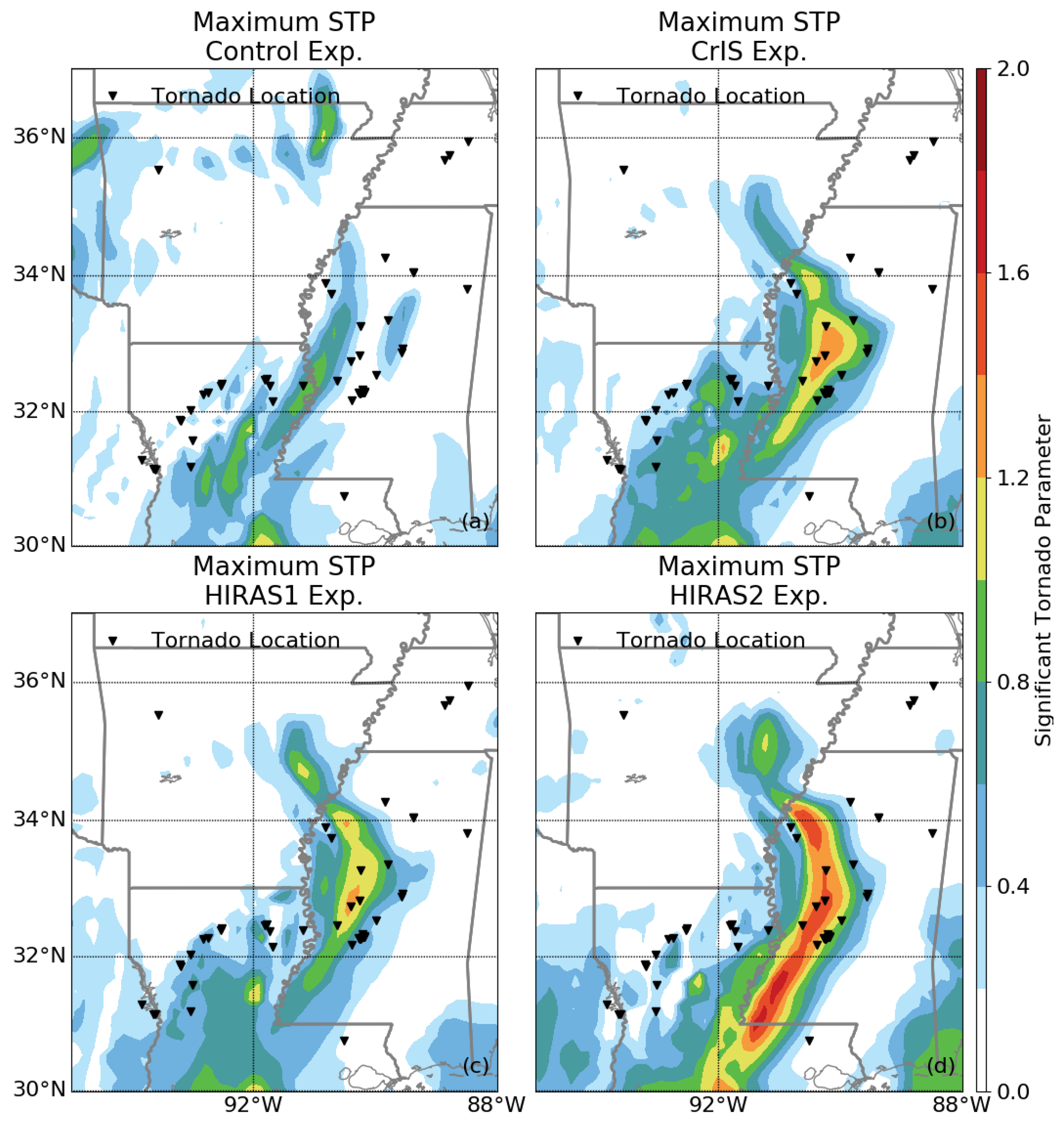
3.4. Tornado Outbreak Prediction Performance Comparison—Case Studies

Twelve tornado outbreak cases took place from 16 March 2022 to 12 April 2022. Three of them caused more than one death and four of them caused more than 50 tornado occurrence records (Table 3). Due to the HIRAS-2’s observation unavailability on 21 and 22 March 2022, two cases (30 March 2022 and 5 April 2022) are included in this section.

3.4.1. 30 March 2022 Case

Figure 12 displays the maximum significant tornado parameter ( S T P , Equation (4)) [49] from each experiment’s forecast between 13:00 UTC 30 March 2022 and 00:00 UTC 31 March 2022, where M U C A P E represents the most-unstable convective available potential energy; S R H 1 k m stands for the surface-to-1-km altitude ground-level storm relative helicity; B W D 6 k m stands for the surface-to-6-km altitude ground-level bulk wind shear; L C L stands for the Lifted Condensation Level and M U C I N stands for the Most-Unstable Convective INhibition. A total of 48 tornadoes took place during this time. In the control experiment, S T P values at 25 tornadoes’ outbreak locations were smaller than 0.2 ( m i s s ). This amount goes down to 11 in the CrIS experiment and becomes slightly smaller (10) in the HIRAS-1 and HIRAS-2 experiments. According to the miss-alarm ratio ( m i s s / t o t a l ), observation from CrIS, HIRAS-1, HIRAS-2 instruments share almost the same capability of improving NWP system’s accuracy. However, from the aspect of diagnostic variable intensity, it is clear that the S T P maximum intensity values from the CrIS and HIRAS-2 experiments are higher than the HIRAS-1 experiment and that the HIRAS-2 experiment has the highest value. This indicates that the experiments that assimilated HIRAS-2 and CrIS observations produced a more favorable tornado-genesis environment. If we compare the variables consisting of S T P (Figure 13), which are M U C A P E , scaled by 100 J/kg, Lifted Condensation Level ( L C L , scaled by 100 m), S R H 1 k m , scaled by 10 m2/s2, B W D 6 k m , scaled by 20 m/s, M U C I N , scaled by 10 J/kg, the cause of S T P increase in DA experiments is intuitive: the assimilation of hyperspectral infrared sounding observations increase (decrease) the magnitude of M U C A P E , S R H 1 k m , B W D 6 k m ( M U C I N , L C L ). Among all variables, the SRH1km and L C L has more detectable change than the other variables.
S T P = M U C A P E 1500 J / k g · 2000 m L C L 1000 m · S R H 1 k m 150 m 2 / s 2 · B W D 6 k m 20 m / s · 200 J / k g + M U C I N 150 J / k g

3.4.2. 5 April 2022 Case

Figure 14 shows the maximum S T P from each experiment’s forecast between 12:00 UTC 5 April 2022 and 00:00 UTC 6 April 2022; 55 tornadoes took place during this time. In the control experiment, S T P values at 20 tornadoes’ outbreak locations were smaller than 0.2. With 23 tornadoes’ outbreak location’s S T P value under 0.2, HIRAS-1 observation’s impact on NWP system’s performance is controversial. In contrast, the miss-alarm ratio in HIRAS-2 experiment still decreased marginally, which implies that the HIRAS-2 observation still has a potential to improve the NWP system’s high-impact weather prediction accuracy. Among the DA experiments, observation from CrIS instrument showed a great potential for increasing the NWP system’s forecast accuracy as to tornado outbreaks: there are only five tornadoes whose S T P is smaller than 0.2. The reason for HIRAS-1 and HIRAS-2 experiments’ performance discrepancy can be found in Figure 15: HIRAS-1 and HIRAS-2 experiments’ M U C A P E and B W D 6 k m ( S R H 1 k m ) magnitude are comparable to (smaller than) the CrIS experiment, but the M U C I N and L C L are larger. Regardless of the differences in the 30 March 2022 and 5 April 2022 cases, they do have one conclusion in common, which can be found in Figure 13 and Figure 15: The assimilation of hyperspectral infrared sounding observation increases the magnitude of S R H 1 k m in the NWP product.

4. Discussion

Evaluation results from Section 3 revealed that hyperspectral infrared sounding observation, including, but not limited to, HIRAS-1, HIRAS-2, and CrIS, can (1) improve regional short-range weather predictions’ accuracy as to temperature, water-vapor mixing ratio, and wind forecast in the troposphere; (2) decrease the 3–24 h lead-time forecast hourly precipitation bias; (3) minimize the miss-alarm ratio in high-impact weather outbreak prediction, e.g., tornadoes, by producing an environment that favors the generation of tornadoes. However, instrument-related performance differences can’t be neglected: the HIRAS-2 experiment’s performance is generally better than that of the HIRAS-1 experiment due to the broader spectral coverage, and higher observation quality (low N E Δ R ), as well as a higher spatial resolution; compared to CrIS, HIRAS-2’s performance still has room for improvement.
The conclusions also bring us a few unsolved questions. For example: (1) Does the relatively equivalent performance between the HIRAS-2 and CrIS experiments imply that the relatively low observation quality can be compensated for by a well-selected orbit overpass time and a higher spectrum amount? (2) Which parameter(s) is(are) dominating the performance differences in the HIRAS-1 and HIRAS-2 experiments; is it the spectral resolution or the observation quality? To answer these questions, further investigations are needed.

5. Conclusions

In this research, we set up a DA–NWP system which was capable of assimilating the PC scores derived from hyperspectral infrared sounding observations and generating a 24-h lead-time forecast dataset which contained three DA (HIRAS-1, HIRAS-2, and CrIS), and one control experiment to investigate the HIRAS observations’ impact on the accuracy improvement of numerical weather prediction, as well as demonstrating the performance differences between HIRAS-1 and HIRAS-2 observation. The research reveals: (1) both HIRAS-1 and HIRAS-2 can improve the NWP system’s forecast accuracy, and HIRAS-2 contributes more impact on NWP accuracy than HIRAS-1; (2) compared to CrIS onboard JPSS1, HIRAS-2’s performance is generally comparable and better as to temperature and 11–23 h lead-time forecast. The performance improvement can be attributed to HIRAS-2’s new spectrum design and improved observation quality ( N E Δ R decrease), as well as the FY-3E satellite’s early-morning orbit. Although positive impact on NWP can be detected when HIRAS-2 observation is assimilated, the limitations are negligible: (1) the experiments were conducted at a short-range lead-time and regional scale; more experiments at different lead-time range, different region, or global scale are still needed; (2) the experiments lasted for roughly one month, which could be treated as an extended-range case study; the conclusions demonstrated in this article may be less valid under different scenarios; additional studies in different seasons (e.g., summer) and different atmospheric situations (e.g., hurricanes) are still needed.

Author Contributions

Conceptualization, Q.Z.; methodology, Q.Z.; software, Q.Z.; validation, Q.Z.; resources, M.S.; writing—original draft preparation, Q.Z.; writing—review and editing, M.S.; funding acquisition, M.S. All authors have read and agreed to the published version of the manuscript.

Funding

The research is funded by Special Science and Technology Innovation Program for Carbon Peak and Carbon Neutralization of Jiangsu Province (Grant Number BE2022612).

Institutional Review Board Statement

Not applicable.

Informed Consent Statement

Not applicable.

Data Availability Statement

The online access URLs are provided at the first location where the data are mentioned in the article.

Acknowledgments

We thank the editors for their academic editing services. We would also like to show our gratitude to all “anonymous” reviewers for their insights and comments on an earlier version of the manuscript, although any errors are our own and should not tarnish the reputations of these esteemed persons.

Conflicts of Interest

The authors declare no conflict of interest.

Appendix A

Figure A1. The spatial resolution difference between HIRAS2 (a) and HIRAS1 (b).
Atmosphere 14 00967 g0a1
Figure A2. HIRAS-1 (green), HIRAS-2 (red) and CrIS (blue) experiments’ 3–24 h lead time probability of detection (a) and false alarm rate (b) departure from control experiment, for precipitation intensity higher than 1 mm/h.
Atmosphere 14 00967 g0a2

References

  1. Fourri’e, N.; Thépaut, J.N. Evaluation of the AIRS near-real-time channel selection for application to numerical weather prediction. Q. J. R. Meteorol. Soc. 2003, 129, 2425–2439. [Google Scholar] [CrossRef]
  2. Gambacorta, A.; Barnet, C.D. Methodology and information content of the NOAA NESDIS operational channel selection for the Cross-Track Infrared Sounder (CrIS). IEEE Trans. Geosci. Remote Sens. 2012, 51, 3207–3216. [Google Scholar] [CrossRef]
  3. Collard, A.D. Selection of IASI channels for use in numerical weather prediction. Q. J. R. Meteorol. Soc. 2007, 133, 1977–1991. [Google Scholar] [CrossRef]
  4. Collard, A.D.; McNally, A.P. The assimilation of infrared atmospheric sounding interferometer radiances at ECMWF. Q. J. R. Meteorol. Soc. 2009, 135, 1044–1058. [Google Scholar] [CrossRef]
  5. Coopmann, O.; Guidard, V.; Fourrié, N.; Josse, B.; Marécal, V. Update of Infrared Atmospheric Sounding Interferometer (IASI) channel selection with correlated observation errors for numerical weather prediction (NWP). Atmos. Meas. Tech. 2020, 13, 2659–2680. [Google Scholar] [CrossRef]
  6. Noh, Y.C.; Sohn, B.J.; Kim, Y.; Joo, S.; Bell, W.; Saunders, R. A new Infrared Atmospheric Sounding Interferometer channel selection and assessment of its impact on Met Office NWP forecasts. Adv. Atmos. Sci. 2017, 34, 1265–1281. [Google Scholar] [CrossRef]
  7. Hilton, F.; Atkinson, N.C.; English, S.J.; Eyre, J.R. Assimilation of IASI at the Met Office and assessment of its impact through observing system experiments. Q. J. R. Meteorol. Soc. 2009, 135, 495–505. [Google Scholar] [CrossRef]
  8. Geer, A.J.; Lonitz, K.; Weston, P.; Kazumori, M.; Okamoto, K.; Zhu, Y.; Schraff, C. All-sky satellite data assimilation at operational weather forecasting centres. Q. J. R. Meteorol. Soc. 2018, 144, 1191–1217. [Google Scholar] [CrossRef]
  9. Noh, Y.C.; Huang, H.L.; Goldberg, M.D. Refinement of CrIS channel selection for global data assimilation and its impact on the global weather forecast. Weather. Forecast. 2021, 36, 1405–1429. [Google Scholar] [CrossRef]
  10. Li, X.; Zou, X. Bias characterization of CrIS radiances at 399 selected channels with respect to NWP model simulations. Atmos. Res. 2017, 196, 164–181. [Google Scholar] [CrossRef]
  11. Andrey-Andrés, J.; Fourrié, N.; Guidard, V.; Armante, R.; Brunel, P.; Crevoisier, C.; Tournier, B. A simulated observation database to assess the impact of the IASI-NG hyperspectral infrared sounder. Atmos. Meas. Tech. 2018, 11, 803–818. [Google Scholar] [CrossRef]
  12. Lu, Q.; Bell, W.; Bormann, N.; Bauer, P.; Peubey, C.; Geer, A.J. Improved assimilation of data from China’s FY-3A microwave temperature sounder. Atmos. Sci. Lett. 2012, 13, 9–15. [Google Scholar] [CrossRef]
  13. Carminati, F.; Migliorini, S. All-sky data assimilation of MWTS-2 and MWHS-2 in the Met Office global NWP system. Adv. Atmos. Sci. 2021, 38, 1682–1694. [Google Scholar] [CrossRef]
  14. Li, J.; Liu, G. Direct assimilation of Chinese FY-3C Microwave Temperature Sounder-2 radiances in the global GRAPES system Atmos. Meas. Tech. 2016, 9, 3095–3113. [Google Scholar] [CrossRef]
  15. Li, J.; Qian, X.; Qin, Z.; Liu, G. Direct Assimilation of Chinese FY-3E Microwave Temperature Sounder-3 Radiances in the CMA-GFS: An Initial Study. Remote Sens. 2022, 14, 5943. [Google Scholar] [CrossRef]
  16. Niu, Z.; Zou, X.; Huang, W. Typhoon Warm-Core Structures Derived from FY-3D MWTS-2 Observations. Remote Sens. 2021, 13, 3730. [Google Scholar] [CrossRef]
  17. Song, L.; Shen, F.; Shao, C.; Shu, A.; Zhu, L. Impacts of 3DEnVar-Based FY-3D MWHS-2 Radiance Assimilation on Numerical Simulations of L and falling Typhoon Ampil (2018). Remote Sens. 2022, 14, 6037. [Google Scholar] [CrossRef]
  18. Carminati, F. A channel selection for the assimilation of CrIS and HIRAS instruments at full spectral resolution. Q. J. R. Meteorol. Soc. 2022, 148, 1092–1112. [Google Scholar] [CrossRef]
  19. Qi, C.; Wu, C.; Hu, X.; Xu, H.; Lee, L.; Zhou, F.; Zhang, P.; Gu, M.; Yang, T.; Shao, C.; et al. High spectral infrared atmospheric sounder (HIRAS): System overview and on-orbit performance assessment. IEEE Trans. Geosci. Remote Sens. 2020, 58, 4335–4352. [Google Scholar] [CrossRef]
  20. Zhang, P.; Hu, X.; Lu, Q.; Zhu, A.; Lin, M.; Sun, L.; Chen, L.; Xu, N. FY-3E: The First Operational Meteorological Satellite Mission in an Early Morning. Orbit Adv. Atmos. Sci. 2022, 39, 1–8. [Google Scholar] [CrossRef]
  21. Chen, H.; Guan, L. Assessing FY-3E HIRAS-II Radiance Accuracy Using AHI and MERSI-LL. Remote Sens. 2022, 14, 4309. [Google Scholar] [CrossRef]
  22. Huang, H.; Antonelli, P. Application of principal component analysis to high-resolution infrared measurement compression and retrieval. J. App. Meteorol. 2001, 40, 365–388. [Google Scholar] [CrossRef]
  23. Antonelli, P.; Revercomb, H.E.; Sromovsky, L.A.; Smith, W.L.; Knuteson, R.O.; Tobin, D.C.; Garcia, R.K.; Howell, H.B.; Huang, H.; Best, F.A. A principal component noise filter for high spectral resolution infrared measurements. J. Geophys. Res. 2004, 109, D23102. [Google Scholar] [CrossRef]
  24. Goldberg, M.D.; Zhou, L.; Wolf, W.W.; Barnet, C.; Divakarla, M.G. Applications of principal component analysis (PCA) on AIRS data. In Proceedings of the Multispectral and Hyperspectral Remote Sensing Instruments and Applications II, Honolulu, HI, USA, 9–11 November 2004. [Google Scholar] [CrossRef]
  25. Tobin, D.C.; Antonelli, P.B.; Revercomb, H.E.; Dutcher, S.T.; Turner, D.D.; Taylor, J.K.; Vinson, K.H. Hyperspectral data noise characterization using principal component analysis: Application to the atmospheric infrared sounder. J. Appl. Remote Sens. 2005, 1, 013515. [Google Scholar] [CrossRef]
  26. Matricardi, M.; McNally, A.P. The direct assimilation of principal components of IASI spectra in the ECMWF 4D-Var. Q. J. R. Meteorol. Soc. 2014, 140, 573–582. [Google Scholar] [CrossRef]
  27. Collard, A.D.; McNally, A.P.; Hilton, F.I.; Healy, S.B.; Atkinson, N.C. The use of principal component analysis for the assimilation of high-resolution infrared sounder observations for numerical weather prediction. Q. J. R. Meteorol. Soc. 2010, 136, 2038–2050. [Google Scholar] [CrossRef]
  28. Lu, Y.; Zhang, F. Toward ensemble assimilation of hyperspectral satellite observations with data compression and dimension reduction using principal component analysis. Mon. Weather Rev. 2019, 147, 3505–3518. [Google Scholar] [CrossRef]
  29. Zhang, Q.; Shao, M. Impact of Hyperspectral Infrared Sounding Observation and Principal-Component-Score Assimilation on the Accuracy of High-Impact Weather Prediction. Atmosphere 2023, 14, 580. [Google Scholar] [CrossRef]
  30. Descombes, G.; Auligné, T.; Vandenberghe, F.; Barker, D.M.; Barre, J. Generalized background error covariance matrix model (GEN_BE v2.0). Geosci. Model Dev. 2015, 8, 669–696. [Google Scholar] [CrossRef]
  31. Havemann, S.; Thelen, J.; Taylor, P.; Keil, A. The Havemann-Taylor Fast Radiative Transfer Code: Exact fast radiative transfer for scattering atmospheres using Principal Components (PCs). In Proceedings of the AIP Conference Proceedings, Noida, India, 15–17 March 2009. [Google Scholar] [CrossRef]
  32. Saunders, R.; Hocking, J.; Turner, E.; Rayer, P.; Rundle, D.; Brunel, P.; Lupu, C. An update on the RTTOV fast radiative transfer model (currently at version 12). Geosci. Model Dev. 2018, 11, 2717–2737. [Google Scholar] [CrossRef]
  33. Hollingsworth, A.; Lönnberg, P. The statistical structure of short-range forecast errors as determined from radiosonde data. Part I: The wind field. Tellus A Dyn. Meteorol. Oceanogr. 1986, 38, 111–136. [Google Scholar] [CrossRef]
  34. Lönnberg, P.; Hollingsworth, A. The statistical structure of short-range forecast errors as determined from radiosonde data Part II: The covariance of height and wind errors. Tellus A Dyn. Meteorol. Oceanogr. 1986, 38, 137–161. [Google Scholar] [CrossRef]
  35. Havemann, S.; Thelen, J.C.; Taylor, J.P.; Harlow, R.C. The Havemann-Taylor fast radiative transfer code (HT-FRTC): A multipurpose code based on principal components. J. Quant. Spectrosc. Radiat. Transf. 2018, 220, 180–192. [Google Scholar] [CrossRef]
  36. Smith, W.L.S.; Weisz, E.; Kireev, S.V.; Zhou, D.K.; Li, Z.; Borbas, E.E. Dual-Regression Retrieval Algorithm for Real-Time Processing of Satellite Ultraspectral Radiances. J. Appl. Meteorol. Climatol. 2012, 51, 1455–1476. [Google Scholar] [CrossRef]
  37. Smith, W.L.S.; Zhang, Q.; Shao, M.; Weisz, E. Improved Severe Weather Forecasts Using LEO and GEO Satellite Soundings. J. Atmos. Ocean. Technol. 2020, 37, 1203–1218. [Google Scholar] [CrossRef]
  38. Shao, M.; Smith, W.L. Impact of atmospheric retrievals on Hurricane Florence/Michael forecasts in a regional NWP model. J. Geophys. Res. Atmos. 2019, 124, 8544–8562. [Google Scholar] [CrossRef]
  39. Zhang, Q.; Smith, W.S.; Shao, M. The Potential of Monitoring Carbon Dioxide Emission in a Geostationary View with the GIIRS Meteorological Hyperspectral Infrared Sounder. Remote Sens. 2023, 15, 886. [Google Scholar] [CrossRef]
  40. Banos, I.H.; Mayfield, W.D.; Ge, G.; Sapucci, L.F.; Carley, J.R.; Nance, L. Assessment of the data assimilation framework for the Rapid Refresh Forecast System v0.1 and impacts on forecasts of a convective storm case study. Geosci. Model Dev. 2022, 15, 6891–6917. [Google Scholar] [CrossRef]
  41. Black, T.L.; Abeles, J.A.; Blake, B.T.; Jovic, D.; Rogers, E.; Zhang, X.; Aligo, E.A.; Dawson, L.C.; Lin, Y.; Strobach, E.; et al. A limited area modeling capability for the Finite-Volume Cubed-Sphere (FV3) dynamical core and comparison with a global two-way nest. J. Adv. Model. Earth Syst. 2021, 13, e2021MS002483. [Google Scholar] [CrossRef]
  42. Heinzeller, D.; Bernardet, L.R.; Firl, G.J.; Zhang, M.; Sun, X.; Ek, M.B. The Common Community Physics Package (CCPP) Framework v6. Geosci. Model Dev. 2022, 16, 2235–2259. [Google Scholar] [CrossRef]
  43. Gasperoni, N.A.; Wang, X.; Wang, Y. Valid time shifting for an experimental RRFS convection-allowing EnVar data assimilation and forecast system: Description and systematic evaluation in real-time. Mon. Weather Rev. 2023, 151, 1229–1245. [Google Scholar] [CrossRef]
  44. Supinie, T.A.; Park, J.; Snook, N.; Hu, X.; Brewster, K.A.; Xue, M.; Carley, J.R. Cool-Season Evaluation of FV3-LAM-Based CONUS-Scale Forecasts with Physics Configurations of Experimental RRFS Ensembles. Mon. Weather Rev. 2022, 150, 2379–2398. [Google Scholar] [CrossRef]
  45. World Meteorological Organization, WMO Aircraft Observations & AMDAR—News and Events. 2019, Volume 17. Available online: https://sites.google.com/a/wmo.int/amdar-news-and-events/newsletters/volume-17-april-2019 (accessed on 30 May 2023).
  46. Jolliffe, I.T.; Stephenson, D.B. Forecast Verification: A Practitioner’s Guide in Atmospheric Science; John Wiley & Sons: Hoboken, NJ, USA, 2012. [Google Scholar]
  47. Johnson, S.J.; Stockdale, T.N.; Ferranti, L.; Balmaseda, M.A.; Molteni, F.; Magnusson, L.; Monge-Sanz, B.M. SEAS5: The new ECMWF seasonal forecast system. Geosci. Model Dev. 2019, 12, 1087–1117. [Google Scholar] [CrossRef]
  48. Hyvärinen, O. A probabilistic derivation of Heidke skill score. Weather. Forecast. 2014, 29, 177–181. [Google Scholar] [CrossRef]
  49. Thompson, R.L.; Smith, B.T.; Grams, J.S.; Dean, A.R.; Broyles, C. Convective Modes for Significant Severe Thunderstorms in the Contiguous United States. Part II: Supercell and QLCS Tornado Environments. Weather. Forecast. 2012, 27, 1136–1154. [Google Scholar] [CrossRef]
Figure 1. Spectral coverage of HIRAS-1 (red dots) and HIRAS-2 (green dots).
Atmosphere 14 00967 g001
Figure 2. Noise-equivalent differential radiance ( N E Δ R ) comparison over longwave (a), mid-wave (b) and shortwave (c) thermal infrared spectral range between FY3D HIRAS-1 (black), FY3E HIRAS-2 (red), and J01 CrIS (green).
Atmosphere 14 00967 g002
Figure 3. The spatial distribution of an entire profile training set (a): temperature profile (b), water vapor profile (c), ozone profile (d), CO2 profile (e), and methane profile (f). Coral color indicates land, white indicates ocean, blue indicates lakes.
Atmosphere 14 00967 g003
Figure 4. The observational error covariance for HIRAS-1 (a), HIRAS-2 (c), and CrIS (e). The correlation coefficients can be found in (b,d,f).
Atmosphere 14 00967 g004
Figure 5. UFS-SRW forecast domain setting. Experiment domain is highlighted by the red box.
Atmosphere 14 00967 g005
Figure 6. Experiment workflow for HIRAS-1 (a), HIRAS-2 (b), CrIS (c).
Atmosphere 14 00967 g006
Figure 7. Forecast-cycle initial condition’s temperature (a) and water vapor (mixing ratio, (b)); the mean bias profile and standard deviation profile (c,d) of the HIRAS-1 experiment (green), HIRAS-2 experiment (red), CrIS experiment (blue) and control experiment (black). The control experiment’s initial condition is interpolated from the GFS operational analysis field.
Atmosphere 14 00967 g007
Figure 8. Accumulated over-passing time of HIRAS-1 (green), HIRAS-2 (red), and CrIS (blue).
Atmosphere 14 00967 g008
Figure 9. Predicted temperature (a), water vapor (mixing ratio) (b), U-component wind (c) and V-component wind (d), and mean bias profile and standard deviation (Stdev) profile (eh) of HIRAS-1 experiment (green), HIRAS-2 experiment (red), CrIS experiment (blue), and control experiment (black).
Atmosphere 14 00967 g009
Figure 10. 1–24 h lead-time forecast temperature (a), water vapor (mixing ratio) (b), U-component wind (c) and V-component wind, (d). Anomaly correlation coefficient (ACC) profile of HIRAS-1 experiment (green), HIRAS-2 experiment (red), CrIS experiment (blue) and control experiment (black). The dashed green (red) line indicates the threshold of “good” (“fair”) performance.
Atmosphere 14 00967 g010
Figure 11. HIRAS-1 (green), HIRAS-2 (red), and CrIS (blue) experiments’ 3–24 h lead time multi-category Heidke skill-score departure-from-control experiment.
Atmosphere 14 00967 g011
Figure 12. Maximum STP from control (a), CrIS (b), HIRAS-1 (c), HIRAS-2 (d) experiment for 30 March 2022 tornado outbreak case. Black triangles display the tornado outbreak location.
Atmosphere 14 00967 g012
Figure 13. Radar plot with five components used by STP calculation for 30 March 2022 tornado outbreak case.
Atmosphere 14 00967 g013
Figure 14. Maximum STP from control (a), CrIS (b), HIRAS-1 (c), HIRAS-2 (d) experiments for 5 April 2022 tornado outbreak case. Black triangles display the tornado outbreak location.
Atmosphere 14 00967 g014
Figure 15. Radar plot with five components used by STP calculation for 5 April 2022 tornado outbreak case.
Atmosphere 14 00967 g015
Table 1. UFS-SRW physics scheme setting.
Physcial ProcessScheme Choice
Shallow ConvectionMellor–Yamada–Nakanishi–Niino–eddy diffusivity–mass flux (MYNN-EDMF)
PBL/TurbulenceMellor–Yamada–Nakanishi–Niino–eddy diffusivity–mass flux (MYNN-EDMF)
MicrophysicsThompson Aerosol-Aware
RadiationGFS Rapid Radiative Transfer Model for Global Circulation Models (RRTMG)
Surface LayerGFS Surface Layer Scheme
Land SurfaceGFS Noah Multi-Physics Land Surface Model
Gravity Wave DragUnified Gravity Wave Physics Scheme—Version 0
OzoneGFS Ozone Photochemistry (2015)
Water VaporGFS Stratospheric H2O
Sea SurfaceGFS Near-Surface Sea Temperature Scheme
Table 2. Precipitation contingency table.
CategoryObservation
0.1–2.5 mm/hr2.5–7.5 mm/hr7.5 mm/hr and aboveTotal
Forecast0.1–2.5 mm/hrn(F1,O1)n(F1,O2)n(F1,O3)N(F1)
2.5–7.5 mm/hrn(F2,O1)n(F2,O2)n(F2,O3)N(F2)
7.5 mm/hr and aboven(F3,O1)n(F3,O2)n(F3,O3)N(F3)
TotalN(O1)N(O1)N(O1)N
Table 3. Details of tornado outbreak cases.
DateTornado AmountDeathData Availability
HIRAS1HIRAS2CrIS
18 March 2022120YesYesYes
21 March 2022521YesNoYes
22 March 2022561YesNoYes
23 March 202250YesYesYes
29 March 202270YesYesYes
30 March 2022840YesYesYes
31 March 202270YesYesYes
4 April 2022100YesYesYes
5 April 2022762YesYesYes
6 April 2022240YesYesYes
11 April 202270YesYesYes
12 April 2022260YesYesYes
Disclaimer/Publisher’s Note: The statements, opinions and data contained in all publications are solely those of the individual author(s) and contributor(s) and not of MDPI and/or the editor(s). MDPI and/or the editor(s) disclaim responsibility for any injury to people or property resulting from any ideas, methods, instructions or products referred to in the content.

