Individual and Combined Effects of 3D Buildings and Green Spaces on the Urban Thermal Environment: A Case Study in Jinan, China

Abstract

This study aimed to accurately grasp the impact mechanism and change rule of buildings and green spaces on land surface temperature (LST), which is of great significance for alleviating urban heat islands (UHIs) and formulating adaptation measures. Taking Jinan, China, as the study area, combined multisource remote sensing data were used in this study to construct an index system of the influencing factors. We used a spatial regression model to explore the relative contribution of the influencing indicators on LST. We also drew a marginal utility curve to quantify the heating/cooling effect of the leading indicators. The results showed that, firstly, among the 3D building indicators, the leading indicators affecting LST were the degree of spatial convergence (SCD) and the building surface area (BSA). Among the green space indicators, the largest patch index (LPI), green coverage rate (GCR), and edge density (ED) were significantly negatively correlated with LST. Secondly, when we considered the 15 indicators comprehensively, SCD was the most influential indicator, with a contribution of 24.7%, and the contribution of the green space indicators to LST was significantly reduced. Thirdly, among the leading indicators, SCD was positively correlated with LST. When SCD was less than 60%, LST increased by about 0.38 °C for every 10% increase. When GCR > 44%, LST was significantly reduced, and when GCR > 62%, a cooling effect of 1.1 °C was observed. Beyond this threshold, the cooling effect will not improve significantly. This study shows that when 3D buildings are densely distributed and crowded, the cooling effect of green space will be limited to some extent by 3D buildings. The key to mitigating UHIs is to rationally configure and optimize the spatial structure of 3D buildings.

1. Introduction

At present, the world has entered a stage of rapid urbanization. Continued population growth and rapid urban expansion have led to a continuous decrease in green space, which has a cooling effect [1,2]. Accompanied by significant changes in underlying surfaces and increased emissions from artificial heat sources, the urban heat island effect has increased significantly [3], which not only increases environmental pollution and buildings’ energy consumption [4], but also seriously affects the health of residents [5]. Research shows that extreme high-temperature weather can lead to a series of physical and psychological diseases [6]. During high temperatures, the morbidity of cardiovascular and respiratory diseases increases remarkably, posing a great threat to residents’ health [7,8]. Therefore, reducing the adverse effects of UHIs, improving the thermal comfort of residents, and exploring effective solutions to the UHI effect have become an important research focus of scholars [9,10].

Some research has altered the thermal inertia, emissivity, and albedo of building surfaces by using innovative materials [10]. In addition, cooling infrastructure such as fountains and water curtains have been included in urban designs to improve the artificial evaporation supply to solve the heat island effect [11]. There are also some studies on the establishment of urban ventilation corridors to improve air mobility and relieve urban high temperatures [12]. However, these solutions inevitably face certain limitations [13,14]. Specifically, residents have insufficient understanding of the use of innovative reflective materials, and the ventilation effect of urban corridors is related to the local climate background [15].

The rapid expansion of urban buildings in three dimensions has changed the urban structure and local ventilation patterns, affecting the transfer and balance of heat and airflow at the surface, thus exacerbating the urban heat island effect [16]. Scholars have conducted a series of studies on the impact of urban 3D building indicators on the thermal environment. Tian et al. found that buildings’ height and spacing will affect air flow and heat transfer. Low-rise high-density areas often become heat island gathering areas due to space density and poor gas flow [17]. Chen et al. explored the correlation between the sky visibility factor and LST in different seasons and found that there is a positive correlation between the sky visibility factor and LST in summer and building height and density have a significant impact on the relationship between the sky visibility factor and LST [18]. Jasper’s research found that the density and staggering of buildings can alter the surface roughness of mechanical turbulence, affecting wind speed and circulation and heat transfer, thereby altering the internal thermal environment of buildings [19]. Giannopoulou et al. studied the effect of the street aspect ratio on nighttime temperature, and the results showed that as the aspect ratio decreased, the cooling efficiency significantly increased [20].

As a key carrier of urban thermal environment regulation services [21], green spaces absorb heat through shading effects and transpiration, forming a “cold island”, which plays an irreplaceable role in alleviating the heat island effect [22,23]. Scholars have selected a series of landscape indicators to explore the relationship between UGS and LST. Kong et al. found that the green landscape pattern represented by fragmentation, aggregation, and connectivity has a significant impact on the LST [24]. Chen et al. explored the correlation between the intensity of green cold islands and the parameters of green space patterns, and the results showed that a dispersed layout of green spaces is beneficial for reducing regional thermal environment heterogeneity [25]. Li et al. also reached a similar conclusion, that the higher the edge density (PD) and shape index (MSI) of the green space, the greater the cooling effect provided [26]. Research has shown that the proportion of green patches in the landscape area (PLAND) and the total patch area (CA) index are significantly negatively correlated with the LST [27]. The heat island effect can be improved by reasonably adjusting the area, perimeter, and shape of green spaces [28]. In addition, increasing the number of green plants in urban green spaces, reducing impermeable pavements, and increasing the proportion of water surfaces will also improve the cold island effect [29].

The current research focused on the influencing mechanism of the urban spatial structure and green space landscape patterns on the urban thermal environment. Although much progress has been made in this field of research, there are still some issues that need to be improved. First, existing research has mainly focused on the individual impact of buildings or green spaces on LST. Further research is needed on the mechanism and quantitative relationship of the effects of buildings and green spaces on the UHI. Second, most studies only provide qualitative descriptions of cooling effects and fail to establish quantifiable effects and statistically significant relationships. Third, the comprehensive interpretation ability of factors influencing LST changes is still insufficient, and some 3D morphological parameters that play an important role in the radiation balance and air flow are rarely considered [30]. Therefore, taking Jinan, China, as an example, we combined multisource data to build a 3D buildings/green spaces indicator system. The purposes of this study were (1) to analyze the seasonal variability and spatial correlation characteristics of the surface thermal environment, and (2) to discuss the individual and combined impact mechanisms of 3D urban buildings and green spaces on LST. This research has provided a new direction and perspective for urban landscape pattern optimization and thermal environment relief.

2. Study Area and Datasets

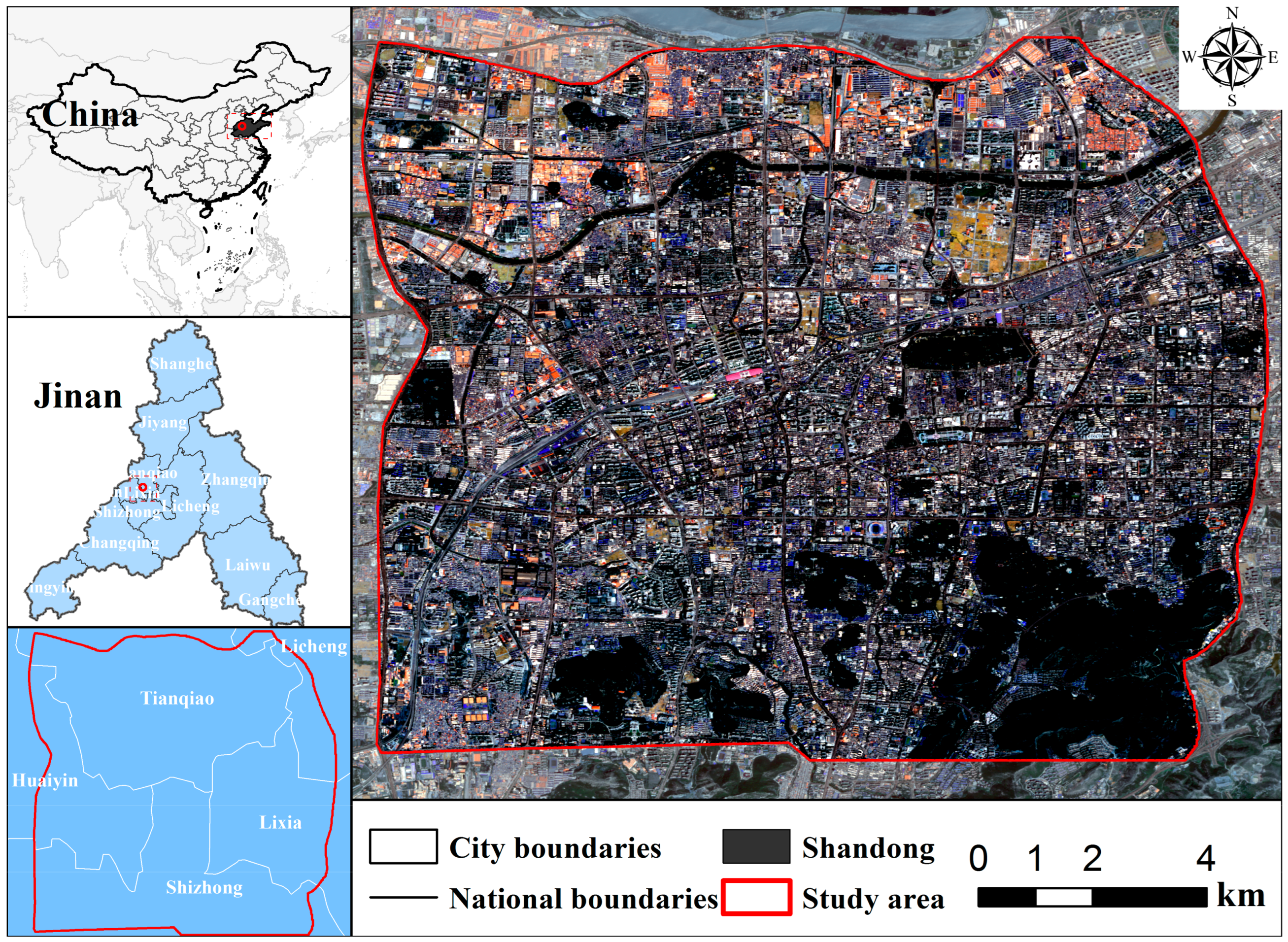
2.1. Study Area

Jinan (36°01′–37°32′ N, 116°11′–117°44′ E) is located in the middle of the North China Plain, adjacent to the Yellow River Plain in the north, and surrounded by low mountains and hills in the south. The terrain is high in the south and low in the north, and the area has a warm temperate continental monsoon climate. Jinan is one of the hottest cities in China in summer. This research took the central urban area within the second ring road of Jinan as the study area (Figure 1), covering part of Licheng, Lixia, Shizhong, Huaiyin, and Tianqiao, with an area of about 143 km². As the central area of Jinan’s urban construction and development, the urban area within the second ring road is greatly affected by heat island effects due to the rapid urban expansion, increasing agglomeration of the population, and limited space for the planning and development of construction. Therefore, choosing the area within the second ring road of Jinan as the research area has a strong research value and practical significance.

2.2. Datasets

This study used Landsat 8 OLI/TIRS remote sensing image data from the geospatial data cloud (http://www.gscloud.cn/ (accessed on 20 May 2022)), with a spatial resolution of 30 m, a revisit period of 16 days, and cloud cover of less than 5%. The satellite image transit time is approximately 10:48 a.m. Four images, taken on 27 May, 15 August, 2 October, and 19 January in 2021 were selected to represent spring, summer, autumn, and winter in the study area, respectively. See Appendix A (

Table A1. Landsat 8 image information.

Date	LANDSAT_SCENE_ID	Cloud Cover	AQI	Wind	Weather	Path/Row
2021.01.19 10:48:24	LC81220352021019LGN00	0.45%	105	Southeasterly breeze	Sunny	122/35
2021.05.27 10:47:58	LC81220352021147LGN00	0.10%	83	Southwest wind level 3	Sunny	122/35
2021.08.15 10:48:24	LC81220352021227LGN00	4.50%	68	Northeast wind level 2	Sunny	122/35
2021.10.02 10:48:38	LC81220352021275LGN00	2.21%	74	South wind level 2	Sunny	122/35

) for detailed information on the images. The 3D buildings data and green space data (Figure 2) were derived from the water flow micromap (http://www.rivermap.cn/ (accessed on 20 May 2022)), and the data are vectors. The 3D buildings data include the buildings’ ground contours and floor information. Under the assumption that the height of each floor is 3 m, the total number of floors of each building was multiplied by 3 m to obtain the buildings’ heights. The green space data include information on the green spaces’ ground contours.

3. Research Methods

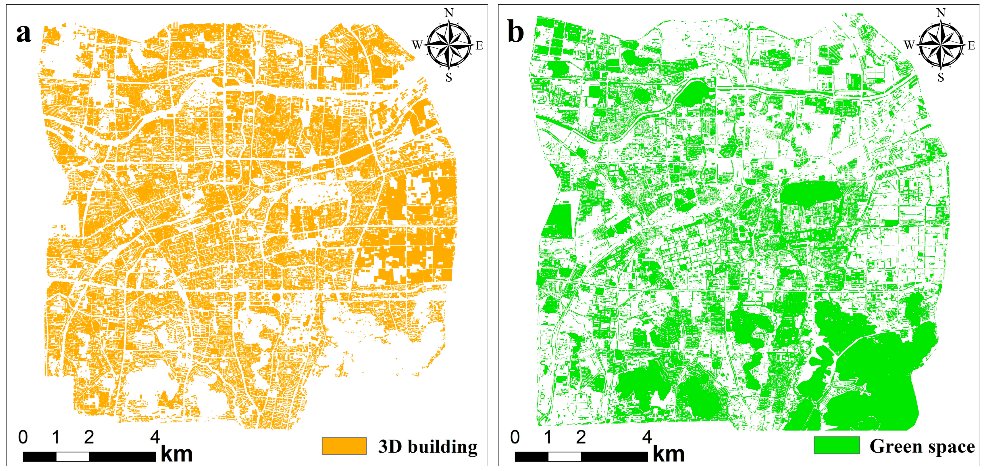
3.1. Indicators of the 3D Building and Green Space System

This research was based on the principles of generality, universality, and representativeness with reference to relevant conclusions regarding the factors influencing LST [30,31,32]. We chose a comprehensive index system of influencing factors to fully reflect the structural composition and spatial configuration of buildings and green spaces. This study focused on the individual and combined effects of 3D buildings and urban green spaces on LST. Therefore, the influential indicators were divided into two groups: (1) the nine 3D building indicators, including the average height (AH), height coefficient of variation (CH), maximum height fluctuation (AM), average volume (AV), building evenness index (BEI), building surface area (BSA), degree of spatial congestion (SCD), floor area ratio (FAR), and the building structure index (BSI); (2) the six landscape indicators of UGS, including the green coverage rate (GCR), edge density (ED), patch density (PD), largest patch index (LPI), mean patch shape index (MSI), and patch cohesion index (COHESION). All these indicators were calculated in ArcGIS10.2. See

Table 1. 3D building and green space indicators system.

Category	Indicator	Formula	Meaning
3D buildings	AH	$\mathrm{A}\mathrm{H}=\frac{1}{\mathrm{n}}{\sum }_{\mathrm{i}=1}^{\mathrm{n}}{\mathrm{H}}_{\mathrm{i}}$	Average height of building
	CH	$\mathrm{C}\mathrm{H}=\frac{1}{\mathrm{A}\mathrm{H}}{\left[\frac{1}{\mathrm{n}}{\sum }_{\mathrm{i}=1}^{\mathrm{n}}{\left({\mathrm{H}}_{\mathrm{i}}-\mathrm{A}\mathrm{H}\right)}^2\right]}^{\frac{1}{2}}$	Spatial difference of building height
	AM	$\mathrm{A}\mathrm{M}={\mathrm{H}}_{\mathrm{m}\mathrm{a}\mathrm{x}}-{\mathrm{H}}_{\mathrm{m}\mathrm{i}\mathrm{n}}$	Fluctuation degree of building height
	AV	$\mathrm{A}\mathrm{V}=\frac{1}{\mathrm{n}}{\sum }_{\mathrm{i}=1}^{\mathrm{n}}{\mathrm{V}}_{\mathrm{i}}$	Average building volume
	BEI	$\mathrm{B}\mathrm{E}\mathrm{I}=\sqrt{{\left[{\sum }_{\mathrm{i}=1}^{\mathrm{n}}\left({\mathrm{V}}_{\mathrm{i}}-\mathrm{A}\mathrm{V}\right)\right]}^2/\mathrm{A}}$	Distribution uniformity of buildings in three-dimensional space
	BSA	$\mathrm{B}\mathrm{S}\mathrm{A}=\frac{1}{\mathrm{n}}{\sum }_{\mathrm{i}=1}^{\mathrm{n}}\left({\mathrm{F}}_{\mathrm{i}}+{\mathrm{P}}_{\mathrm{i}}\times {\mathrm{H}}_{\mathrm{i}}\right)$	Average surface area of buildings
	SCD	$\mathrm{S}\mathrm{C}\mathrm{D}=\frac{{\sum }_{\mathrm{i}=1}^{\mathrm{n}}{\mathrm{V}}_{\mathrm{i}}}{{\mathrm{H}}_{\mathrm{m}\mathrm{a}\mathrm{x}}\times \mathrm{A}}\times 100\left(\mathrm{\%}\right)$	Crowding degree of buildings in 3D space
	FAR	$\mathrm{F}\mathrm{A}\mathrm{R}={\sum }_{\mathrm{i}=1}^{\mathrm{n}}\left(\frac{{\mathrm{H}}_{\mathrm{i}}}{\mathrm{C}}\times {\mathrm{F}}_{\mathrm{i}}\right)/\mathrm{A}$	Building capacity
	BSI	$\mathrm{B}\mathrm{S}\mathrm{I}=\frac{1}{\mathrm{n}}{\sum }_{\mathrm{i}=1}^{\mathrm{n}}\frac{{\mathrm{F}}_{\mathrm{i}}}{{\mathrm{H}}_{\mathrm{i}}}$	Architectural structural characteristics of buildings
Green spaces	GCR	$\mathrm{G}\mathrm{C}\mathrm{R}=\frac{{\sum }_{\mathrm{i}=1}^{\mathrm{n}}{\mathrm{G}}_{\mathrm{i}}}{\mathrm{A}}\times 100\left(\mathrm{\%}\right)$	Percentage of green patch area coverage
	ED	$ED=\frac{{\sum }_{i=1}^n{E}_i}{A}\times \mathrm{10,000}\left(\mathrm{m}/\mathrm{h}\mathrm{a}\right)$	Sum of perimeter of green patches per hectare
	PD	$PD=\frac{np}{A}\times \mathrm{10,000}\times 100\left(\mathrm{n}\mathrm{p}/{\mathrm{k}\mathrm{m}}^2\right)$	Density of green patches
	LPI	$\mathrm{L}\mathrm{P}\mathrm{I}=\frac{\mathrm{m}\mathrm{a}\mathrm{x}{\mathrm{G}}_{\mathrm{i}}}{\mathrm{A}}\times 100$	Proportion of the largest green patch in the total landscape area
	MSI	$\mathrm{M}\mathrm{S}\mathrm{I}=\frac{1}{\mathrm{n}}{\sum }_{\mathrm{i}=1}^{\mathrm{n}}\frac{{\mathrm{C}}_{\mathrm{i}}}{4\times \sqrt{{\mathrm{G}}_{\mathrm{i}}}}$	Complexity of green patch shape
	COHESION	$\mathrm{C}\mathrm{O}\mathrm{H}\mathrm{E}\mathrm{S}\mathrm{I}\mathrm{O}\mathrm{N}=\left[1-\frac{{\sum }_{\mathrm{i}=1}^{\mathrm{n}}{\mathrm{C}}_{\mathrm{i}}}{{\sum }_{\mathrm{i}=1}^{\mathrm{n}}{\mathrm{C}}_{\mathrm{i}}\sqrt{{\mathrm{G}}_{\mathrm{i}}}}\right]\times \left(1-\frac{1}{\sqrt{\mathrm{Z}}}\right)\times 100$	Physical connectivity measurement of green patches

Note: $H_i$, $V_i$, $F_i$, and $P_i$ represent the height, volume, floor area, and perimeter of the $i$th building in the grid unit, respectively; $E_i$, $G_i$, and $C_i$ represent the length, area, and perimeter of the edge segment of the $i$th green patch, respectively; $n$ is the number of buildings in the grid unit, $np$ is the number of green patches in the grid unit, $A$ is the area of the grid analysis scale cell, $C$ = 3 m, $H_{max}$ is the maximum height of the buildings in the grid cell, $H_{min}$ is the minimum height of the buildings in the grid cell, and $Z$ is the total number of cells in the analysis grid.

for the specific indicators.

3.2. Land Surface Temperature Retrieval

In this research, the land surface temperature retrieval is based on the thermal infrared radiation transfer equation [33]. First, the radiation brightness value $L_{sen}$ from the satellite based on the radiation transfer equation is calculated. Second, the corresponding brightness temperature based on the thermal radiation intensity is calculated. Finally, the brightness temperature is converted into a true surface temperature. The radiation transfer equation is represented by Equation (1) as

$$L_{sen}=B\left(T_{sen}\right)=\left[\epsilon B\right(T_s)+(1-\epsilon \left)L_d\right]\tau +L_u$$

(1)

where $L_{sen}$ is the radiation brightness from the satellite; $B$ is the Planck constant; $T_{sen}$ is the brightness temperature on the satellite, K; $\epsilon$ is the specific surface emissivity; $T_S$ is the true surface temperature, K; $\tau$ is the atmospheric transmittance; and $L_u$ and $L_d$ represent the upward and downward radiation brightness of the atmosphere, respectively. The expression of blackbody radiation brightness $B\left(T_s\right)$ is

$$B\left(T_s\right)=[L_{sen}-L_u-\tau \left(1-\epsilon \right)L_d]/\tau \epsilon$$

(2)

$T_s$ is calculated according to Planck’s formula; the formula is as follows:

$$T_s=K_2/ln\left(K_1/B\left(T_s\right)+1\right)$$

(3)

where K₁ and K₂ are radiation constants, with values 774.89 W/(m² × μm × sr) and 1321.08 K, respectively.

The radiation equation algorithm demands two parameters: the atmospheric profile parameter and surface emissivity. The atmospheric profile parameter is obtained from NASA’s web site (http://atmcorr.gsfc.nasa.gov/ (accessed on 10 May 2022)). The surface emissivity is calculated in ENVI5.3.

3.3. Analysis of the Spatial Relationships

Spatial autocorrelation was used to analyze the spatial dependence and spatial correlation characteristics of LST. The spatial autocorrelation included global autocorrelation and local autocorrelation. The global Moran’s I was used to analyze the spatial autocorrelation and aggregation of LST [34]. The formula is as follows:

$$I=\frac{\sum _{i=1}^n\sum _{j=1}^n{w}_{ij} (x_i-\stackrel{-}{x})(x_j-\stackrel{-}{x})}{S^2\sum _{i=1}^n\sum _{j=1}^n{w}_{ij}}$$

(4)

where n represents the number of pixels in the study area; $x_i$ and $x_j$ represent the urban heat island intensity of pixels $i$ and $j$, respectively; $\stackrel{-}{x}$ is the mean of all pixels in the study area; $w_{ij}$ is the spatial weight matrix; and $S$ is the standard deviation. $I$ ranges from −1 to 1. When $I$ > 0 and the Z value is significant, this indicates that LST has a positive spatial correlation. The larger $I$ is, the stronger the spatial correlation and the spatial aggregation of the intensity of heat islands will be. When $I$ < 0 and the Z value is significant, this indicates that LST has a negative spatial correlation. The smaller $I$ is, the weaker the spatial correlation and the spatial aggregation of the intensity of heat islands will be. When $I$ = 0, this indicates that LST does not have a spatial autocorrelation and the distribution presents randomness [35].

The local Moran’s I was used to further analyze the spatial heterogeneity and anomaly domain of urban heat island intensity [36]. The formula is as follows:

$$I_L=\frac{\sum _{i=1}^n\sum _{j=1}^n{w}_{ij} (x_i-\stackrel{-}{x})(x_j-\stackrel{-}{x})}{S^2}$$

(5)

When $I$ > 0 and $Z_I$ > 0, this area was classed as the “high–high cluster” type, indicating that the urban heat island intensity of this region and its adjacent regions was high and it was a hot spot. When $I$ > 0 and $Z_I$ < 0, this area was classed as the “low–low cluster” type, indicating that the urban heat island intensity of the region and adjacent regions was low. When $I$ < 0 and $Z_I$ > 0, this area was classed as the “high–low outlier” type, indicating that the high heat island intensity of the region is surrounded by a low heat island intensity of the neighboring region. When $I$ < 0 and $Z_I$ < 0, this area was classed as the “low–high outlier” type, indicating that the low heat island intensity of the region was surrounded by a high heat island intensity of the neighboring region [35].

The formula of Moran’ index is:

$$Z_I=\frac{\left[I-E\left(I\right)\right]}{\sqrt{Var\left(I\right)}}$$

(6)

where $Z_I$ can judge the significance of the Moran index, $E\left(I\right)$ is the expected value of Moran’s index, and $Var\left(I\right)$ is the variance of Moran’s exponent.

The data used in this study were typical geospatial data, and there was a level of spatial dependence among the data. The spatial regression model corrected the spatial dependence problem and accurately analyzed the correlation between LST and the influencing factors. The spatial regression model included the spatial lag model (SLM) and the spatial error model (SEM). The SEM model is more suitable when there is spatial dependence in the random error term [37]. It is expressed by Equation (7) as follows:

$$y=x\beta +\lambda w_u+\epsilon , \epsilon ~N (0,{\delta }^2)$$

(7)

where $y$ is the matrix of the dependent variable (LST); $x$ is the influencing factor matrix; $\lambda$ is the coefficient of the independent variable; $\beta$ is the parameter matrix; $w_u$ is the spatial weight matrix; and $\epsilon$ is the spatial error term.

3.4. Boosted Regression Tree Model (BRT)

This research used the BRT model to calculate the marginal utility of the indicators on changes in LST. We implemented the BRT model based on the R language platform, and used the packages “gbm” and “demo” in the R software. The dependent variable was based on the LST in the grid cell, and the independent variable was the indicator of the influencing factor. The BRT model is a supervised learning method that requires specifying three parameters: learning rate, tree complexity, and bagging score. After debugging, the final parameters in the BRT model were set with a learning rate of 0.005, a tree complexity of 5, and a bagging score of 0.5 [1,38]. In addition, the BRT model uses 10x cross validation and 50% training data to select the optimal model. The correlation of the model data test set is 0.58, and the correlation of the model data training set is 0.55. It is expressed by Equation (8) as follows:

$$fm(x)={\sum }_{i=1}^{m}T(x;Q)$$

(8)

where $T(x;Q)$ represents the decision tree; $m$ represents the number of trees; and $Q$ represents the parameters of the decision tree.

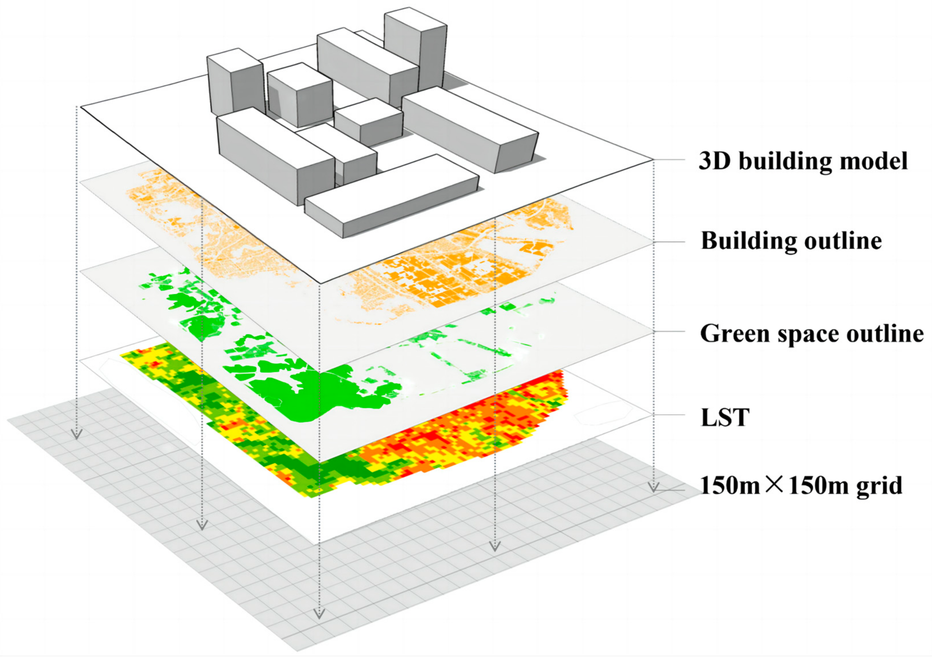
3.5. Data Integration and Modeling

The multisource data used in the study had different spatial resolutions, so the appropriate way to standardize the data was to overlay them into a uniform regular grid. The patterns and spatial distribution of geographical research objects are scale-dependent. Under different spatial scales, the influence of 3D buildings and green spaces on LST may be different. If the scale is too small, the correlation analysis between the landscape index and LST will be divided into multiple grid correlations, while if the scale is too large, the detailed relationships of spatial features cannot be reflected. Therefore, a reasonable scale should be selected during the analysis. According to the conclusions on the scale effect of the surface’s thermal environment [39,40] and the resolution of the image data, 150 m was chosen as the appropriate spatial scale. Therefore, we chose 150 m as the spatial analysis scale. Firstly, this study used the ArcGIS fishing net tool to create a 150 m spatial scale fishing net to divide the research units. Secondly, we resampled the surface temperature data obtained from the Landsat 8 inversion to 150 m. Finally, we used the GIS spatial analysis method to overlay the surface temperature data, 3D building data, and urban green space data into a unified regular fishing net for subsequent quantitative analysis (Figure 3).

4. Results

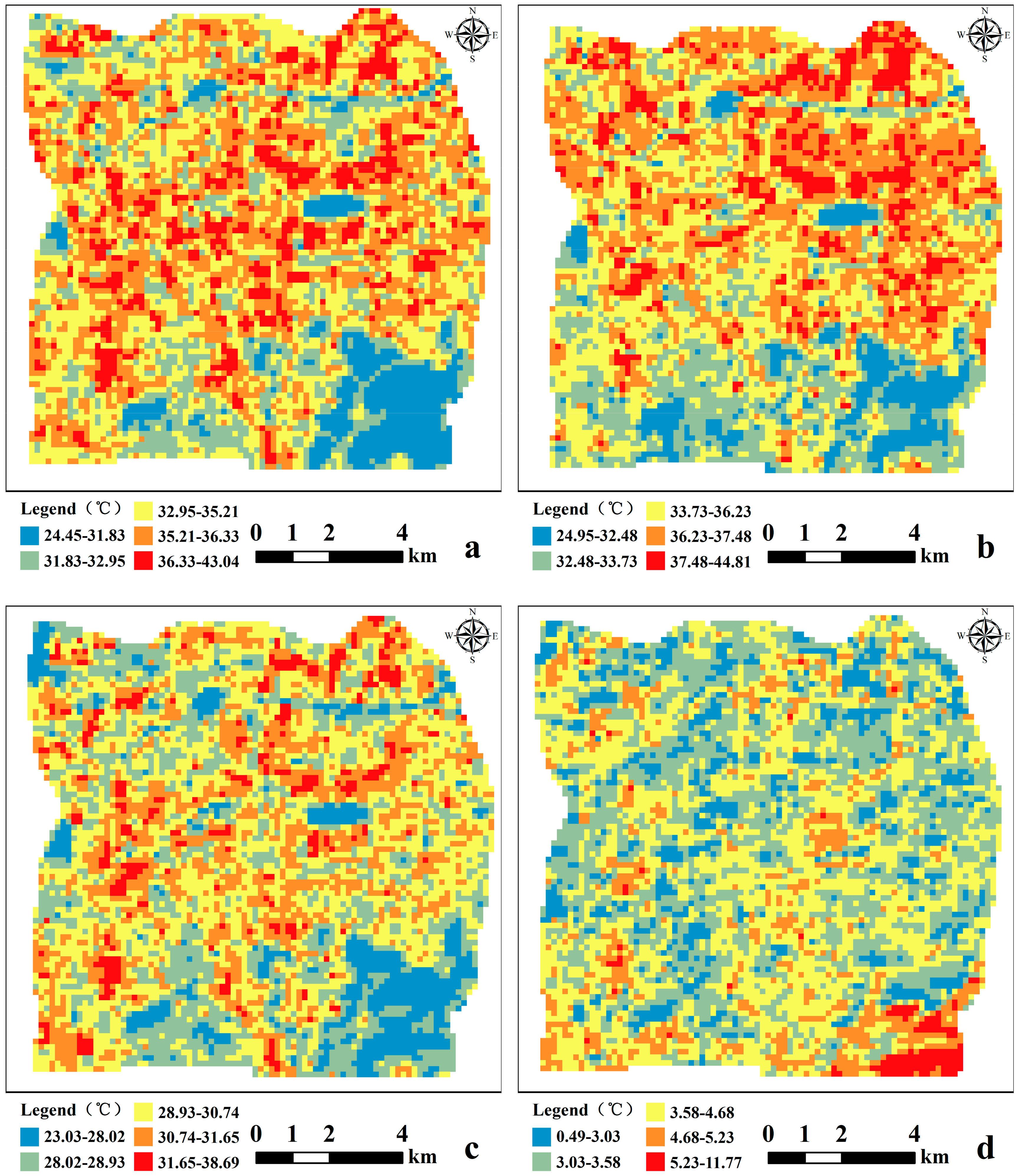
4.1. Temporal and Spatial Distribution of LST

This research used the mean standard deviation method [41] to divide the heat island intensity into five grades (strong cold island, cold island, mesothermal island, heat island, strong heat island). Among them, strong cold island and cold island are defined as cold island patches, and heat island and strong heat island are defined as heat island patches. From the perspective of seasonal changes (

Table 2. Statistical table of heat island intensity rates for spring, summer, autumn, and winter.

Season	Strong Cold Island	Cold Island	Mesothermal Island	Heat Island	Strong Heat Island	Average LST (°C)	Standard Deviation
Spring (May)	14.92%	10.51%	42.07%	19.74%	12.76%	34.08	2.25
Summer (June)	15.64%	11.56%	39.64%	19.46%	13.70%	34.98	2.50
Autumn (October)	14.70%	13.56%	42.43%	15.50%	13.81%	29.84	1.82
Winter (January)	12.43%	15.37%	46.89%	14.61%	10.70%	4.13	1.10

), the highest proportion of hot island patches (33.16%) was in summer, followed by spring and autumn, and the lowest (25.31%) was in winter. The heat island effect was most pronounced in summer, with significant temperature differences and an average LST of 34.98 °C. The proportion of cold island patches was highest in autumn, followed by winter, summer, and spring. Figure 4 shows the seasonal variations in the spatial distribution of the thermal environment. There were differences in the size of heat island patches and cold island patches in the four seasons. In summer, the urban heat island profile was the most pronounced, with the core of the city showing a clear concentration of high temperatures and a spatial pattern characterized by a connected concentration and spreading nearby. This was mainly located in the southeastern part of Tianqiao District, the western part of Lixia District, and the eastern part of Huaiyin District, especially in dense industrial and commercial areas. The area has a dense architectural environment, high population density, and low green space coverage, and the land cover is mainly made of impervious materials such as brick and asphalt, so the heat island effect is very significant. The cold island patches were mainly distributed in Qianfo Mountain Scenic Area, Daming Lake Park, Xiaoqing River, and other water and forest areas, showing the spatial pattern of being generally dispersed and locally concentrated. It is worth noting that the LST in the southern mountain area was relatively high in winter, which may be due to the differences in thermodynamics caused by the different underlying surfaces. Compared with bare land, vegetation has a larger specific heat capacity and can store more heat, and the temperature drop is moderate. Therefore, the surface temperature was relatively high. The research results indicated that large green spaces with high connectivity and aggregation had more prominent cooling effects. On the contrary, highly clustered urban buildings had a more severe heating effect.

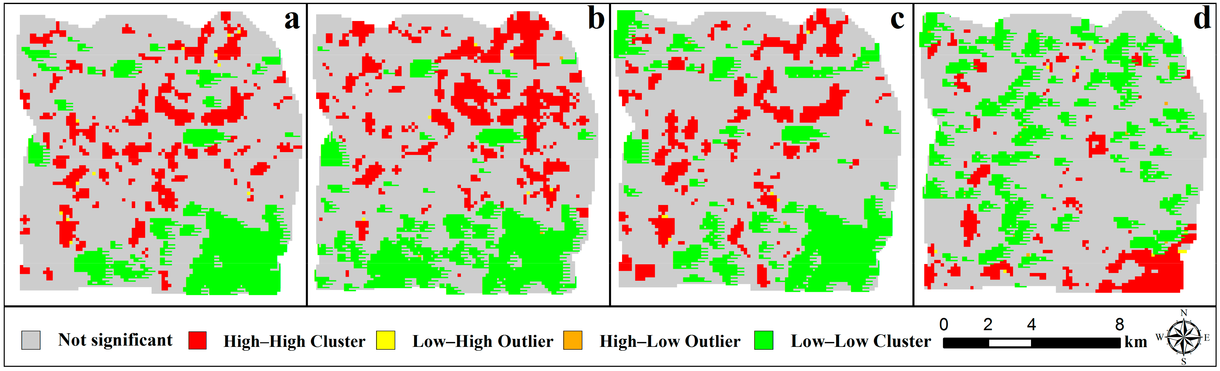
4.2. Spatial Autocorrelation of LST

The global Moran’s I was used to quantitatively characterize the spatial autocorrelation of urban heat island intensity, as shown in

Table 3. Global autocorrelation statistics of LST in the four seasons.

Index	Spring (May)	Summer (June)	Autumn (October)	Winter (January)
Global Moran’s I	0.77 **	0.78 **	0.74 **	0.69 **
Z scores	87.22	87.84	83.41	77.75

Note: ** indicates p < 0.01.

. It can be seen that the values of the global Moran’s I were all positive, with p < 0.01, indicating that the LST presented a significant spatial agglomeration. Among the seasons, the spatial agglomeration of urban heat island intensity in summer was the most significant, followed by spring, and the spatial agglomeration in autumn and winter was relatively weak.

This research used the local Moran’s I to test the correlation between the intensity of local heat islands and the neighboring space. We calculated the proportion of different aggregation categories, and the results are shown in

Table 4. Local autocorrelation statistics of LST in the four seasons.

Season	High–High Cluster	Low–Low Cluster	High–Low Outlier	Low–High Outlier
Spring (May)	14.17%	13.11%	0.01%	0.19%
Summer (June)	16.34%	15.20%	0.05%	0.09%
Autumn (October)	13.17%	14.06%	0.05%	0.09%
Winter (January)	8.85%	12.31%	0.22%	0.13%

. The proportion of “high–high cluster” areas, namely areas with highly aggregated urban heat island intensity, increased from spring to summer (16.34%), reached a peak, and gradually decreased; winter (8.85%) had the lowest proportion. “Low–low cluster” refers to areas with low aggregation of urban heat island intensity, with the highest proportion in summer, followed by autumn, spring, and winter. It can be seen from Figure 5 that the spatial distribution of local autocorrelation and LST had some similarity. The “high–high cluster” areas are mainly distributed to the east of the west second ring road, the south of Tianqiao District, the west of Lixia District, and other high–density low–rise built-up areas. The artificial materials such as buildings and impervious surfaces in the area had low albedo, strong impermeability, and high heat island intensity. The “low–low cluster” pattern was mainly found in forested areas such as mountainous woodlands and water parks, where green vegetation is spread over a large area and has a complex shape. The vegetation is dominated by arbors, and its vegetation height, leaf shape, and crown shape can provide greater canopy density, with a more pronounced cooling effect [42]. The proportion of “high–low outlier” and “low–high outlier” outliers did not exceed 1%. This research showed that the LST in the region had significant spatial aggregation features and spillover effects. Areas with highly agglomerated urban heat islands were mainly concentrated in high-density built-up areas with dense buildings and a crowded population.

4.3. Quantitative Relationship between 3D Building/Green Space and LST

4.3.1. Spatial Regression Analysis

According to the results above, summer had the most significant urban heat island effect, and many studies have proven that summer is the best season for discussing the urban thermal environment [43,44]. Meanwhile, as an important part of the urban landscape, urban buildings and green spaces are of great significance for analyzing their spatial configuration to alleviate the heat island effect. Therefore, the follow-up part of the study mainly focused on the impact of urban buildings and green spaces on the LST in summer.

On the basis of the spatial regression model, we analyzed the contribution of 3D buildings and green space indicators to the LST, as shown in Figure 6. In the group of 3D building indicators (Figure 6a), the leading indicators affecting the LST were SCD and BSA, contributing 22.6% and 19.3%, respectively, indicating that SCD and BSA had a significant positive correlation with LST and had a significant heating effect on cities. The second-ranked indicators were CH, AV, and AH, contributing 14.6%, 13.3%, and 12.6%, respectively. CH and AV were positively correlated with LST, while AH was negatively correlated with it, indicating that tall and thin buildings with small differences in height can alleviate the heat island effect to a certain extent. The impacts of AM, FAR, BEI, and BSI on LST were far lower than those of the first five indicators, contributing 7.3%, 5.3%, 4.7%, and 0.3%, respectively. In the green space indicator group (Figure 6b), LPI, GCR, and ED were significantly negatively correlated with LST, with relative contributions of 35.4%, 27.1%, and 27.1%, respectively. The cooling effect of green spaces can be effectively improved by reasonably adjusting the green spaces’ areas and perimeters. PD and COHESION were positively correlated with LST, while MSI was negatively correlated with LST, with relative contributions of 8.3%, 1.7%, and 0.4%, respectively, indicating that the large patches of green space in the region had better cooling benefits than the scattered patches. In the group of combined indicators (Figure 6c), SCD had the greatest influence on LST, with its relative contribution being as high as 24.7%, followed by BSA, CH, GCR, AV, and AH, for which the relative contributions were 12.8%, 12.4%, 11.9%, 7.1%, and 6.7%, respectively. The other indicators had a small impact, indicating that these six indicators were the key factors affecting the heat island effect. Therefore, in the process of urban development, the height of buildings should be appropriately increased and the floor area of buildings and the crowding degree of buildings should be reduced as much as possible. Vertical expansion should be used instead of horizontal expansion to keep the direction of adjacent buildings consistent, and the difference in height should not be too large, thus forming a connected urban ventilation corridor. At the same time, authorities should establish a green space network system with complete functions and a clear structure to minimize UHIs.

Figure 6d shows the relative contribution of the six main indicators to LST. We deleted nine indicators that had no significant effect on the LST (contribution value < 8%, p > 0.05), and focused on the analysis of the relative contributions and marginal utility of the leading indicators on LST. The results showed that SCD was the most influential indicator on LST, with a relative contribution of 33.1%, which was far greater than that of the other five indicators, indicating that SCD was the decisive factor affecting LST. GCR was the only greenbelt indicator in the group of leading indicators, with a relative contribution of 15.9%. Compared with the impact on LST alone, the relative contribution of greenbelt indicators was significantly lower. The cooling effect of green spaces will be limited by three-dimensional buildings to a certain extent. Among the six leading indicators, even when the cooling effects of green spaces were considered, 3D building indicators still explained up to 84.1% of the change in the LST, which further indicated that 3D buildings are the decisive factor affecting LST. Although green spaces can alleviate the thermal environment to some extent, the key is to optimize the 3D spatial configuration of buildings.

4.3.2. Analysis of Marginal Utility

The marginal utility analyzes the influence of independent variables on dependent variables by maintaining the mean value of variables. We use the BRT model to draw a marginal utility curve to further analyze the potential impact of the leading indicators on LST (Figure 7). Among the six leading indicators, SCD was positively correlated with LST, and LST increased significantly with an increase in SCD. When SCD < 60%, LST increased by about 0.38 °C for every 10% increase in SCD. When the SCD ratio exceeded 60%, the warming effect of SCD on LST was no longer significant. The warming effect of BSA on LST was obvious. LST increased by 0.18 °C for every 10% increase in BSA. When the BSA exceeded 4286 m², changes in LST tended to be stable. GCR was negatively correlated with the changes in LST. When GCR > 44%, LST decreased significantly with an increase in GCR. When GCR > 62%, this provided a 1.1 °C cooling effect, but beyond this threshold, the cooling effect did not increase significantly. Among the six leading indicators, AH was the only 3D building indicator that had a negative impact on LST. When AH increased by 10%, this provided a cooling effect of 0.1 °C. When AH reached 20 m, the cooling effect was no longer significant. CH and AV were positively correlated with LST, and the warming effect was relatively small. Within the threshold range, LST increased by about 0.08 °C and 0.07 °C for every 10% increase in these factors.

5. Discussion

5.1. Quantitative Relationship between 3D Buildings and LST

The heat balance mechanism in the 3D space of buildings is complex. It is extremely important to fully understand the impact mechanism of urban 3D buildings on LST for optimizing building patterns, alleviating the heat island effect, and promoting the sustainable development of the city. In this study, we found that SCD and BSA had a significant impact on the thermal environment. Crowded spaces and large building groups usually lack a fully connected urban ventilation corridor, which affects the speed and flow of wind and heat transfer, so it has a significant warming effect on the city. The positive correlation of CH and AV with LST has been widely demonstrated [45]. The larger a building is, the more human activities it can accommodate, and thus the more heat it can generate. Height differences can change the surface roughness of mechanical turbulence and affect convective heat dissipation. The study also found that scattered high-rise buildings can lower LST compared with compact low-rise buildings. Increasing the buildings’ height can produce good cooling effects. When AH < 20 m, every 10% increase could provide a 0.1 °C cooling effect, which is similar to the conclusions of [46]. Tall and thin buildings with a small height difference can enhance convective heat dissipation and alleviate the heat island effect to a certain extent. Meanwhile, the shadows of tall buildings effectively block out solar radiation and provide partial cooling, thus producing lower temperatures than near the surrounding low-rise buildings [47]. AM, BEI, and BSI had relatively little influence on LST. This may be because these indicators integrate building height, density, area and other information, so their impact on LST may vary. In addition, we found that FAR, as a comprehensive planning indicator for urban development, made a small contribution to LST. This may be due to the fact that buildings with a larger FAR usually occupy a larger foundation area and have a greater vertical height, which have a counter-effect on the LST and reduce the contribution of the FAR to the LST [48].

5.2. Quantitative Relationship between Green Space and LST

Green spaces absorb heat through shading and transpiration, which can effectively improve the thermal environment. Therefore, it is of great theoretical significance and practical value to optimize the layout of green spaces so that the limited area of green spaces can have a greater cooling effect. This study found that when GCR > 44%, the cooling effect on the LST improved significantly, and when GCR > 62%, a cooling effect of 1.1 °C could be provided. Beyond this threshold, the cooling effect was no longer significant. Ref. [49] also showed that within the threshold range, increasing the green coverage would significantly improve the cooling effect. LST was negatively correlated with LPL and ED. Increasing the area and perimeter of green spaces can strengthen the penetration and connection between green space patches and the surrounding ecological patches (water bodies and green space), increase the heat transfer with the external environment, and produce a good cooling effect, which is consistent with the conclusions of [50]. In theory, PD is negatively correlated with LST due to the increased chance of heat transfer with the external environment. However, the study concluded that PD was positively correlated with LST. The reason may be that in areas with high patch density, green spaces are usually fragmented and dispersed, while fragmented patches are more susceptible to the impact of the surrounding thermal environment, reducing the cooling effect of the greenbelt to some extent. LST was negatively correlated with MSI. Li et al. also reached similar conclusions [27]. The heat island intensity tends to be low in areas with complex shapes of green space. Green space patches in this pattern have more edges, which can provide greater shade and promote the circulation of heat between the surrounding environment and the green space, so that the overall temperature is lower. However, some research results have contradicted each other. Ref. [51] found that the simpler the shape of green spaces, the better the cooling effect. The correlation between the urban green space index and the heat island effect was different in different studies. On the one hand, the results calculated for the landscape index may be different due to the different spatial resolution of the remote sensing images extracted from green spaces. On the other hand, the final results may be different due to the different methods used for measuring the heat island effect [52].

5.3. The Combined Impact of 3D Buildings and Green Spaces on LST

The heat balance mechanism inside a city is very complicated. Expansion of urban buildings will affect the surface energy balance and aggravate the heat island effect. Green spaces can form a cold island effect through transpiration, shading, and heat absorption. It is of great significance to explore how architecture and green spaces affect LST together, to realize the strong coupling of the artificial environment and green spaces, to alleviate the heat island effect. This study found that among the 15 indicators, SCD had the greatest influence on LST, and its contribution is far higher than that of the other indicators, followed by BSA and CH. Even considering green spaces, the contribution value of this indicator to LST still ranks in the top three. This shows that crowded spaces and large building groups will affect air flow and heat transfer, and exacerbate the heat island effect, which is the main reason for the rise in surface temperatures. As the only green space indicator among the leading indicators (contribution value > 8%), the relative contribution value of GCR to LST was 11.9%, which decreased by 15.2% compared with the independent influence of GCR on LST, indicating that the greenbelt cooling effect was limited by 3D buildings. At the same time, we found that nine building indicators explained 75.5% of the change in LST, while the six green space indicators could only explain 25.5% of the change in LST, and the cooling effect of LPI and ED were no longer significant. This showed that 3D buildings have enormous implications on the greenbelt cooling effect, and the cooling effect is significantly less than the heating effect of buildings on the surrounding environment. We analyzed the combined influence of 15 indicators on LST. The results showed that it is far from enough to rely on green spaces to mitigate the UHI effect when 3D buildings are densely distributed and space is crowded. The key is to rationally plan the 3D spatial structure of the city.

5.4. Limitations and Prospects

This study focuses on the impact mechanism and change rule of 3D buildings and green spaces on the LST, which has certain guiding significance for urban landscape pattern optimization and thermal environment mitigation. However, current research still has certain limitations. First, the index system of urban green spaces needs to be improved further. Due to data limitations, some indicators have not been discussed. For example, the cooling effect of vegetation may be associated with tree species and height [53]. Secondly, the research mainly focused on exploring the impact mechanism of UHIs or the cooling mitigation strategies for green spaces [54]. The selection of indicators focuses on biophysical factors, with low emphasis on humanistic and social factors, and in-depth research on the regulation mechanism of the urban thermal environment has not yet been performed [55]. Third, the mechanism of dynamic changes and the future trends of the impact of 3D buildings and green spaces on LST have not been discussed. Therefore, future research should concentrate mainly on: (1) constructing a more reasonable impact indicator system to accurately analyze the impact mechanism of 3D buildings and urban green spaces on LST; (2) establishing an evaluation indicator system for thermal environment regulation services, and analyzing the comprehensive demand level of the audience for thermal environment regulation services and the supply capacity of green infrastructure for regulating the thermal environment; (3) exploring the mechanism of dynamic changes and future trends between the influencing indicators and the heat island effect.

6. Conclusions

This research used a spatial regression model and the BRT model to analyze and compare the impact mechanism and change rule of buildings and green spaces on the LST. The main conclusions are as follows:

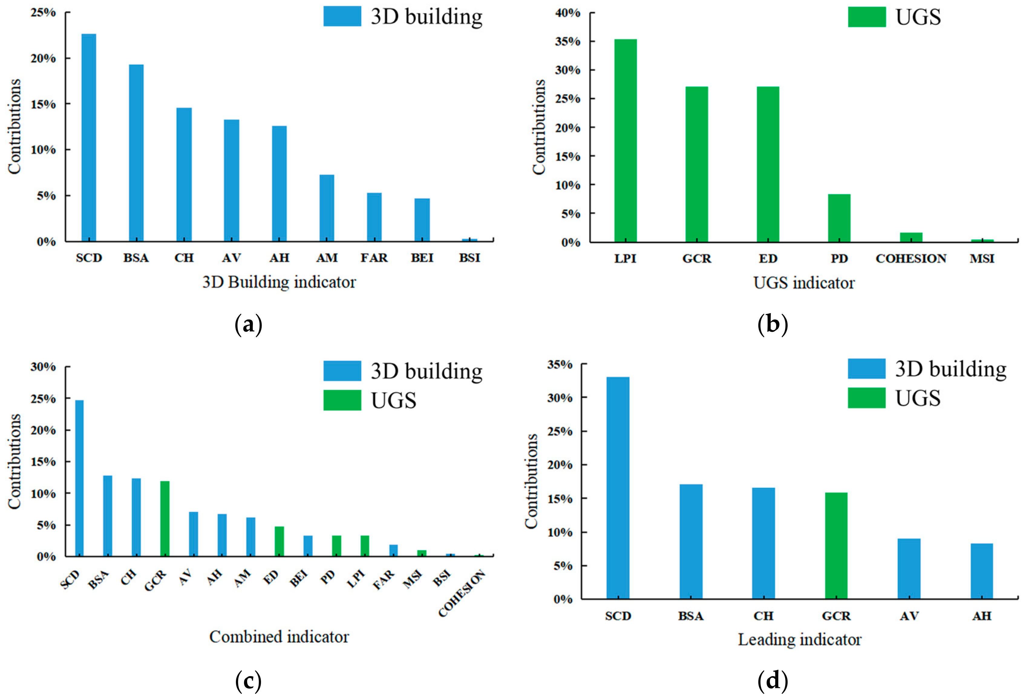
• Among the 3D building indicators, SCD and BSA were the leading indicators affecting LST, with contributions of 22.6% and 19.3%, respectively. Among the green space indicators, LPI, GCR, and ED were significantly negatively correlated with LST, with relative contributions of 35.4%, 27.1%, and 27.1%, respectively. Among the combined indicators, SCD was the most influential indicator, with a contribution of 24.7%, far exceeding that of other indicators. The urban thermal environment can be effectively alleviated by reducing building congestion and floor area and reasonably adjusting the area, perimeter, and shape of green spaces.
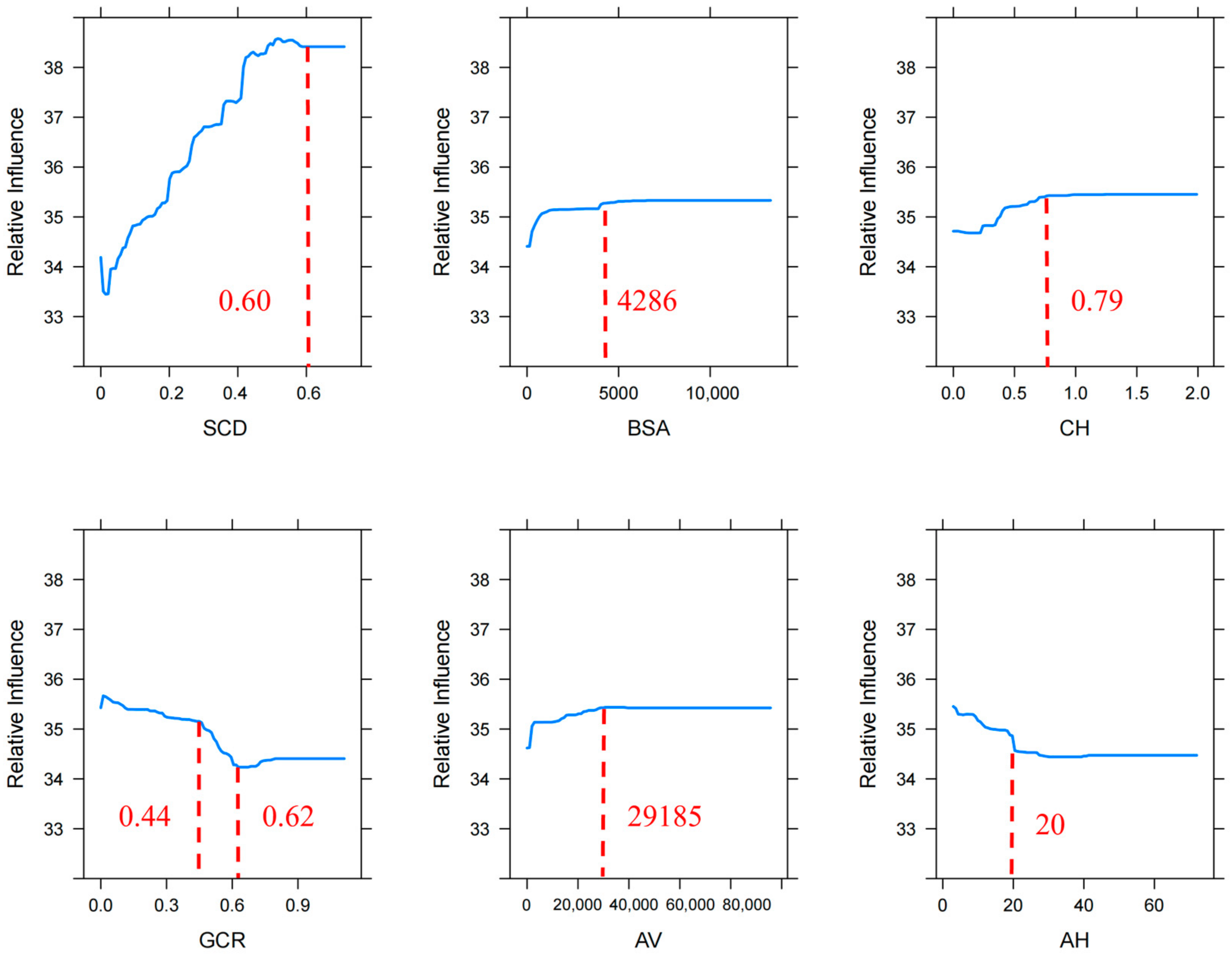
• Among the six leading indicators, SCD and LST were positively correlated. When the SCD was less than 60%, LST increased by 0.38 °C for every 10% increase. BSA had some heating effect on the LST; within the threshold range, the LST increased by 0.18 °C for every 10% increase. GCR was negatively correlated with LST. When GCR > 44%, the LST decreased significantly with an increase in GCR. When GCR > 62%, it could provide a cooling effect of 1.1 °C. The composition and configuration of urban landscapes should fully consider the cooling threshold of indicators to maximize the mitigation of LST.
• Among the 15 combined indicators, even considering the cooling effect of UGS, the building indicators could still explain 75.5% of the variation in LST. The six green space indicators explained 24.5% of the change in LST, but their contribution was significantly lower than their individual impacts on LST. Dense buildings will limit the greenbelt cooling effect to some extent. The key to mitigating UHIs is to rationally configure and optimize the spatial structure of 3D buildings.

References

1. Yuan, B.; Zhou, L.; Dang, X.; Sun, D.; Hu, F.; Mu, H. Separate and combined effects of 3D building features and urban green space on land surface temperature. J. Environ. Manag. 2021, 295, 113116. [Google Scholar] [CrossRef] [PubMed]
2. Meng, X.; Meng, F.; Zhao, Z.; Yin, C. Prediction of Urban Heat Island Effect over Jinan City Using the Markov-Cellular Automata Model Combined with Urban Biophysical Descriptors. J. Indian Soc. Remote Sens. 2021, 49, 997–1009. [Google Scholar] [CrossRef]
3. Zhao, L.; Lee, X.; Smith, R.B.; Oleson, K. Strong contributions of local background climate to urban heat islands. Nature 2014, 511, 216–219. [Google Scholar] [CrossRef]
4. Huang, X.J.; Wang, B.; Liu, M.M.; Guo, Y.H.; Li, Y.Y. Characteristics of urban extreme heat and assessment of social vulnerability in China. Geogr. Res. 2020, 39, 1534–1547. [Google Scholar]
5. Xv, X.Z.; Zheng, Y.F.; Yin, J.F.; Wu, R.J. Characteristics of high temperature and heat wave in Nanjing City and their impacts on human health. Chin. J. Ecol. 2011, 30, 2815–2820. [Google Scholar]
6. He, B.-J.; Zhao, D.; Dong, X.; Xiong, K.; Feng, C.; Qi, Q.; Darko, A.; Sharifi, A.; Pathak, M. Perception, physiological and psychological impacts, adaptive awareness and knowledge, and climate justice under urban heat: A study in extremely hot-humid Chongqing, China. Sustain. Cities Soc. 2022, 79, 103685. [Google Scholar] [CrossRef]
7. Patz, J.A.; Campbell-Lendrum, D.; Holloway, T.; Foley, J.A. Impact of regional climate change on human health. Nature 2005, 438, 310–317. [Google Scholar] [CrossRef]
8. Wang, J.Y.; Meng, F.; Fu, P.J.; Jin, F.X. Investigating the Coupling of Supply and Demand for Urban Blue and Green Spaces’ Cooling Effects in Shandong, China. Atmosphere 2023, 14, 404. [Google Scholar] [CrossRef]
9. Wang, X.; Li, H.; Sodoudi, S. The effectiveness of cool and green roofs in mitigating urban heat island and improving human thermal comfort. Build. Environ. 2022, 217, 109082. [Google Scholar] [CrossRef]
10. He, B.-J.; Zhao, D.; Xiong, K.; Qi, J.; Ulpiani, G.; Pignatta, G.; Prasad, D.; Jones, P. A framework for addressing urban heat challenges and associated adaptive behavior by the public and the issue of willingness to pay for heat resilient infrastructure in Chongqing, China. Sustain. Cities Soc. 2021, 75, 103361. [Google Scholar] [CrossRef]
11. Ulpiani, G. Water mist spray for outdoor cooling: A systematic review of technologies, methods and impacts. Appl. Energy 2019, 254, 113647. [Google Scholar] [CrossRef]
12. Shi, Z.; Yang, J.; Zhang, Y.; Xiao, X.; Xia, J.C. Urban ventilation corridors and spatiotemporal divergence patterns of urban heat island intensity: A local climate zone perspective. Environ. Sci. Pollut. Res. 2022, 29, 74394–74406. [Google Scholar] [CrossRef]
13. Dewan, A.; Kiselev, G.; Botje, D.; Mahmud, G.I.; Bhuian, M.H.; Hassan, Q.K. Surface urban heat island intensity in five major cities of Bangladesh: Patterns, drivers and trends. Sustain. Cities Soc. 2021, 71, 102926. [Google Scholar] [CrossRef]
14. Wang, C.; Wang, Z.-H.; Kaloush, K.E.; Shacat, J. Perceptions of urban heat island mitigation and implementation strategies: Survey and gap analysis. Sustain. Cities Soc. 2021, 66, 102687. [Google Scholar] [CrossRef]
15. Ma, Y.; Zhao, M.; Li, J.; Wang, J.; Hu, L. Cooling Effect of Different Land Cover Types: A Case Study in Xi’an and Xianyang, China. Sustainability 2021, 13, 1099. [Google Scholar] [CrossRef]
16. Luo, X.; Yang, J.; Sun, W.; He, B. Suitability of human settlements in mountainous areas from the perspective of ventilation: A case study of the main urban area of Chongqing. J. Clean. Prod. 2021, 310, 127467. [Google Scholar] [CrossRef]
17. Tian, Y.; Zhou, W.; Qian, Y.; Zheng, Z.; Yan, J. The effect of urban 2D and 3D morphology on air temperature in residential neighborhoods. Landsc. Ecol. 2019, 34, 1131–1178. [Google Scholar] [CrossRef]
18. Chen, Q.; Cheng, Q.H.; Chen, Y.H.; Li, K.N.; Jing, C.F. Analysis of the influence of the urban building skyview factor on landsurface thermal environment. Sci. Surv. Mapp. 2021, 46, 148–155. [Google Scholar]
19. van Vliet, J. Direct and indirect loss of natural area from urban expansion. Nat. Sustain. 2019, 2, 755–763. [Google Scholar] [CrossRef]
20. Giannopoulou, K.; Santamouris, M.; Livada, I.; Georgakis, C.; Caouris, Y. The Impact of Canyon Geometry on Intra Urban and Urban: Suburban Night Temperature Differences Under Warm Weather Conditions. Pure Appl. Geophys. 2010, 167, 1433–1449. [Google Scholar] [CrossRef]
21. Hu, L.; Li, Q. Greenspace, bluespace, and their interactive influence on urban thermal environments. Environ. Res. Lett. 2020, 15, 034041. [Google Scholar] [CrossRef]
22. Gao, J.; Gong, J.; Li, J.Y. Effects of source and sink landscape pattern on land surface temperature: An urban heat island study in Wuhan City. Prog. Geogr. 2019, 38, 1770–1782. [Google Scholar] [CrossRef]
23. Jiang, Y.F.; Huang, J. Quantitative Analysis of Mitigation Effect of Urban Blue—Green Spaces on Urban Heat Island. Resour. Environ. Yangtze Basin 2022, 31, 2060–2072. [Google Scholar]
24. Kong, F.; Yin, H.; James, P.; Hutyra, L.R.; He, H.S. Effects of spatial pattern of greenspace on urban cooling in a large metropolitan area of eastern China. Landsc. Urban Plan. 2014, 128, 35–47. [Google Scholar] [CrossRef]
25. Chen, A.; Sun, R.; Chen, L. Effects of urban green pattern on urban surface thermal environment. Acta Ecol. Sin. 2013, 33, 2372–2380. [Google Scholar] [CrossRef]
26. Li, B.; Wang, W.; Bai, L.; Chen, N. Effects of spatio-temporal landscape patterns on land surface temperature: A case study of Xi’an city, China. Environ. Monit. Assess. 2018, 190, 419. [Google Scholar] [CrossRef]
27. Li, X.; Zhou, W. Optimizing urban greenspace spatial pattern to mitigate urban heat island effects: Extending understanding from local to the city scale. Urban For. Urban Green. 2019, 41, 255–263. [Google Scholar] [CrossRef]
28. Du, H.; Cai, W.; Xu, Y.; Wang, Z.; Wang, Y.; Cai, Y. Quantifying the cool island effects of urban green spaces using remote sensing Data. Urban For. Urban Green. 2017, 27, 24–31. [Google Scholar] [CrossRef]
29. Lai, D.Y.; Liu, W.Y.; Gan, T.T.; Liu, K.X.; Chen, Q.Y. A review of mitigating strategies to improve the thermal environment and thermal comfort in urban outdoor spaces. Sci. Total Environ. 2019, 661, 337–353. [Google Scholar] [CrossRef]
30. Yu, X.; Liu, Y.; Zhang, Z.; Xiao, R. Influences of buildings on urban heat island based on 3D landscape metrics: An investigation of China’s 30 megacities at micro grid-cell scale and macro city scale. Landsc. Ecol. 2021, 36, 2743–2762. [Google Scholar] [CrossRef]
31. Chen, A.; Yao, L.; Sun, R.; Chen, L. How many metrics are required to identify the effects of the landscape pattern on land surface temperature? Ecol. Indic. 2014, 45, 424–433. [Google Scholar] [CrossRef]
32. Chen, J.; Zhan, W.; Jin, S.; Han, W.; Du, P.; Xia, J.; Lai, J.; Li, J.; Liu, Z.; Li, L.; et al. Separate and combined impacts of building and tree on urban thermal environment from two- and three-dimensional perspectives. Build. Environ. 2021, 194, 107650. [Google Scholar] [CrossRef]
33. Weng, Q.; Lu, D.; Schubring, J. Estimation of land surface temperature–vegetation abundance relationship for urban heat island studies. Remote Sens. Environ. 2004, 89, 467–483. [Google Scholar] [CrossRef]
34. Moran, P.A.P. The Interpretation of Statistical Maps. J. R. Stat. Soc. Ser. B (Methodol.) 1948, 10, 243–251. [Google Scholar] [CrossRef]
35. Xiang, Y.; Zhao, Z.X. Analysis of Driving Factors of Urban Heat Island Based on Geographical Detector: Taking Wuhan City as an Example. Resour. Environ. Yangtze Basin 2020, 29, 1768–1779. [Google Scholar]
36. Anselin, L. Local indicators of spatial association—LISA. Geogr. Anal. 1995, 27, 93–115. [Google Scholar] [CrossRef]
37. Xiao, R.; Liu, Y.; Huang, X.; Shi, R.; Yu, W.; Zhang, T. Exploring the driving forces of farmland loss under rapidurbanization using binary logistic regression and spatial regression: A case study of Shanghai and Hangzhou Bay. Ecol. Indic. 2018, 95, 455–467. [Google Scholar] [CrossRef]
38. Elith, J.; Leathwick, J.; Hastie, T. A Working Guide to Boosted Regression Trees. J. Anim. Ecol. 2008, 77, 802–813. [Google Scholar] [CrossRef]
39. Jiang, Y.H.; Jiao, L.M.; Zhang, B.E. Scale effect of the spatial correlation between urban land surface temperature and NDVI. Prog. Geogr. 2018, 37, 1362–1370. [Google Scholar]
40. Yv, X.Y.; Xv, G.; Liu, Y.; Xiao, R. Influences of 3D features of buildings on land surface temperature: A case study in the Yangtze River Delta urban agglomeration. China Environ. Sci. 2021, 41, 5806–5816. [Google Scholar]
41. Chen, S.L.; Wang, T.X. Comprison analyses of equal interval method and mean-standard deviation method used to delimitate urban heat island. J. Geo-Inf. Sci. 2009, 11, 145–150. [Google Scholar]
42. Kong, F.H.; Yan, W.J.; Zheng, G.; Yin, H.W.; Cavan, G.; Zhan, W.F.; Zhang, N.; Cheng, L. Retrieval of three-dimensional tree canopy and shade using terrestrial laser scanning (TLS) data to analyze the cooling effect of vegetation. Agric. For. Meteorol. 2016, 217, 22–34. [Google Scholar] [CrossRef]
43. Yuan, F.; Bauer, M.E. Comparison of impervious surface area and normalized difference vegetation index as indicators of surface urban heat island effects in Landsat imagery. Remote Sens. Environ. 2007, 106, 375–386. [Google Scholar] [CrossRef]
44. Sun, R.; Lü, Y.; Chen, L.; Yang, L.; Chen, A. Assessing the stability of annual temperatures for different urban functional zones. Build. Environ. 2013, 65, 90–98. [Google Scholar] [CrossRef]
45. Yu, S.; Chen, Z.; Yu, B.; Wang, L.; Wu, B.; Wu, J.; Zhao, F. Exploring the relationship between 2D/3D landscape pattern and land surface temperature based on explainable eXtreme Gradient Boosting tree: A case study of Shanghai, China. Sci. Total Environ. 2020, 725, 138229. [Google Scholar] [CrossRef]
46. Li, J.; Song, C.; Cao, L.; Zhu, F.; Meng, X.; Wu, J. Impacts of landscape structure on surface urban heat islands: A case study of Shanghai, China. Remote Sens. Environ. 2011, 115, 3249–3263. [Google Scholar] [CrossRef]
47. Dai, Z.; Guldmann, J.-M.; Hu, Y. Thermal impacts of greenery, water, and impervious structures in Beijing’s Olympic area: A spatial regression approach. Ecol. Indic. 2019, 97, 77–88. [Google Scholar] [CrossRef]
48. Lan, Y.; Zhan, Q. How do urban buildings impact summer air temperature? The effects of building configurations in space and time. Build. Environ. 2017, 125, 88–98. [Google Scholar] [CrossRef]
49. Huang, M.; Cui, P.; He, X. Study of the Cooling Effects of Urban Green Space in Harbin in Terms of Reducing the Heat Island Effect. Sustainability 2018, 10, 1101. [Google Scholar] [CrossRef]
50. Xie, M.; Wang, Y.; Chang, Q.; Fu, M.; Ye, M. Assessment of landscape patterns affecting land surface temperature in different biophysical gradients in Shenzhen, China. Urban Ecosyst. 2013, 16, 871–886. [Google Scholar] [CrossRef]
51. Masoudi, M.; Tan, P.Y. Multi-year comparison of the effects of spatial pattern of urban green spaces on urban land surface temperature. Landsc. Urban Plan. 2019, 184, 44–58. [Google Scholar] [CrossRef]
52. Wang, X.J.; Wei, X.; Zou, H. Research progress about the impact of urban green space spatial pattern on urban heat island. Ecol. Environ. Sci. 2020, 29, 1904–1911. [Google Scholar]
53. Wang, X.; Dallimer, M.; Scott, C.E.; Shi, W.; Gao, J. Tree species richness and diversity predicts the magnitude of urban heat island mitigation effects of greenspaces. Sci. Total Environ. 2021, 770, 145211. [Google Scholar] [CrossRef] [PubMed]
54. Akbari, H.; Kolokotsa, D. Three decades of urban heat islands and mitigation technologies research. Energy Build. 2016, 133, 834–842. [Google Scholar] [CrossRef]
55. Xin, R.H.; Zeng, J.; Li, K.; Shen, Z.J. Identifying the key areas and management priorities of the imbalance between supply and demand in urban thermal environment regulation. Geogr. Res. 2022, 41, 9154–9163. [Google Scholar]
Figure 1. Study area.
Atmosphere 14 00908 g001
Figure 2. Example of data for (a) 3D building and (b) green space.
Atmosphere 14 00908 g002
Figure 3. Multidimensional indicators integrated into a regular spatial grid of 150 m × 150 m.
Atmosphere 14 00908 g003
Figure 4. Spatial distribution of LST in (a) spring, (b) summer, (c) autumn, and (d) winter.
Atmosphere 14 00908 g004
Figure 5. Distribution of local autocorrelations of LST in (a) spring, (b) summer, (c) autumn, and (d) winter.
Atmosphere 14 00908 g005
Figure 6. Contribution of indicators to LST: (a) 3D buildings, (b) green space, (c) all indicators combined, and (d) dominant indicators.
Atmosphere 14 00908 g006
Figure 7. Marginal utility curves of the effect of the dominant indicators on LST.
Atmosphere 14 00908 g007