Article

Future Ship Emission Scenarios with a Focus on Ammonia Fuel

1
Institute of Coastal Environmental Chemistry, Helmholtz-Zentrum Hereon, Max-Planck-Straße 1, 21502 Geesthacht, Germany
2
School of Mechanical Engineering, Aristotle University of Thessaloniki, 54124 Thessaloniki, Greece
*
Author to whom correspondence should be addressed.
Atmosphere 2023, 14(5), 879; https://doi.org/10.3390/atmos14050879
Submission received: 29 March 2023 / Revised: 25 April 2023 / Accepted: 12 May 2023 / Published: 17 May 2023
(This article belongs to the Special Issue Atmospheric Shipping Emissions and Their Environmental Impacts)

Abstract

:
Current efforts by the International Maritime Organization (IMO) to decarbonize the shipping sector have gained momentum, although the exact path to achieve this goal is currently unclear. However, it can be safely assumed that alternative cleaner and zero-carbon fuels will be key components in the strategy. In this work, three ship emission scenarios for 2025, 2040, and 2050 were developed that cover the area of the North and Baltic Seas. They aim at a fundamental transition in the usage of marine fuels towards ammonia as the mainly used fuel in 2050, via an intermediate step in 2040 with liquefied natural gas as the main fuel. Additionally, expected trends and developments for the shipping sector were implemented, i.e., a fleet growth by vessel size and number. Efficiency improvements were included that are in accordance with the Energy Efficiency Design Index of the IMO. The scenarios were created using a novel method based on modifications to a virtual shipping fleet. The vessels in this fleet were subject to decommission and renewal cycles that adapt them to the scenario’s target year. Emissions for this renewed shipping fleet were calculated with the Modular Ship Emission Modeling System (MoSES). With respect to ammonia engine technology, two cases were considered. The first case deals with compression ignition engines and marine gas oil as pilot fuel, while the second case treats spark ignition engines and hydrogen as the pilot fuel. The first case is considered more feasible until 2050. Reductions with the first case in 2050 compared to 2015 were 40% for CO 2 emissions. However, CO 2 equivalents were only reduced by 22%, with the difference mainly resulting from increased N 2 O emissions. NO X emissions were reduced by 39%, and different PM components and SO 2 were between 73% and 84% for the same target year. The estimated NH 3 slip from ammonia-fueled ships in the North and Baltic Seas was calculated to be 930 Gg in 2050. For the second ammonia engine technology that is considered more advanced, emission reductions were generally stronger and ammonia emissions smaller.

1. Introduction

With approximately 80% of the world’s global freight by volume transported on ships, the shipping industry has great importance in the globalized economy [1]. However, with a consumption of more than 300 Mtonnes of fossil fuels annually, ships are a significant contributor to global warming through the emissions of various greenhouse gases (GHGs), such as CO 2 , N 2 O , and CH 4 [2,3]. Overall, ships are responsible for the emissions of nearly 3% of annual global CO 2 equivalents.
Due to the Paris Agreement, the shipping sector needs to comply with GHG reductions to meet the current challenges of global warming. Therefore, the International Maritime Organization (IMO) announced in 2018 an initial strategy with the goal of reducing GHG emissions by at least 50% by 2050 compared to 2008 and presented a list of candidate measures [4]. Although the pathway to achieve this goal is not yet clear, one of the adopted short-term measures is the IMO’s Energy Efficiency Design Index (EEDI) [5]. It is a globally binding design standard which entered into force in 2013 and requires newly built ships to become increasingly more energy-efficient. A second short-term measure is the Energy Efficiency Existing Ship Index (EEXI). It specifies a determined energy efficiency compared to a baseline that ships with a gross tonnage over 400 have to comply with starting in 2023.
Research on decarbonizing the shipping sector picked up pace and many studies investigated different aspects and methodologies to cut down CO 2 emissions to reach reduction targets. Technologies, such as wind or solar assistance, slow-steaming, waste recovery or fouling-reducing paints, and hull coatings can improve vessel efficiency [6,7]. Modern algorithms can help in optimizing operational parameters such as speed and fuel type depending on cost and carbon emissions [8]. Potential CO 2 emissions savings up to 38% by an optimization of trade routes by distance were calculated by Wang et al. [9].
In addition, the introduction of alternative, carbon-free marine fuels is an integral component of the strategy. At present, ammonia ( NH 3 ) is the most promising alternative fuel to fulfill this role in the medium term [10,11,12,13,14]. Other increasingly important fuels that are not carbon-free but “cleaner” than conventional fossil fuels include liquefied natural gas (LNG) and methanol (MeOH). In contrast to ammonia, these have the advantage that they can be better used with existing infrastructure.
In the following Section 2, a novel methodology for generating scenarios for ship emissions is presented. This general approach is based on physical fleet developments, such as the decommissioning and renewal of a ship, and implemented through changes to a virtual shipping fleet. It enables a flexible scenario design with a particular usefulness for the creation of future scenarios. An emission inventory (EI) can then be calculated based on this virtual fleet. This allows us to leave the complex relationships of the energy consumption of several thousand ships and the corresponding emissions to a computational model. Using this approach, three future shipping fleets were created for the years 2025, 2040, and 2050, and the corresponding EIs were calculated using the Modular Ship Emission Modeling System (MoSES) [15]. The shipping fleets include projections for a fundamental fuel switch to ammonia as a medium-term carbon-free alternative fuel in 2050, via extensive use of LNG in 2040, based on studies by Det Norske Veritas-Germanischer Lloyd [16]. In addition, these scenarios take into account expected trends in fleet development and technological progress within the framework of current legislation. The study area is located in Europe and includes the well-studied North and Baltic Sea region. One purpose of the scenarios is to obtain knowledge about the effects of possible future developments. The EIs produced are thus an important step in assessing the impact and feasibility of climate change mitigation measures in the shipping sector to counteract global warming.
In addition to estimates of GHG emissions, the scenario EIs include emissions of air pollutants such as sulfur oxides ( SO X ), nitrogen oxides ( NO X ), and particulate matter ( PM ). These can be transported several hundred kilometers from major shipping routes and degrade air quality in populated areas. Projected future emission changes in these air pollutants from shipping, as well as of the major GHGs, are discussed in Section 3.

2. Methodology

2.1. Reference Emission Inventory

The reference ship emission inventory that was the basis for the scenario emission inventories (EIs) was generated using the bottom-up approach of the MoSES model. The model uses data recorded from the Automatic Identification System (AIS) to recreate ship movements from consecutive AIS signals. For each movement, an average speed and a temporal reference are calculated. In addition, based on the current and service speed of the ship, an engine load factor ( E L ) is calculated according to Equation (1):
E L = S S s e r 3 .
Based on the engine load factor, the ship’s engine power (main or auxiliary engine, P m a i n , a u x ), the duration of the route segment ( Δ t ), and an emission factor ( E F ), the emissions for each ship movement are calculated using Equation (2):
E m i s s i o n s i = Δ t i = m a i n , a u x E L i × P i × E F i .
where Δ t i = m a i n , a u x E L i × P i is the ship’s energy consumption (E) in the respective route segment. Since the calculation of the energy consumption is based on approximations and does not take into account external influences such as wind and waves, there is an uncertainty associated to the calculated values. In addition, uncertainties arise from ship characteristics that are important for emission modeling but are missing from the queried databases. In the MoSES model, missing ship characteristics are estimated by ship-type-specific regression models. The effects of uncertainties resulting from the neglect of wind and waves and from unknown vessel characteristics are reduced in large modeling areas with numerous vessels where errors are frequently averaged out.
For the former, an error of ± 2 % was determined by Jalkanen et al. [17] for the power consumption in a regional domain. An error of 8–20% on power consumption for the present EI was determined by Schwarzkopf et al. [15] due to the estimation of several unknown ship characteristics important for ship emission modeling. A relatively large uncertainty in ship emission modeling is often associated with the choice of emission factors, since they proportionally affect the emission quantity, following Equation (2). Consequently, the results in ship emission modeling are very sensitive to the choice of emission factors.
Moreover, an uncertainty is introduced by the AIS data on which the bottom-up modeling procedure is based. AIS signals are transmitted unencrypted and they can be freely recorded and processed. Thus, AIS data sources are diverse and can range from government agencies to businesses to private records; consequently, the data quality varies. Minor data errors can be corrected by the MoSES model, such as short temporal gaps, erroneous coordinates, and physically unreasonable ship speeds. Large temporal gaps, however, can lead to significant errors in the resulting emissions data. Additionally, emissions at margins of the AIS data can be less accurate due to decreasing data quality and lack of knowledge of vessel activity. Further details about the model, the emission factors (EFs) used, and the uncertainties in the modeling procedure can be found in Schwarzkopf et al. [15]. In addition, the EFs used for the emission calculations in this work are compiled in Table A1. The AIS data for the North and Baltic Sea, on which the reference EI for 2015 is based, were compiled by the European Maritime Safety Agency (EMSA), an agency of the European Union. The vessel characteristics (e.g., the ship engine power P) required or helpful for the emissions calculations were either used from the IHS Markit 2020 database or extracted from the AIS data. The computational domain of the EI was located in northern Europe and ranged from 48.32° N to 68.37° N and 5° W to 31.41° E. The resolution of the gridded EI was 0.069° in the east–west direction and 0.036° in the north–south direction. This corresponded to approximately 4 km × 4 km. The gridded emissions and power consumption data were also found to be comparable to data calculated with the established STEAM3 model [17,18,19] (see [15] for the full comparison). In addition to the EI, a virtual shipping fleet was generated from the AIS data. The virtual fleet is a data structure that compiles the recreated vessel movements, calculated emissions, energy consumed, and the respective characteristics queried and calculated for each vessel.

2.2. Scenario Generation

In analogy to the reference EI, the scenario EIs were generated using a bottom-up approach. However, the data basis is not the AIS data, but rather a modified version of the virtual shipping fleet that was produced alongside the reference EI for 2015. The scenario EIs for the years 2025, 2040, and 2050 cover the same domain and have the same resolution as the reference EI.
The modified virtual shipping fleets for the scenarios were created using a scenario creation toolbox implemented in the MoSES model and a novel, general approach that is based on physical fleet developments. The underlying data and steps of this approach can be adjusted and individually executed to provide a flexibility for the scenario generation by a modified shipping fleet. In this work, a virtual fleet was renewed by implementing changes to vessels that reflect currently foreseeable legislation, trends in fleet development, and technological advances. The projections distinguish between six of the eleven ship types considered in MoSES, namely “Bulk”, “Cargo”, “Cruise”, “Passenger”, “Tanker”, and “Other”. The ship type “Tugs” was included in the category “Other”, because no specific data were available. Due to a lack of data, no changes were made for ships of type “Fishing”, “Military”, “Pleasurecraft”, or for ships whose type could not be determined (“Undefined”). The exclusion of fleet developments for the latter three ship types was justified by their small contribution to total emissions, which for CO 2 was determined to be 1.8 % for fishing vessels, 0.2 % for pleasurecrafts, and 1% for undefined vessels.
In the first step of scenario creation, all ships that had exceeded the average lifetime for their respective ship type in the target year of the scenario were identified. Estimates for the average lifetime from Winnes et al. [20] were used and are shown in Table 1. All ships identified in this regard were “renewed”, which means they were modified in several ways. First, the year a ship was built was incremented by the life-cycle expectations of its type. This ensured that the EFs complied with the respective regulations when the emissions were recalculated. In particular, this was important for NO X emissions, because in the North and Baltic Seas, ships must usually comply with the NO X Tiers set by the IMO [21,22].
To account for trends in shipbuilding, the capacity of the renewed vessel was increased by up-scaling the gross tonnage. Likewise, the ship engine size was increased. The capacity increase followed the data from Fridell et al. [23], which are shown in Table 1. Since the values in Table 1 refer to an average capacity increase of the entire fleet, an effective capacity increase factor ( c e f f ) was determined for each scenario and ship type based on the ships available for renewal and their summed capacity in gross tons ( c a v a i l ). The factor c e f f was calculated using Equation (3) to cover the average capacity growth of the entire fleet with the vessels available for renewal:
c e f f = ( c t o t × c r e l ) / c a v a i l + 1 .
The relative capacity increase as percentage c r e l is shown in Table 1 and c t o t is the total capacity in gross tons of the entire shipping fleet.
The up-scaling of engine power for “renewed” ships was performed using the ship-type-specific estimation models described in Schwarzkopf et al. [15]. These were used to scale main engine power using the gross tonnage and the auxiliary engine power using main engine power. In addition, a weighting factor was calculated when actual engine performance data were available from a database for the respective vessels. The weighting factor was determined as the ratio between the actual engine power and the estimated engine power from the respective estimation model. It was applied during the up-scaling procedure to preserve information from the database and reduces the error from the estimation model. In addition, an efficiency coefficient e was introduced for each ship, with 0 < e 1 , which is in accordance with the IMO’s EEDI and directly affected the calculated energy consumption:
E r e d = E × e
In Equation (4), E is the energy consumption of the ship and E r e d the reduced energy consumption after applying the efficiency coefficient e. The efficiency factor for a ship was calculated individually for each ship, depending on the annual efficiency increase and the number of years valid for an efficiency increase (i.e., EEDI measures are valid from 2013 and no efficiency increase is considered after 2040). The annual efficiency increase data can be found in Table 1.
If needed, a scenario shipping fleet could be created in multiple renewal cycles. For the scenarios presented, one cycle was run for the 2025 shipping fleet, two cycles were run for 2040, and three for 2050. The number of required cycles should be oriented to the average ship lifetime divided by the difference in years between the year of the target scenario and the year of the reference shipping fleet. However, for the present scenarios, intervals smaller (10–15 years) than the average vessel lifetimes (19–27 years) were chosen to implement a trend towards a generally newer fleet. This was considered plausible, as future technological advances will encourage the construction of new ships.
The next steps in the scenario-building process involved a projected distribution of fuel types according to their share of total ship energy consumption. The respective shares of fuel types were chosen according to the Engine Use and Transitions Scenario 11 of DNV-GL [16], which considers a reduction in CO 2 emissions from global shipping by 50% in 2050 compared to 2008. The corresponding data for this are shown in Table 2. This scenario projects a transition to ammonia as the primary fuel in 2050 over LNG as the most common fuel in 2040. Biodiesels are included here among the distillate fuels.
In order to distribute the fuel types accordingly, it was first necessary to use MoSES to calculate the total energy consumption for each individual ship and for the entire fleet of ships. Subsequently, the fuel used by each ship in the virtual fleet was changed until the desired energy share was achieved. Where possible, the original fuel types were retained and newer technologies such as LNG and, in particular, methanol and ammonia were preferred for ships of a more recent build. To produce the EIs, the MoSES model is then used to calculate the emissions of each vessel in the renewed virtual fleet based on up-scaled engine power, efficiency improvements, applicable regulations, and redistributed fuel types. Details of the associated procedure and the applied EFs for the traditional fossil fuel oil are described in Schwarzkopf et al. [15]. The emission values for LNG and methanol engines were analogous to those in the Fourth IMO GHG Study.
Experimental and modeling evidence on ammonia slip from marine engines is very limited and predicting a reliable future emission factor is bound to large uncertainty. It is known that ammonia is a rather difficult fuel to combust in a diesel (combustion ignition) engine due to much higher auto-ignition temperature compared to diesel (924 K vs. approximately 550 K for diesel) and low flame speed. Dual-fuel engines where ignition is initiated by a different fuel, such as diesel or H 2 , appear as the most promising combustion concept for ammonia in the marine sector, similar to the combustion of natural gas. In such engines, both low-pressure and high-pressure combustion can take place, with the former being more sensitive to methane slip, which averages at 6.9   g / kWh or 4.1 % of total methane consumption [24]. With ammonia being a more difficult fuel to combust than methane, even higher slip rates may be expected. Indeed, on a dual-fuel engine with 40% energy fraction of ammonia over diesel, ammonia slip reached up to 16 g / kWh , corresponding to some 4500 ppm in the exhaust [25]. Hence, with 90% engine fraction for ammonia, the total slip would be more than double the value reported. In our worst-case scenario, we assumed 8% ammonia slip, which is twice that of natural gas in similar combustion engines. This is equivalent to 31.2   g / kWh of ammonia slip as a worst-case scenario. Ammonia combustion is also prone to high N 2 O emissions as a by-product of the chemical mechanism of ammonia oxidation. In simulations, Wu et al. [26] estimated up to 0.5   g ( N 2 O ) / kWh in the exhaust of a four-stroke marine type of engine. We could not locate any experimental data on N 2 O emissions from marine engines. On a spark ignition engine, Westlye et al. [27] determined up to 80 ppm of N 2 O in the exhaust for lean combustion. Assuming typical thermodynamic efficiencies for a marine engine, this would amount to 0.78   g ( N 2 O ) / kWh in the exhaust, which is in the same order of magnitude as the simulated results of Wu et al. [26]. Hence, this value was retained as the worst-case emission factor in our calculations. An overview of all applied EFs can be found in Appendix A in Table A1.
To reflect the large uncertainty associated with current EFs and slip for marine ammonia engines, two cases for ammonia technology were distinguished in the present scenarios. The first case is referred to as “uncontrolled” and assumes a compression ignition engine with marine gas oil (MGO) as pilot fuel. This technology leaves fossil fuel emissions per kWh that are equivalent to about 20% of the emissions from traditional marine diesel engines fueled solely by MGO. The “uncontrolled” case can be interpreted as a pessimistic scenario with regard to the implementation of the ammonia engine technology scenario. The second case is referred to as “controlled” and involves a spark ignition engine using hydrogen as the pilot fuel and exhaust gas treatment (e.g., selective catalytic reduction (SCR) or exhaust gas recirculation (EGR)). The “controlled” case can be considered as an optimistic scenario regarding ammonia engine technology, while the “uncontrolled” case can be considered as pessimistic.
A final step in scenario building concerned a trend towards an increasing number of ships. Since it was difficult to predict which shipping routes and in which areas in the North Sea and Baltic Sea more ships will be needed and used in the future, a uniform approach was chosen to reflect this development. For this purpose, the energy consumption and emissions were increased according to the projections for an increasing ship number by Kalli et al. [28], as shown in Table 1. The number of tankers, which remains high despite the decarbonization and the reduced need for oil transport, can be explained by an increasing demand for transport of other liquid cargoes such as LNG, ammonia, and hydrogen.

3. Discussion of Resulting Scenario Emission Inventories
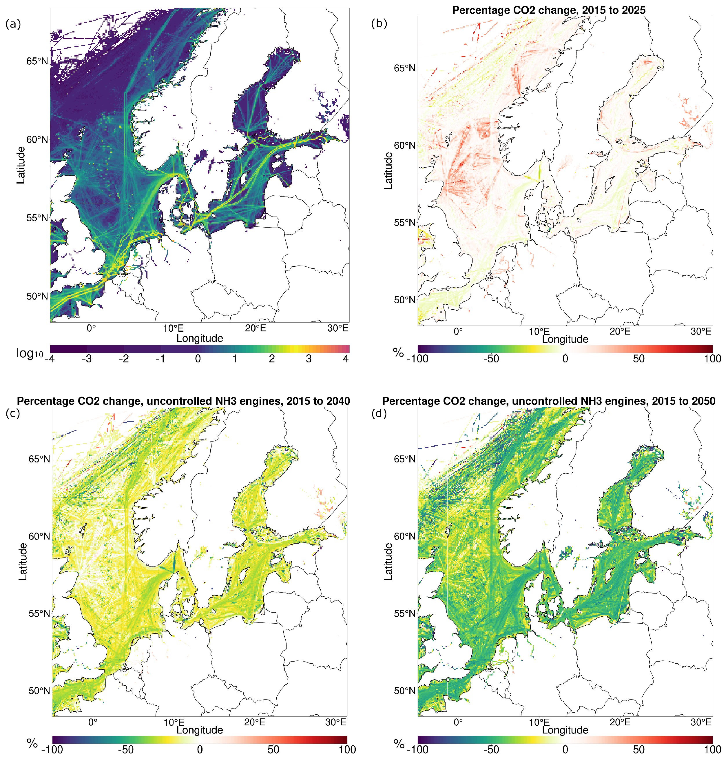
In the following section, the observed emission trends in the created scenarios are explained, starting from the reference year 2015 to the three scenario years 2025, 2040, and 2050. Furthermore, a distinction is made between the “uncontrolled” and “controlled” cases, which refer to the ammonia engine technology used. However, in view of current developments, an application of a technological option similar to the uncontrolled case, but with improvements reducing NO X (to comply with Tier III regulations), N 2 O , and NH 3 emissions, seems most plausible for the year 2050. The technology considered in the controlled case can presumably be expected to emerge temporally after the uncontrolled case [29]. For the uncontrolled case, the evolution of total emission levels for the scenario years considered is shown in Figure 1. For the emission species that differ compared to the controlled case, the developments are shown in Figure 2.
The modeled scenarios assume a broad fuel transition to ammonia by 2050 to meet the decarbonization targets set by the IMO. This transition is planned to proceed via LNG as the main ship fuel used in 2040. Emissions were generally reduced by the IMO’s EEDI measures that required an increasing efficiency of new ship generations built from the beginning of 2013. An offsetting effect to the increased efficiency came from the growing number and size of ships (the latter going hand in hand with higher engine power) to meet the demands of global trade.

3.1. CO2 Emissions

Compared to 2015, CO 2 emissions in the uncontrolled case were modeled to increase by 2% in 2025 and decrease by 18% in 2040 and by 40% in 2050 (Figure 1). In the controlled case, a CO 2 reduction of 47% could be achieved from 2015 to 2050 (Figure 2). The increase in CO 2 emissions by 2025 was based on fleet growth trends by vessel size and number. These trends outweighed the lower CO 2 emissions from LNG-fueled ships (approximately 13% lower CO 2 emissions per gram of fuel, versus residual and distillate fuels), which were increasing in number until 2025 [3]. In the 2040 scenario, a higher percentage of ships used LNG as a bridging technology (57%). In addition, it was assumed that 10% of ships will use ammonia as fuel. In the uncontrolled case, CO 2 emissions from ships using NH 3 as fuel were not zero but reduced by approximately 83%, compared to traditional marine engines powered by fuel oil. In the controlled case, the exhaust gas of the applied ammonia engines is truly carbon-free due to the use of hydrogen as pilot fuel. Both effects together led to a trend reversal and an overall decrease in CO 2 emissions. For the 2050 scenario, 40% of the energy demands in shipping were projected to be met by ammonia, resulting in further reductions in CO 2 emissions.
The designated target of the IMO is a reduction in CO 2 emissions from global shipping by at least 50% in 2050 compared to 2008 [4]. The CO 2 reductions in the uncontrolled case of this study were short by 10 percentage points (40% CO 2 decrease) of achieving the IMO target. In the controlled case, CO 2 reductions were only short by 3 percentage points (47% CO 2 decrease). For achieving a reduction of 50%, differences in CO 2 emissions need to be compensated, e.g., by processes such as Carbon Capture and Storage during fuel production, which were not considered here. Furthermore, this study compares the CO 2 reductions between the years 2050 and 2015. However, results from Kalli et al. [28] suggest that the total CO 2 emissions in the North and Baltic Seas’ Sulfur Emission Control Area (SECA) region varied only a little between the years 2009 and 2015. Thus, a comparison between the years 2050 and 2008 might be similar to the results presented here.
The spatially distributed CO 2 emission fluxes [ g · m 2 · year 1 ] of the reference EI for 2015 on a logarithmic scale are shown in Figure 3a. Figure 3b–d show the percent change in CO 2 emissions for the three future scenarios, compared to the reference EI. In particular, in Figure 3b, the characteristics of the scenario-building method are visible from the differences in percentage CO 2 reductions. In 2025, CO 2 reductions were still small compared to 2015. In some areas, especially in domestic and coastal regions and in the North Sea between Scotland and Norway, no change or even an increase in CO 2 emissions could be observed. These observations could be attributed to fishing vessels and pleasurecrafts as well as vessels whose type could not be determined. All these ships usually sail near the coast, and due to a lack of data, they were not changed in the scenario shipping fleets. A similar observation was made for regions and routes on which mainly newer ships were deployed, as these were not renewed for the 2025 scenario fleet. Nevertheless, in these areas and on these routes, the number of ships was increased and accordingly the emissions compared to 2015. However, overall emissions in these regions were generally low. In 2040 and 2050, a significant decrease in CO 2 is clearly visible along the main shipping routes in the English Channel, along the northern European coastline, and in the Baltic Sea (Figure 3c,d).

3.2. Methane Emissions

Emissions of methane increase by 61% from 2015 to 2025. They peaked in 2040 by an increase of 1105% and were still increased by 631% in 2050, compared to 2015. The reason for this was the increasing number of LNG-fueled ships. LNG-fueled marine engines can leak unburned methane, known as methane slip, which is responsible for the largest part of CH 4 emissions. To effectively reduce the GHG emissions from the shipping sector, this must be carefully considered, as the global warming potential (GWP) of methane is 25 CO 2 equivalents [30] and can outweigh the savings in CO 2 emissions.
This could impede the ambitious GHG reduction targets and demonstrates the need for discerning control that targets methane slip from LNG-fueled ships. Therefore, this topic was included in the list of candidate short-term measures of the IMO’s GHG reduction strategy [4]. In addition, at the COP26 climate summit, more than 100 countries pledged to reduce methane emissions [31].

3.3. N2O Emissions

The third important GHG emitted by ships is nitrous oxide ( N 2 O ). Similar to NO X , nitrous oxide is a byproduct in internal combustion engines that forms from the air that is injected into the cylinders. The use of ammonia as a marine fuel can increase emissions of N 2 O due to additional nitrogen from ammonia combustion. Nitrous oxide is very potent as a greenhouse gas with a GWP of 298 CO 2 equivalents [30]. A 4% increase in N 2 O was projected in the 2025 scenario due to the implemented fleet growth. In the uncontrolled case for the 2040 scenario, a 213% increase in N 2 O emissions was estimated compared to 2015 due to the deployment of the first ammonia-fueled ships (Figure 1). In 2050, a 900% increase was estimated compared to 2015. A reduction in nitrous oxide emissions by a different engine technology or through better control of the combustion process might be possible. This is reflected by the calculations for the controlled case, which projects a reduction in nitrous oxide emissions by 17% in the 2040 scenario and by 29% in 2050 scenario with respect to 2015 (Figure 2).

3.4. CO2 Equivalent Emissions

The effect of the scenario projections on the development of total GHG emissions is illustrated by means of their CO 2 equivalents in Figure 1 and Figure 2. From 2015 to 2025, CO 2 equivalents were modeled to increase by 2%. Compared to 2015, CO 2 equivalents in 2040 were reduced by 9% in the uncontrolled case and 13% in the controlled case. In the 2050 scenario, the reductions were 22% and 44%, respectively. Besides CO 2 , methane and nitrous oxide were considered for the calculation of CO 2 equivalents. An additional consideration of BC with a 100-year GWP of 900 in the calculation of CO 2 equivalents [3] significantly increased the reductions due to a decreased use of fuel oils. In the uncontrolled case, changes in CO 2 equivalent emissions, including BC, were + 0.2 % in 2025, 20 % in 2040, and 31 % in 2050. In the controlled case, these changes were also + 0.2 % in 2025, 24 % in 2040, and 50 % in 2050. These results show the significant differences in overall GHG reductions between the NH 3 engine technologies used. In the controlled scenario for 2050, only 7% of the reduction potential could be attributed to CO 2 without considering the GWP of BC. The major part of 15% could be achieved by a better control of nitrous oxide. A greater reduction potential of 15% was associated with nitrous oxide, which is accessible by a better control of N 2 O emissions. These results suggest not only that CO 2 is important in future legislation that aims at reducing GHG emissions in the shipping sector, but also that emissions of N 2 O need to be included in future regulation measures if a transition towards ammonia as a more climate-friendly fuel is to succeed. The results also highlight the significant contribution of BC to CO 2 equivalent emissions from ships, which can be reduced by transitioning to cleaner and carbon-free fuels.

3.5. NOX Emissions

Nitrogen oxide emissions decreased by 13% in the 2025 scenario compared to 2015 (Figure 1 and Figure 2), primarily due to MARPOL Annex VI NO X control requirements and the implementation of a Nitrogen Emission Control Area (NECA) in the North and Baltic Seas [32,33]. Accordingly, ships that were renewed during the scenario generation had a more recent year of build and thus needed to comply to stricter emission limits. In addition, the higher number of LNG-fueled ships reduced total NO X emissions, as they generally emit less NO X and often even have emissions below the limits of the IMO Tier III Regulation. In 2040, the number of newly built ships that had to comply with the NECA regulations increased. In addition, the share of energy consumed by LNG-fueled vessels increased significantly, by 57%, compared to 2015. For ammonia-fueled ships, the amount of NO X emissions also depends on the technology used and is different for the uncontrolled and controlled cases. Calculations for the uncontrolled case resulted in a NO X emissions decrease by 39% in the 2050 scenario, compared to 2015. Compared to the 2040 scenario, this represented an increase by 41%. It is worth noting that the NO X EFs for the uncontrolled case were about equal to the Tier II limits, although ships built after 2021 are required to comply with the Tier III limits. Therefore, either manufacturers of marine ammonia engines are required to reduce NO X emissions of their products to Tier III standards or ammonia-fueled vessels must be exempted from this regulation in order to operate in the North and Baltic Seas. The NO X EFs for the controlled case were in the magnitude of the Tier III limits. This resulted in a NO X reduction of 62% in the 2040 scenario and of 61% in the 2050 scenario, compared to 2015. In this context, it should be noted that NO X emissions from ammonia-fueled engines could be further reduced through the application of selective catalytic reduction (SCR) or exhaust gas recirculation (EGR) technologies [34].

3.6. Particulate Matter and SO2 Emissions

The reduced use of conventional oil-based fuels in marine engines also led to a reduction in particulate emissions. Particulate matter in ship emissions consists of black carbon (BC), mineral ash (MA), primary organic aerosols (POAs), sulfate ( SO 4 ), and water associated with sulfate ( SO 4 × H 2 O ), which were projected to be reduced by between 73% and 84% in the 2050 uncontrolled scenario (Figure 1). Slightly higher reductions were expected in the controlled case (Figure 2). SO 2 emissions are reduced analogously. In the 2025 scenario, the reductions were mainly based on the shift from distillate fuel (DF) to LNG, since LNG generally produces fewer particles in burning and contains very little sulfur. In the 2025 scenario, the reductions were mainly due to the switch from DF to LNG, which produces fewer particulates when burned. This is also attributable to its lower sulfur content. In the 2040 and 2050 scenarios, particulate emissions were further reduced due to the continued increase in the share of LNG- and NH 3 -fueled ships. In the controlled case, emissions from ammonia combustion could be considered nearly free of primary particulates.

3.7. CO and NMVOC Emissions

Non-methane volatile organic compounds (NMVOCs) and CO emissions increased by 21% and 24%, respectively, in the 2025 scenario compared to 2015 (Figure 1 and Figure 2). The amount of NMVOC emissions from marine diesel engines and LNG-fueled ships is of a comparable magnitude. However, carbon monoxide emissions are higher for LNG-fueled vessels. For this reason, CO emissions increased further for the 2040 scenario, alongside the increasing number of LNG-powered ships. For this reason, CO emissions continued to rise in the 2040 scenario, analogously to the increasing number of LNG-fueled ships. For the uncontrolled and controlled case, NMVOC emissions were at similar levels in the 2040 scenario as in 2015, as additional emissions from fleet growth were offset by the deployment of ammonia-fueled vessels and the EEDI measures (Figure 1 and Figure 2). Since experimentally determined EFs were not available for NMVOC emissions from ammonia engines, they were estimated to be 20% of the NMVOC EFs for marine diesel engines in the uncontrolled case to match the amount of pilot fuel used. In the uncontrolled 2050 scenario, CO emissions increased by 5% and NMVOC emissions decreased by 27% compared to 2015, due to the high number of ships operating on carbon-free ammonia (Figure 1). For the controlled case, a decrease of 3% was modeled for CO and of 35% for NMVOC emissions (Figure 2). The slightly lower emission totals in the controlled case were based on the assumption that ship emissions from ammonia engines are almost free of CO and NMVOCs, which are both carbon compounds.

3.8. Ammonia Emissions

With the introduction of ammonia-powered ships, ammonia slip emerged as a problem. According to Ntziachristos et al., ammonia slip can be up to 8% of the NH 3 consumed for the technology used in the uncontrolled case. Ammonia emissions of 930 Gg were calculated for the uncontrolled 2050 scenario in the regarded domain (Figure 1). This corresponds to approximately twice the ammonia emissions from Germany in 2020, which then amounted to 537 Gg [35]. With the technology of the controlled case, ammonia slip was reduced to approximately 100 ppm , resulting in only 4% of NH 3 emissions, compared to the uncontrolled case. This reduced ammonia emissions to 35 Gg for the controlled 2050 scenario (Figure 2). It should be noted that this ammonia slip, in conjunction with NO X and SO 2 emissions from shipping, is expected to increase concentrations of secondary ammonium aerosols near the shipping lanes, especially in the uncontrolled case. Furthermore, the toxicity of ammonia can be directly harmful to organisms and cause environmental acidification and nitrification [36].

4. Concluding Summary and Outlook

This publication presents a novel methodology for generating ship emission scenarios. The methodology allows simulating physical fleet developments, such as the decommissioning and renewal of ships, fuel type changes, and efficiency gains, implemented through changes to a virtual shipping fleet. Subsequently, the emissions of this fleet can be calculated with the MoSES ship emission model, so that the complex relationships between the energy consumption of several thousand ships and the corresponding emissions can be handled in a computational model. The methodology presented is generally applicable to enable a flexible scenario design, but it is particularly useful for the generation of future scenarios.
One use case for this approach is shown in this work by the creation of three ship emissions inventories for the future scenario years 2025, 2040, and 2050. They cover a domain located in northern Europe that includes the North and Baltic Seas. Motivated by the IMO’s increased efforts to decarbonize the shipping sector and the growing urgency to reduce GHG emissions, the scenarios examine the impact of a broad fuel transition to ammonia in 2050 via LNG as an interim solution in 2040. With respect to the ammonia engine technology, two cases were distinguished. One case assumes a compression ignition engine with marine gas oil as pilot fuel and is referred to as “uncontrolled”, while the other involves a spark ignition engine using hydrogen as the pilot fuel and is referred to as “controlled”. Emission reductions were in general stronger for the controlled case; however, it is assumed that the technology of the uncontrolled case will be more feasible by 2050. In addition, a growing fleet by ship size and number is considered as well as efficiency improvements in accordance with the IMO’s EEDI measures.
Compared to the reference ship emission inventory for 2015, CO 2 emissions decreased by 40% for the uncontrolled 2050 scenario. However, for CO 2 equivalents, the reduction was only 22% (or 31% by including BC in the calculation of CO 2 equivalents). This difference was primarily due to tremendous increases in methane and nitrous oxide emissions, by 613% and 900%, respectively.
NO X emissions were calculated to be reduced by 39% in the uncontrolled 2050 scenario; this includes reductions associated with the implemented NECA regulations in the North and Baltic Seas for fuels other than NH 3 . CO emissions were calculated to increase slightly, by 5%, and NMVOC emissions decreased by 27%. The phasing-out of marine fossil fuels reduced emissions of SO 2 and primary particulate matter from shipping by more than 73%. However, NH 3 slip from ammonia-fueled ships emerged as a new emission species from shipping. For the study region, it amounted to 930 Gg in the uncontrolled 2050 scenario and, in combination with NO X and SO 2 , has the potential to promote the formation of secondary particles near the shipping routes. It should be noted that this slip can be significantly reduced, e.g., by the different technological approach addressed in the controlled case, which reduced ammonia slip to approximately 4%, compared to the uncontrolled case.
To investigate how the projections in these ship emission scenarios affect pollutant concentrations and air quality in the North and Baltic Seas, chemistry transport modeling studies are currently being conducted with the presented ship emission inventories. Future work in the context of ship emission scenarios could address further developments that might be expected in the future. However, the impact of some of these developments is unclear or difficult to quantify at the present time. These include, e.g., politically induced changes in trade relations, which are not considered in the scenarios since the projections in this regard are too uncertain. Furthermore, the scenarios do not take into account a potential non-compliance of ships to cleaner fuels, different engine technologies, or possible new legislation aimed at the mitigation of GHG emissions and/or air pollution. In addition, shore power could play a larger role for berthing ships in the future, which would reduce ship emissions in larger port areas. Moreover, no rerouting of important shipping lanes was considered, e.g., via a possible Arctic route, which may open under ongoing climate change. A newly accessible Arctic route could change the routing of major shipping lanes in the North Sea and even increase shipping traffic. Considering these potential developments, the spatial distribution of ship emissions in the presented inventories should be taken with care. However, we believe that at the regional level, uncertainty in emission factors of future ammonia engines has the most important impact on air quality, and the present calculations provide a good initial quantitative overview of regional ship emissions from ammonia engines, which should be updated as new data become available.

Author Contributions

Conceptualization, D.A.S.; methodology, D.A.S., V.M., R.P., J.H. and L.N.; software, D.A.S.; validation, D.A.S.; formal analysis, D.A.S.; investigation, D.A.S.; resources, V.M.; data curation, D.A.S., J.H., R.P. and L.N.; writing—original draft preparation, D.A.S. and L.N.; writing—review and editing, J.H., M.Q. and V.M.; visualization, D.A.S.; supervision, V.M. and M.Q.; project administration, V.M.; funding acquisition, V.M. and M.Q. All authors have read and agreed to the published version of the manuscript.

Funding

This research and APC were funded by the German Federal Maritime and Hydrographic Agency (BSH) in the framework of the “SeAir” project (BSH contract code: 10042629, Hereon contract code: 430/2018) and the EU Horizon 2020 project “SCIPPER” (No. 814893).

Institutional Review Board Statement

Not applicable.

Informed Consent Statement

Not applicable.

Data Availability Statement

The data presented in this study are available on request from the corresponding author.

Conflicts of Interest

The authors declare no conflict of interest.

Abbreviations

The following abbreviations are used in this manuscript:
AISAutomatic Identification System
BCBlack Carbon
BSHGerman Federal Maritime and Hydrographic Agency
CO2eqCarbon Dioxide Equivalents
COP2626th United Nations Climate Change Conference of the Parties
DFDistillate Fuel
DNV-GLDet Norkse Veritas-Germanischer Lloyd
EEDIEnergy Efficiency Design Index
EFEmission Factor
EGRExhaust Gas Recirculation
EIEmission Inventory
EMSAEuropean Maritime Safety Agency
GHGGreenhouse Gas
GWPGlobal Warming Potential
IHSInformation Handling Services
IMOInternational Maritime Organization
LNGLiquiefied Natural Gas
MAMineral Ash
MARPOLInternational Convention for the Prevention of Pollution from Ships
MeOHMethanol
MEPCMarine Environmental Protection Committee
MGOMarine Gas Oil
MoSESModular Ship Emission modeling System
NECANitrogen Emission Control Area
NMVOCNon-methan Volatile Organic Compounds
NO X Nitrogen Oxide
PMParticulate Matter
POAPrimary Organic Aerosols
SCRSelective Catalytic Reduction
SECASulfur Emission Control Area
SISpark Ignition
SO X Sulfur Oxide
UNCTADUnited Nations Conference on Trade and Development

Appendix A. Emission Factors

Table A1. Emission factors in [ g / kWh ] used for the calculation of the reference and scenario ship emission inventories. NH 3 unc. refers to the case implementing the uncontrolled ammonia engine technology, NH 3 con. to the controlled technology. LNG refers to ships fueled with liquefied natural gas, MeOH refers to ships fueled with methanol, DF refers to ships fueled with marine diesel oil, and RF refers to ships fueled with marine residual fuels. S F C is the specific fuel consumption [ g / kWh ] , E L is the ship engine load, and F S C is the fuel sulfur content as mass fraction. The descriptors “Main” and “Aux” refer to emission factors applied to the main or auxiliary engine of a ship, respectively.
Emission SpeciesNH3 Unc.NH3 Con.LNGMeOHDFRF
BC 00 0.003  a 3.49 × 10 5 × e 0.056 E L + 1.61 × 10 5  a x × c o r r B C x ( Main DF ) = 0.03 ,
x ( Main RF ) = 0.06 , x ( Aux DF , RF ) = 0.15  b
CH 4 00Main: 0.2 ,
Aux: 5.5  a
0.013 × E L + 0.03  c 0.01  a 0.01  a
CO 0.09  d0 1.04  a 5 E L + 3 E L 2 13 E L + 10  c 0.44 0.54  b,e 0.54  a
CO 2 110 d0 2.75 × S F C  a 1.375 × S F C  a 3.206 × S F C  a 3.114 × S F C  a
MA 0000 F S C × 0.02 × S F C  f
N 2 O 0.778  d 0.015  d 0.03  a 0.003  a 0.03 0.034  b,e 0.03 0.034  b,e
NH 3 31.2  d 1.17  d0000
NO X 10 da,g 1.3  a 9 E L 2 20 E L + 20  cIMO Tier III limits h
NMVOC 00 0.5  a 0.053 0.063  b,d 0.1 1.8  d,i
POA 0000 0.2 × c o r r P O A ; if E L < 0.15 : c o r r = 3.3 , else:
c o r r P O A = 1.024 / ( 1 47.660 × e 32.547 × E L )  a
SO 2 0.065  d0 3.17 × 10 5 × S F C  a 0.00264 × S F C  a S F C × F S C × 1.998 × 0.97753  f
SO 4 0.0013  j000 S F C × F S C × ( 0.01 + E L × x ) × 2.996 ;
x ( D F ) = 0.004 , x ( R F ) = 0.035 f
a: 4. IMO GHGS [3]. b: Several correction functions (corr) increase BC emissions for different lower loads and can be found in the original manuscript by Aulinger et al., 2016 [37]. c: Fridell et al., 2021 [38]. d: Ntziachristos et al., 2021 (personal communication). e: Engine RPM-dependent. f: Schwarzkopf et al., 2021 [15]. g: This EF considers the application of selective catalytic reduction (SCR) or exhaust gas recirculation (EGR). h: For ships built in 2021 or later (see IMO NECA [21,22]; otherwise, see [15,39]). i: Dependent on ship engine load and navigational status. For details, see EMEP 2019 [40]. j: For this EF, 2% of SO2 emissions mass is assumed.

References

  1. UNCTAD. Review of Maritime Transport 2019; Technical Report; United Nations Conference on Trade and Development, United Nations Publications: New York, NY, USA, 2020; p. 89. [Google Scholar]
  2. Fridell, E. Emissions and Fuel Use in the Shipping Sector; Elsevier Inc.: Amsterdam, The Netherlands, 2018; pp. 19–33. [Google Scholar] [CrossRef]
  3. IMO. Fourth IMO GHG Study; Technical Report; International Maritime Organization: London, UK, 2021. [Google Scholar]
  4. IMO MEPC. Initial IMO Strategy on Reduction of GHG Emission from Ships. Resolution MEPC.304(72) (Adopted on 13 April 2018); Technical Report April; International Maritime Organization: London, UK, 2018. [Google Scholar]
  5. IMO. MEPC.203(62); Technical Report July; International Maritime Organization: London, UK, 2011. [Google Scholar]
  6. ITF/OECD. Decarbonising Maritime Transport. Pathways to Zero-Carbon Shipping by 2035; Technical Report; International Transport Forum, OECD Publishing: Paris, France, 2018. [Google Scholar]
  7. Balcombe, P.; Brierley, J.; Lewis, C.; Skatvedt, L.; Speirs, J.; Hawkes, A.; Staffell, I. How to decarbonise international shipping: Options for fuels, technologies and policies. Energy Convers. Manag. 2019, 182, 72–88. [Google Scholar] [CrossRef]
  8. Shih, Y.C.; Tzeng, Y.A.; Cheng, C.W.; Huang, C.H. Speed and Fuel Ratio Optimization for a Dual-Fuel Ship to Minimize Its Carbon Emissions and Cost. J. Mar. Sci. Eng. 2023, 11, 758. [Google Scholar] [CrossRef]
  9. Wang, X.T.; Liu, H.; Lv, Z.F.; Deng, F.Y.; Xu, H.L.; Qi, L.J.; Shi, M.S.; Zhao, J.C.; Zheng, S.X.; Man, H.Y.; et al. Trade-linked shipping CO2 emissions. Nat. Clim. Chang. 2021, 11, 945–951. [Google Scholar] [CrossRef]
  10. Hansson, J.; Brynolf, S.; Fridell, E.; Lehtveer, M. The potential role of ammonia as marine fuel-based on energy systems modeling and multi-criteria decision analysis. Sustainability 2020, 12, 3265. [Google Scholar] [CrossRef]
  11. Cheliotis, M.; Boulougouris, E.; Trivyza, N.L.; Theotokatos, G.; Livanos, G.; Mantalos, G.; Stubos, A.; Stamatakis, E.; Venetsanos, A. Review on the safe use of ammonia fuel cells in the maritime industry. Energies 2021, 14, 3023. [Google Scholar] [CrossRef]
  12. Dolan, R.H.; Anderson, J.E.; Wallington, T.J. Outlook for ammonia as a sustainable transportation fuel. Sustain. Energy Fuels 2021, 5, 4830–4841. [Google Scholar] [CrossRef]
  13. Wang, Y.; Cao, Q.; Liu, L.; Wu, Y.; Liu, H.; Gu, Z.; Zhu, C. A review of low and zero carbon fuel technologies: Achieving ship carbon reduction targets. Sustain. Energy Technol. Assess. 2022, 54, 102762. [Google Scholar] [CrossRef]
  14. Perčić, M.; Vladimir, N.; Jovanović, I.; Koričan, M. Application of fuel cells with zero-carbon fuels in short-sea shipping. Appl. Energy 2022, 309, 118463. [Google Scholar] [CrossRef]
  15. Schwarzkopf, D.A.; Petrik, R.; Matthias, V.; Quante, M.; Majamäki, E.; Jalkanen, J.P. A ship emission modeling system with scenario capabilities. Atmos. Environ. X 2021, 12, 100132. [Google Scholar] [CrossRef]
  16. DNV-GL. Maritime Forecast to 2050, 2020th ed.; Technical Report; DNV-GL—Maritime: Bærum, Norway, 2020. [Google Scholar]
  17. Jalkanen, J.P.; Brink, A.; Kalli, J.; Pettersson, H.; Kukkonen, J.; Stipa, T. A modelling system for the exhaust emissions of marine traffic and its application in the Baltic Sea area. Atmos. Chem. Phys. 2009, 9, 9209–9223. [Google Scholar] [CrossRef]
  18. Jalkanen, J.P.; Johansson, L.; Kukkonen, J.; Brink, A.; Kalli, J.; Stipa, T. Extension of an assessment model of ship traffic exhaust emissions for particulate matter and carbon monoxide. Atmos. Chem. Phys. 2012, 12, 2641–2659. [Google Scholar] [CrossRef]
  19. Johansson, L.; Jalkanen, J.p.; Kukkonen, J. Global assessment of shipping emissions in 2015 on a high spatial and temporal resolution. Atmos. Environ. 2017, 167, 403–415. [Google Scholar] [CrossRef]
  20. Winnes, H.; Fridell, E.; Yaramenka, K.; Nelissen, D.; Faber, J.; Ahdour, S. NOx Controls for Shipping in EU Seas; Technical Report June; Transport & Environment, IVL: Stockholm, Sweden, 2016. [Google Scholar]
  21. IMO MEPC. Resolution MEPC.177(58); Technical Report; International Maritime Organization: London, UK, 2008. [Google Scholar]
  22. IMO MEPC. RESOLUTION MEPC.251(66); Technical Report; International Maritime Organization: London, UK, 2014. [Google Scholar]
  23. Fridell, E.; Parsmo, R.; Boteler, B.; Troeltzsch, J.; Kowalczyk, U.; Piotrowicz, J.; Jalkanen, J.P.; Johansson, L.; Matthias, V.; Ytreberg, E. Sustainable Shipping and Environment of the Baltic Sea Region (SHEBA) Deliverable 1.4, Type RE; Technical Report; IVL: Stockholm, Sweden, 2016; Available online: https://www.sheba-project.eu/imperia/md/content/sheba/deliverables/sheba_d1.4_final.pdf (accessed on 17 February 2023).
  24. Ushakov, S.; Stenersen, D.; Einang, P.M. Methane slip from gas fuelled ships: A comprehensive summary based on measurement data. J. Mar. Sci. Technol. 2019, 24, 1308–1325. [Google Scholar] [CrossRef]
  25. Yousefi, A.; Guo, H.; Dev, S.; Lafrance, S.; Liko, B. A study on split diesel injection on thermal efficiency and emissions of an ammonia/diesel dual-fuel engine. Fuel 2022, 316, 123412. [Google Scholar] [CrossRef]
  26. Wu, X.; Feng, Y.; Gao, Y.; Xia, C.; Zhu, Y.; Shreka, M.; Ming, P. Numerical simulation of lean premixed combustion characteristics and emissions of natural gas-ammonia dual-fuel marine engine with the pre-chamber ignition system. Fuel 2023, 343, 127990. [Google Scholar] [CrossRef]
  27. Westlye, F.R.; Ivarsson, A.; Schramm, J. Experimental investigation of nitrogen based emissions from an ammonia fueled SI-engine. Fuel 2013, 111, 239–247. [Google Scholar] [CrossRef]
  28. Kalli, J.; Jalkanen, J.P.; Johansson, L.; Repka, S. Atmospheric emissions of European SECA shipping: Long-term projections. WMU J. Marit. Aff. 2013, 12, 129–145. [Google Scholar] [CrossRef]
  29. de Vries, N. Safe and Effective Application of Ammonia as a Marine Fuel. Master’s Thesis, Delft University of Technology, Delft, The Netherlands, 2019. [Google Scholar]
  30. Forster, P.; Ramaswamy, V.; Artaxo, P.; Berntsen, T.; Betts, R.; Fahey, D.; Haywood, J.; Lean, J.; Lowe, D.; Myhre, G.; et al. Changes in Atmospheric Constituents and in Radiative Forcing; Technical Report; IPCC: Cambridge, UK; New York, NY, USA, 2007. [Google Scholar] [CrossRef]
  31. EU Statement. Launch by United States, the European Union, and Partners of the Global Methane Pledge to Keep 1.5 °C within Reach. 2021. Available online: https://ec.europa.eu/commission/presscorner/detail/en/statement_21_5766 (accessed on 27 April 2022).
  32. MEPC, I. Resolution MEPC.75(40) Protocol to the MARPOL Convention with Added Annex VI; Technical Report; International Maritime Organization: London, UK, 1997. [Google Scholar]
  33. IMO MEPC. MEPC 70/INF.34; Technical Report; International Maritime Organization: London, UK, 2016. [Google Scholar]
  34. Mounaïm-Rousselle, C.; Brequigny, P. Ammonia as Fuel for Low-Carbon Spark-Ignition Engines of Tomorrow’s Passenger Cars. Front. Mech. Eng. 2020, 6, 70. [Google Scholar] [CrossRef]
  35. Umweltbundesamt (German Environment Agency). Ammoniak-Emissionen (Ammonia Emissions). 2020. Available online: https://www.umweltbundesamt.de/daten/luft/luftschadstoff-emissionen-in-deutschland/ammoniak-emissionen#entwicklung-seit-1990 (accessed on 16 February 2022).
  36. Asman, W.A.; Sutton, M.A.; Schjørring, J.K. Ammonia: Emission, atmospheric transport and deposition. New Phytol. 1998, 139, 27–48. [Google Scholar] [CrossRef]
  37. Aulinger, A.; Matthias, V.; Zeretzke, M.; Bieser, J.; Quante, M.; Backes, A. The impact of shipping emissions on air pollution in the Greater North Sea region—Part 1: Current emissions and concentrations. Atmos. Chem. Phys. Discuss. 2016, 15, 11277–11323. [Google Scholar] [CrossRef]
  38. Fridell, E.; Salberg, H.; Salo, K. Measurements of Emissions to Air from a Marine Engine Fueled by Methanol. J. Mar. Sci. Appl. 2021, 20, 138–143. [Google Scholar] [CrossRef]
  39. Zeretzke, M. Entwicklung eines Modells zur Quantifizierung von Luftschadstoffen, die Durch Schiffsdieselmotoren auf See Emittiert Werden. Master’s Thesis, Technische Universität Hamburg Harburg, Hamburg, Germany, 2013. [Google Scholar]
  40. EMEP/EEA. EMEP/EEA Air Pollutant Emission Inventory Guidebook 2019; European Environment Agency: Copenhagen, Denmark, 2019. [Google Scholar] [CrossRef]
Figure 1. Development of total annual emissions from 2015 to 2050 in the North and Baltic Sea domain (see Figure 3 for the spatial extent of the domain). For NH 3 -powered engines, a compression ignition engine with marine diesel oil as pilot fuel is considered, which is referred to as the “uncontrolled” case. Annual emission totals are listed without brackets above their corresponding bars. Values for CO 2 were divided by 500, for NH 3 by 5, for NO X by 10, and for CO 2 equivalents by 500 to fit the scale. The values resulting from this division are given in brackets above their corresponding bars.
Atmosphere 14 00879 g001
Figure 2. Development of total annual emissions from 2015 to 2050 in the North and Baltic Sea domain (see Figure 3 for the spatial extent of the domain). For NH 3 -powered engines, a spark ignition engine with hydrogen as pilot fuel is considered, which is referred to as the “controlled” case. The figure shows only emission species whose development is different in the controlled case than in the uncontrolled case. Annual emission totals are listed without brackets above their corresponding bars. Values for CO 2 were divided by 500, for NH 3 by 10, for NO X by 10, and for CO 2 equivalents by 500 to fit the scale. The values resulting from this division are given in brackets above their corresponding bars.
Atmosphere 14 00879 g002
Figure 3. CO 2 emission fluxes in [ g · m 2 · year 1 ] from the reference emission inventory (2015, (a)) and the percentage change from the scenario emission inventories for the years 2025 (b), 2040 (c), and 2050 (d), compared to the reference.
Atmosphere 14 00879 g003
Table 1. Increase in number of ships and capacity increase in percent for all three scenarios, based on Fridell et al. [23]. Annual efficiency increases based on IMO Energy Efficiency Design Index and average ship lifetimes from Winnes et al. [20] for the ship types considered.
Ship Number Incr. [%]Capacity Incr. (crel) [%]Eff. Incr. [%]Lifetime [y]
Ship Type/Year202520402050202520402050Annual
Bulk2 5.1 7.2 5.1 12.5 19.1 0.99 19
Cargo  a 8.3 22.2 32.7 10.9 26.9 37.9 0.82 26
Cruise 10.5 28.2 41.6 4.6 9.9 12.2 0.74 27
Passenger 12.1 30.8 43.1 13.8 35.4 48.1 0.69 27
Tanker 12.7 34.7 51.8 22.5 64.9 101.0 0.73 26
Other 4.6 9.9 12.2 4.6 9.9 12.2 0.69 25
a For the ship type Cargo, the sum for container and general cargo ships was used, weighted by the ship type distribution, according to the UNCTAD Report 2020.
Table 2. Percentage of energy consumption by fuel type for the reference emissions inventory (2015) and the three scenarios created (2025, 2040, 2050), according to DNV-GL [16].
Fuel Type/Year2015202520402050
Residual fuel 14.97 12.75 101
Distillate fuel 83.93 73.75 2223
LNG 1.19 13.5 5733
MeOH 0.05 012
NH 3 001040
Disclaimer/Publisher’s Note: The statements, opinions and data contained in all publications are solely those of the individual author(s) and contributor(s) and not of MDPI and/or the editor(s). MDPI and/or the editor(s) disclaim responsibility for any injury to people or property resulting from any ideas, methods, instructions or products referred to in the content.

