
A Hurricane Initialization Scheme with 4DEnVAR Satellite Ozone and Bogus Data Assimilation (SOBDA) and Its Application: Case Study

Abstract
:1. Introduction
2. Data and Methodology
2.1. AIRS Ozone Data and Bogus Data
2.2. Numerical Model and Observation Operator
2.3. 4DEnVar Method
3. Case Description and Experiment Design
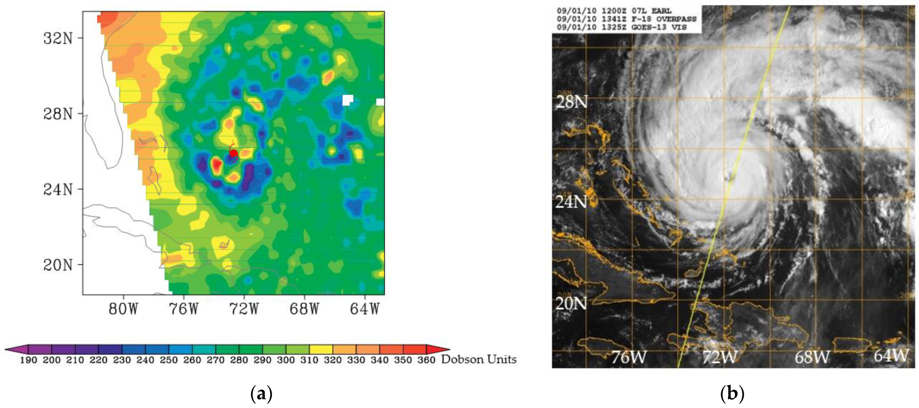
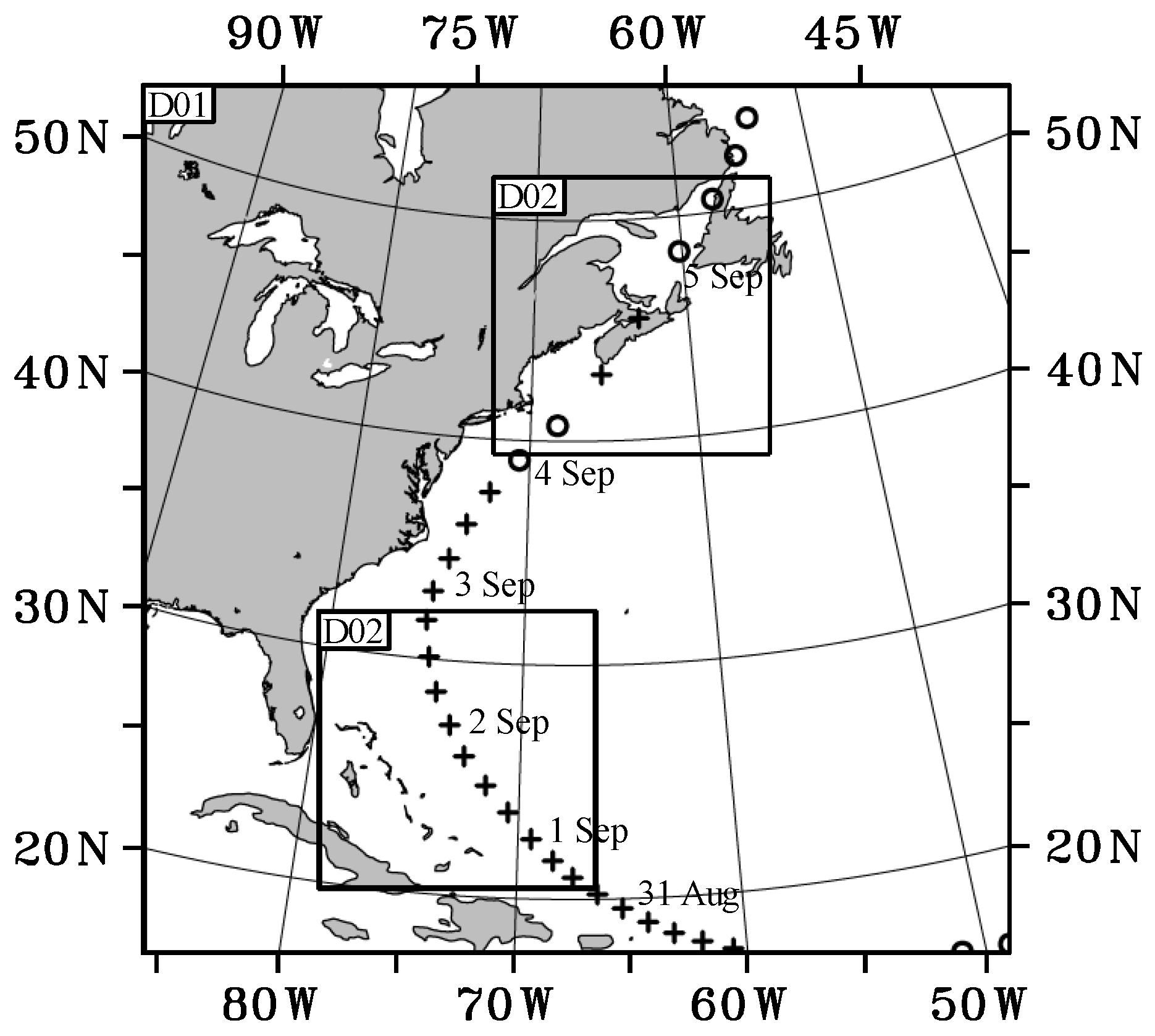
3.1. Case Description
3.2. Experiment Design
4. Numerical Results
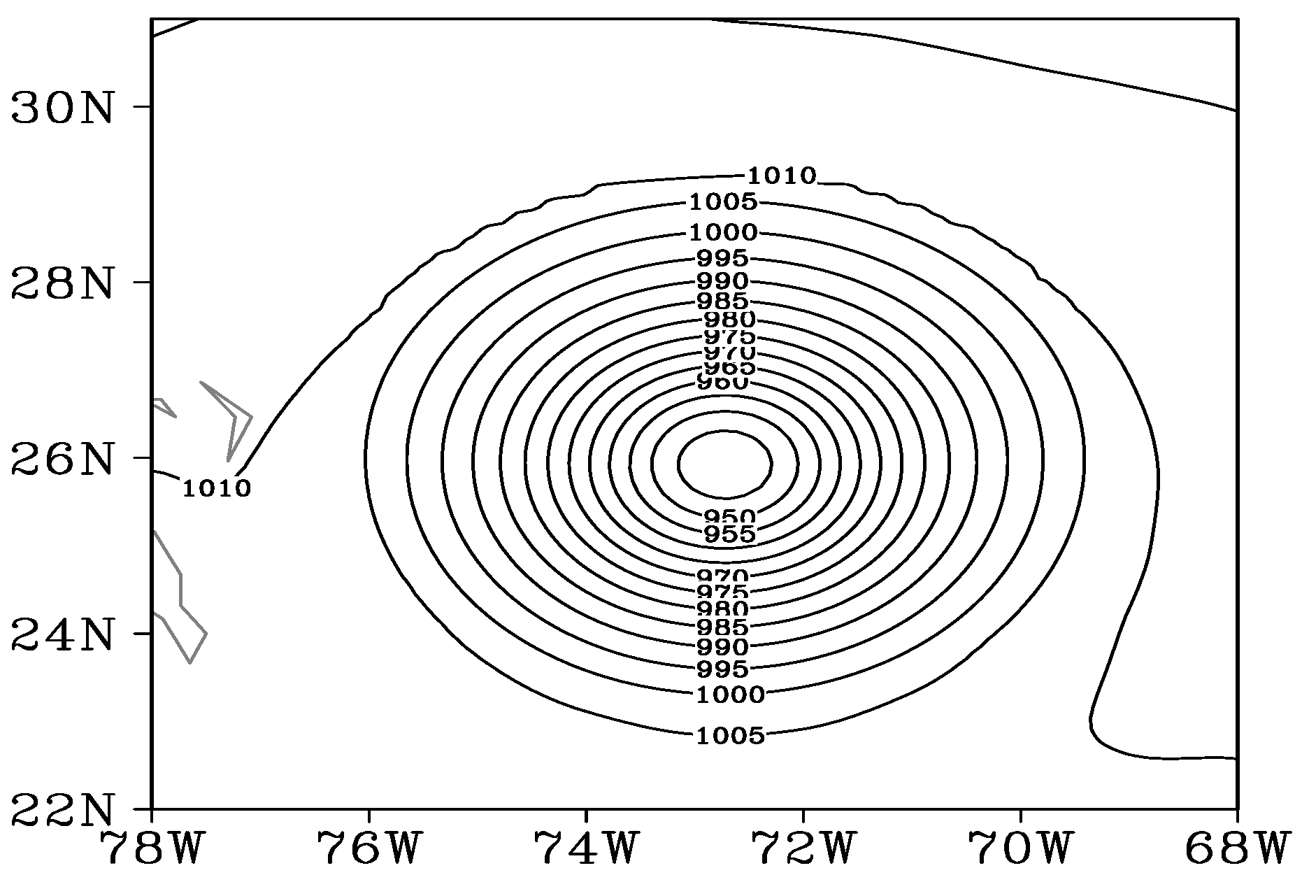
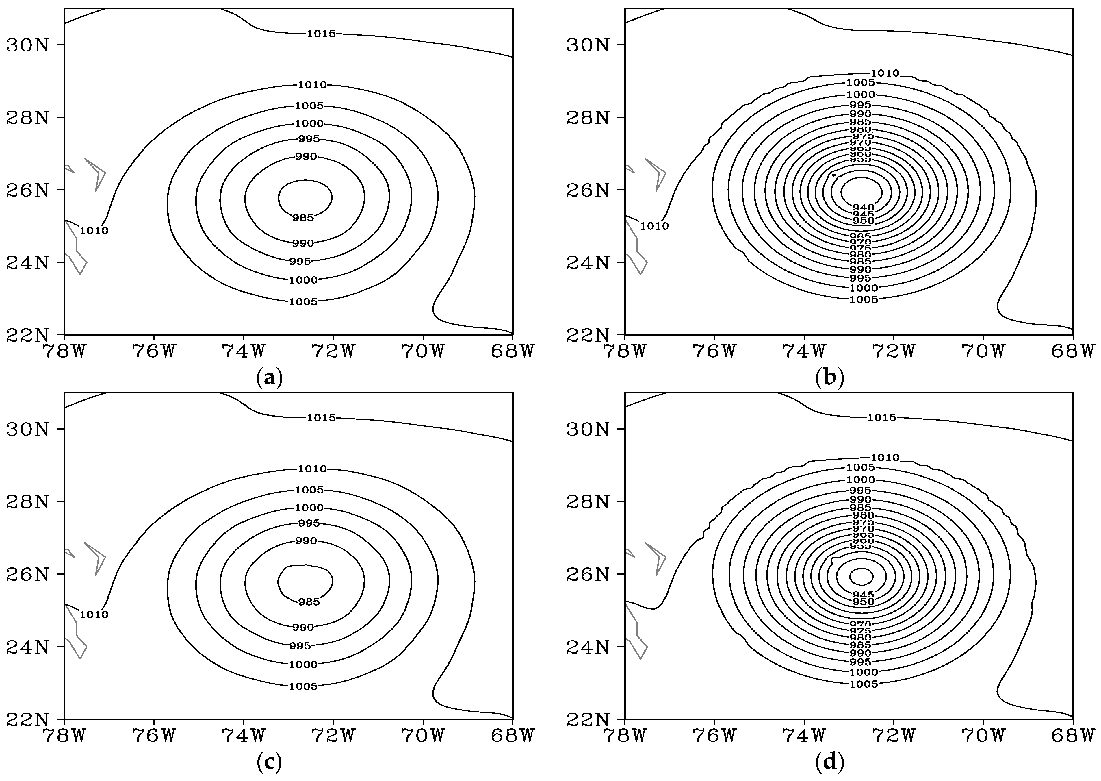
4.1. Initial Structure
4.2. Track and Intensity
4.3. Causes of Simulated Differences
4.4. Impacts of Ensemble Size
5. Summary
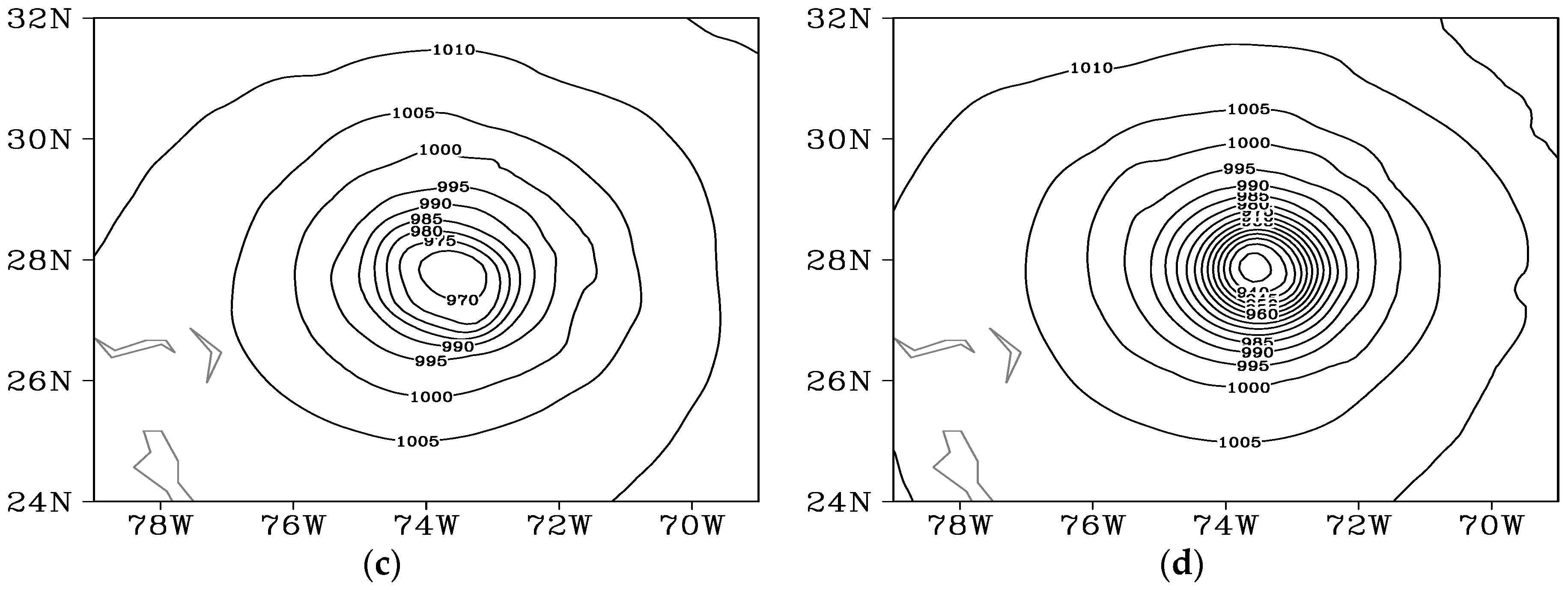
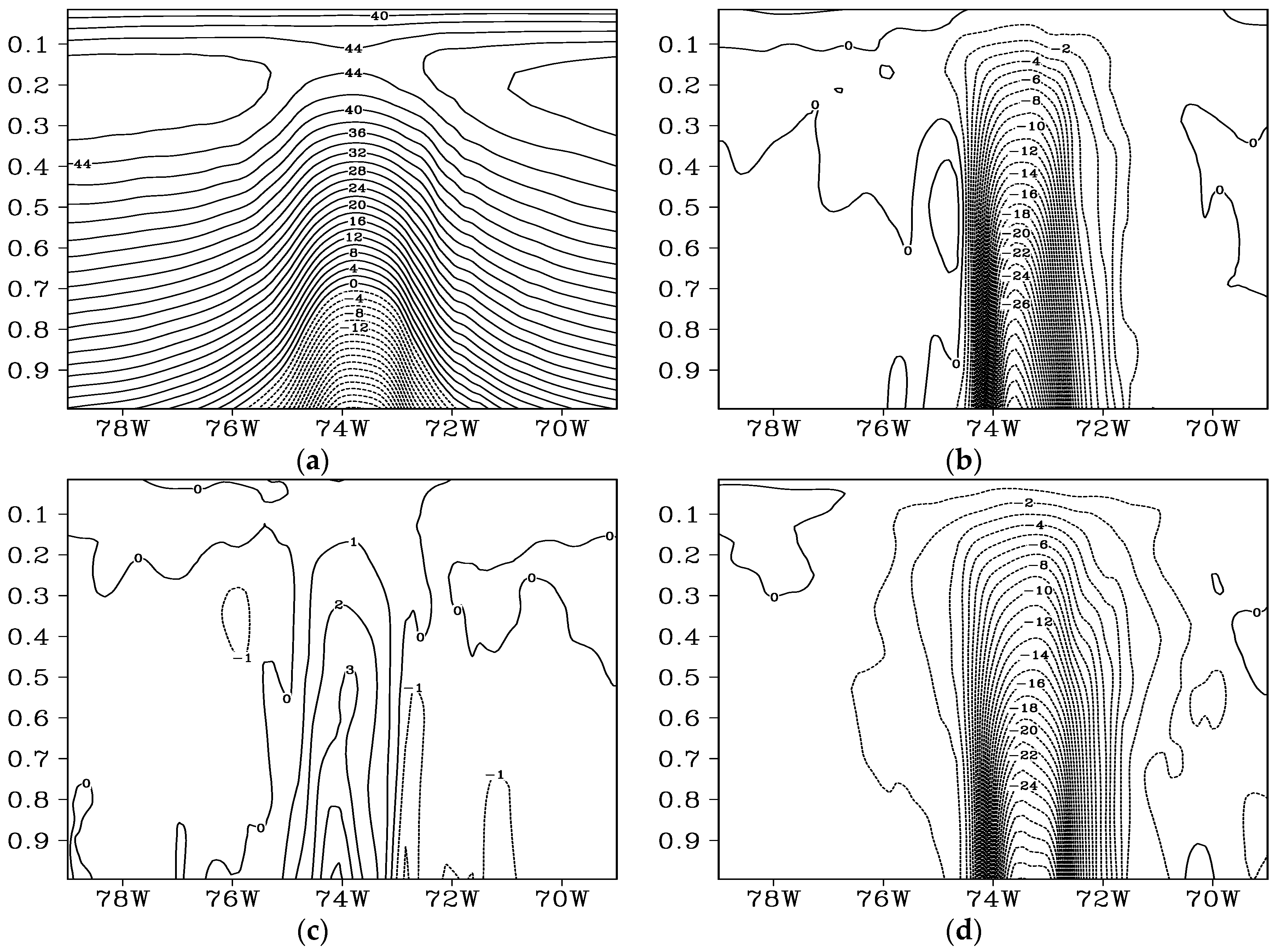
- (1)
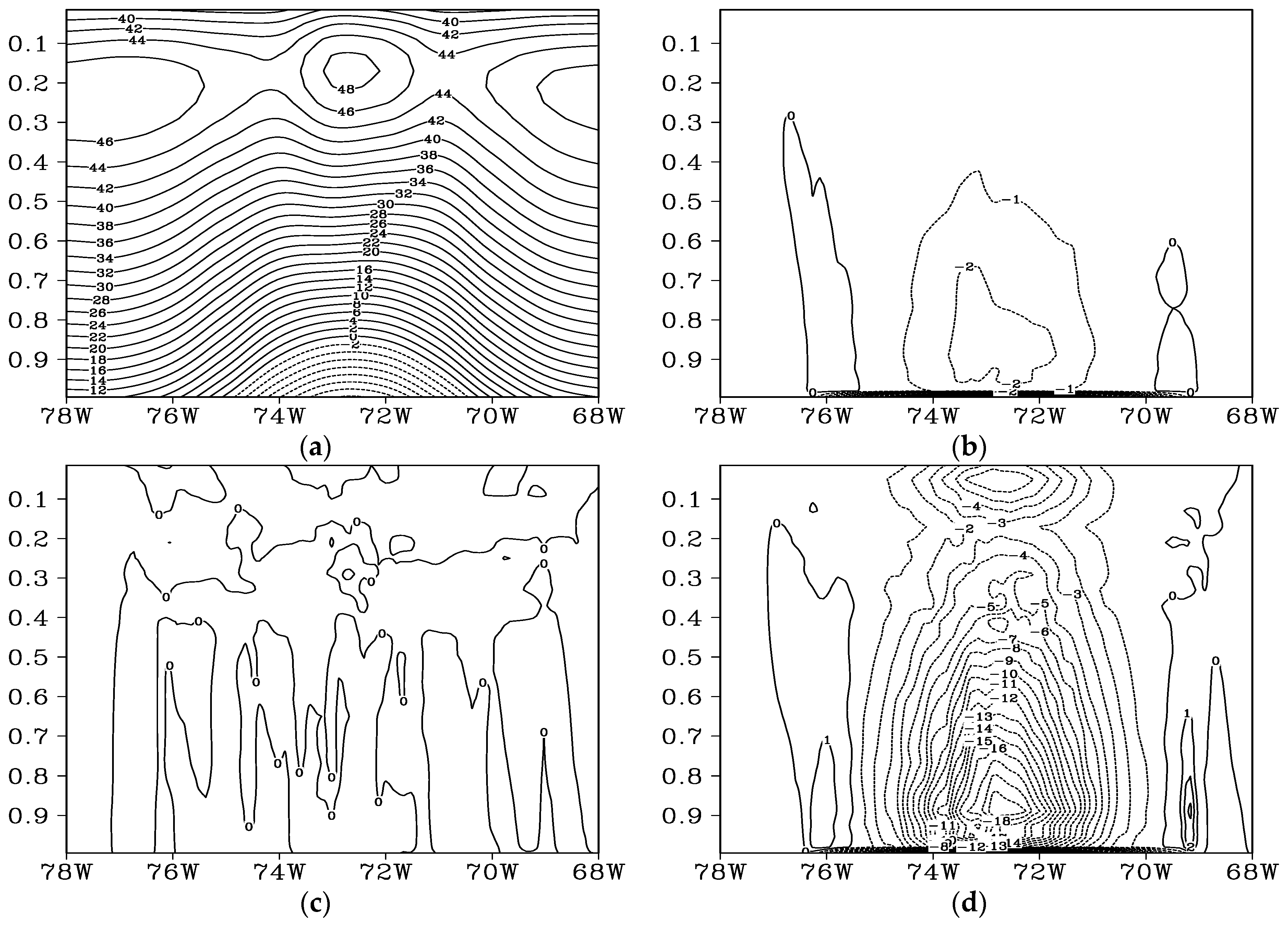
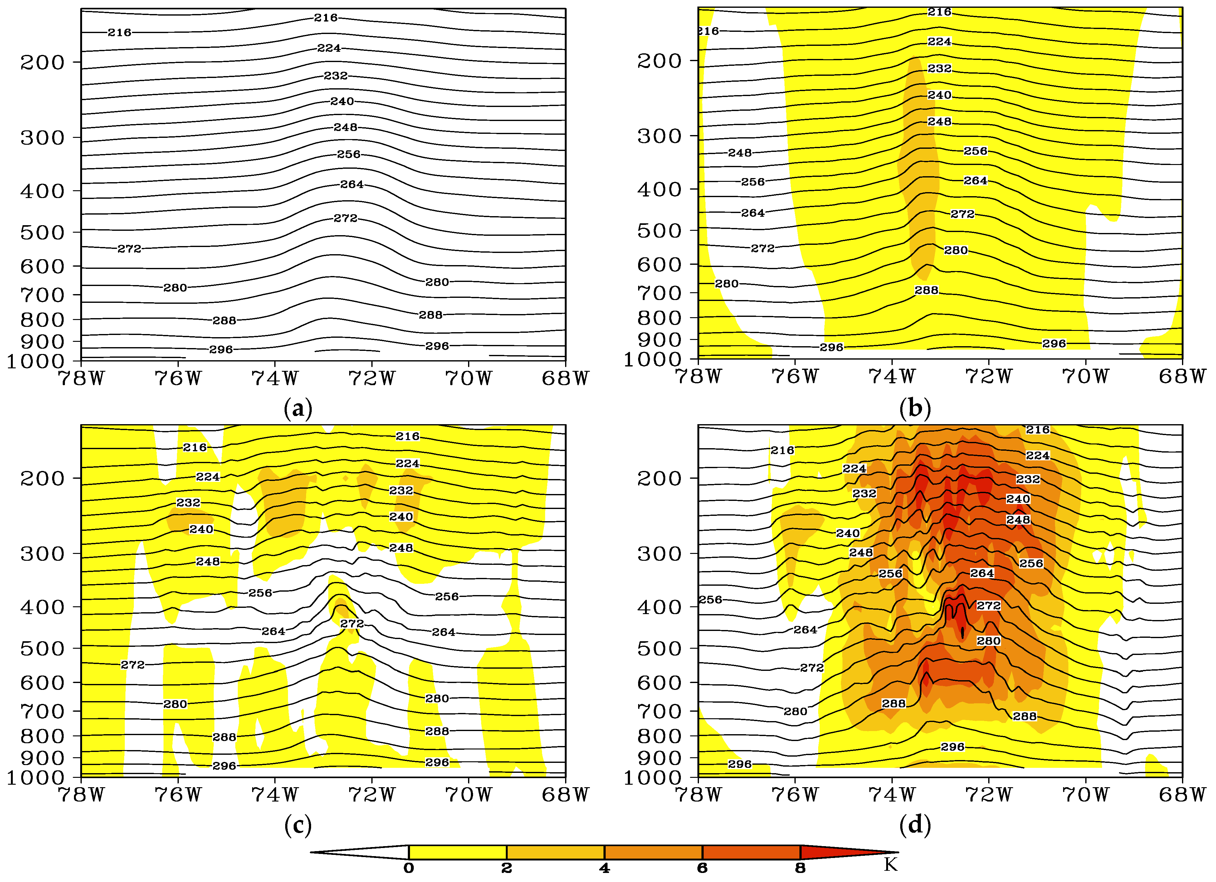
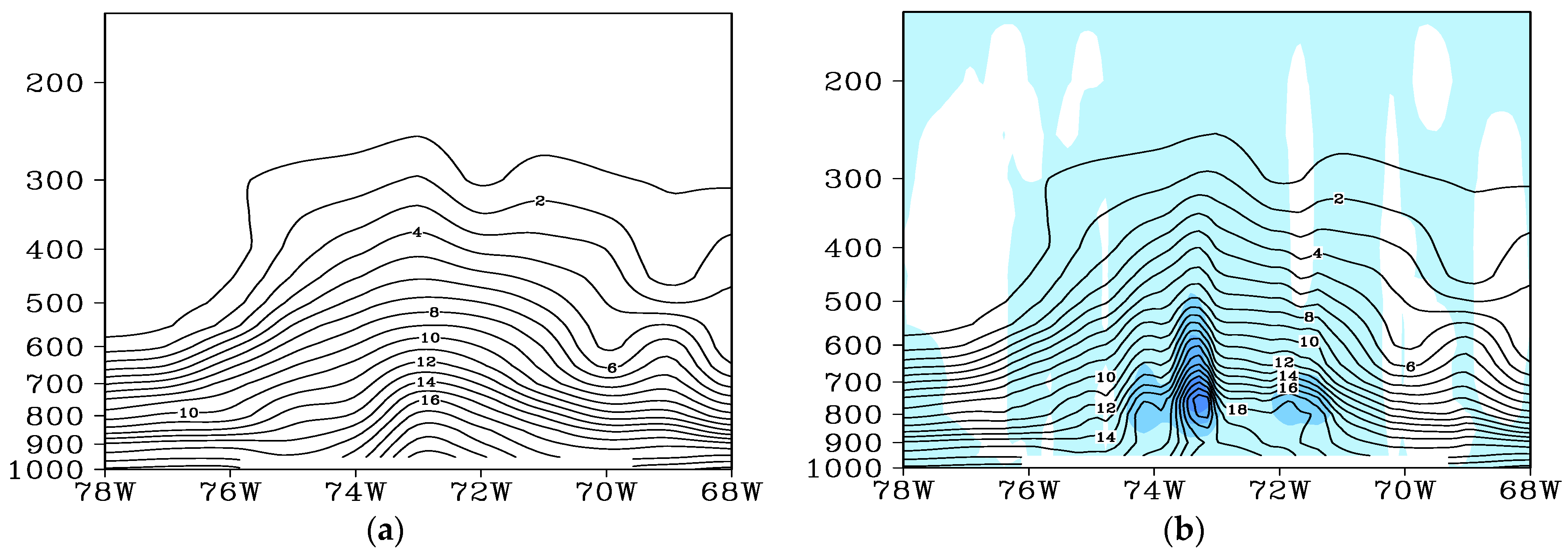
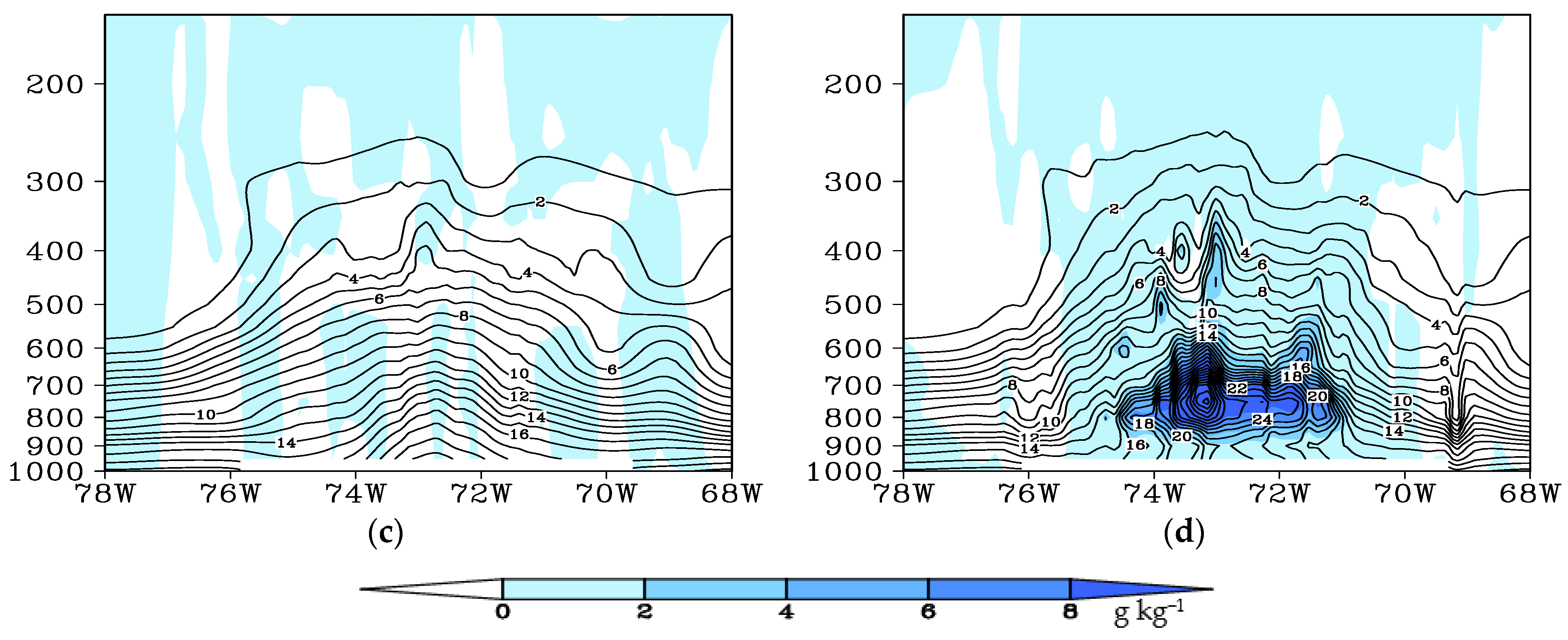
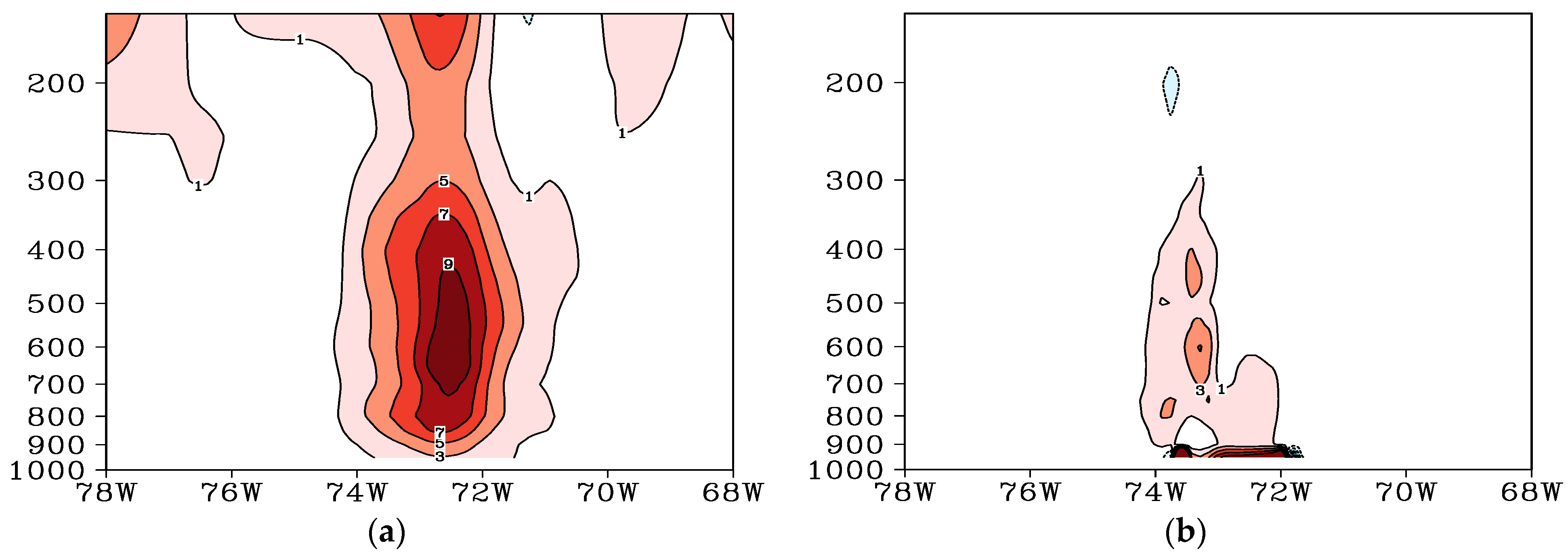
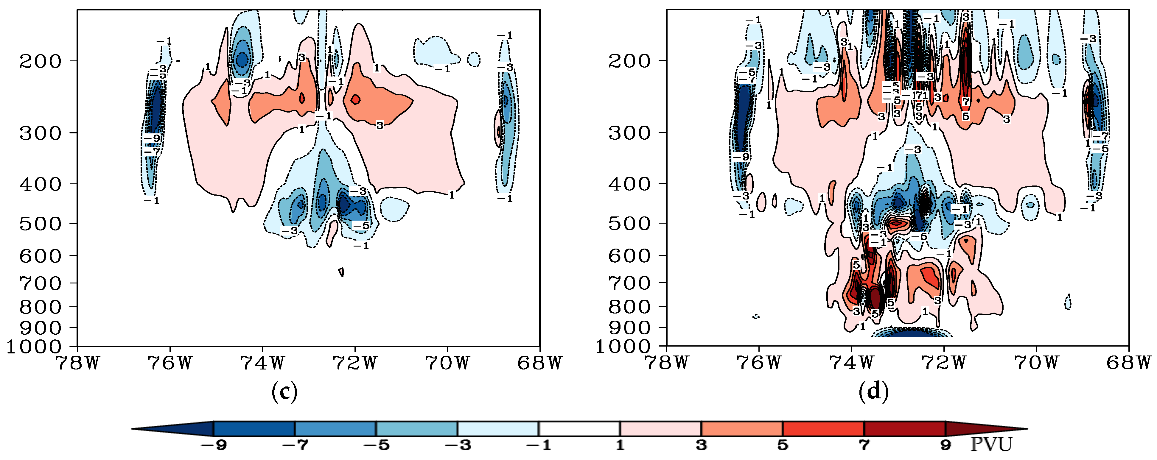
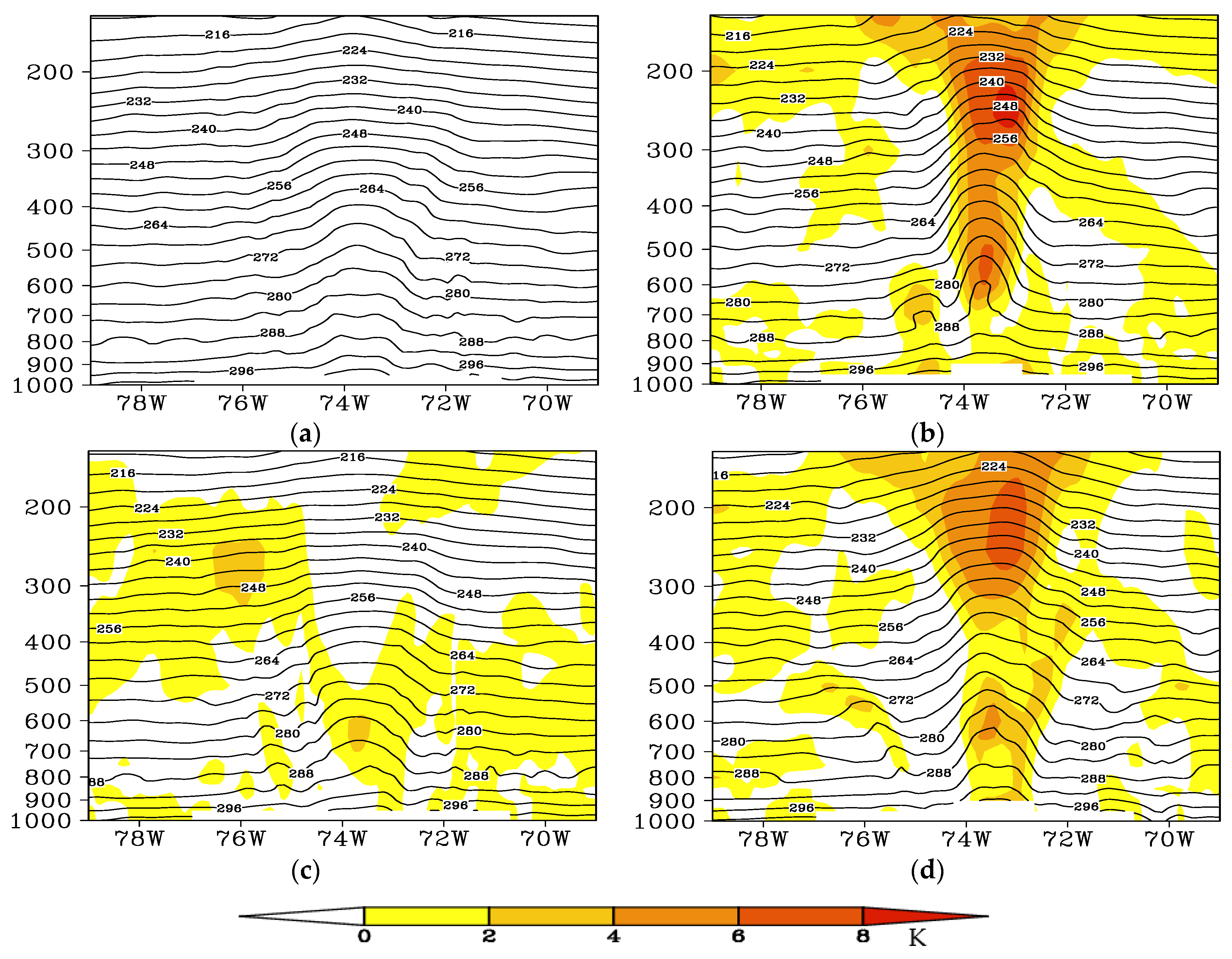
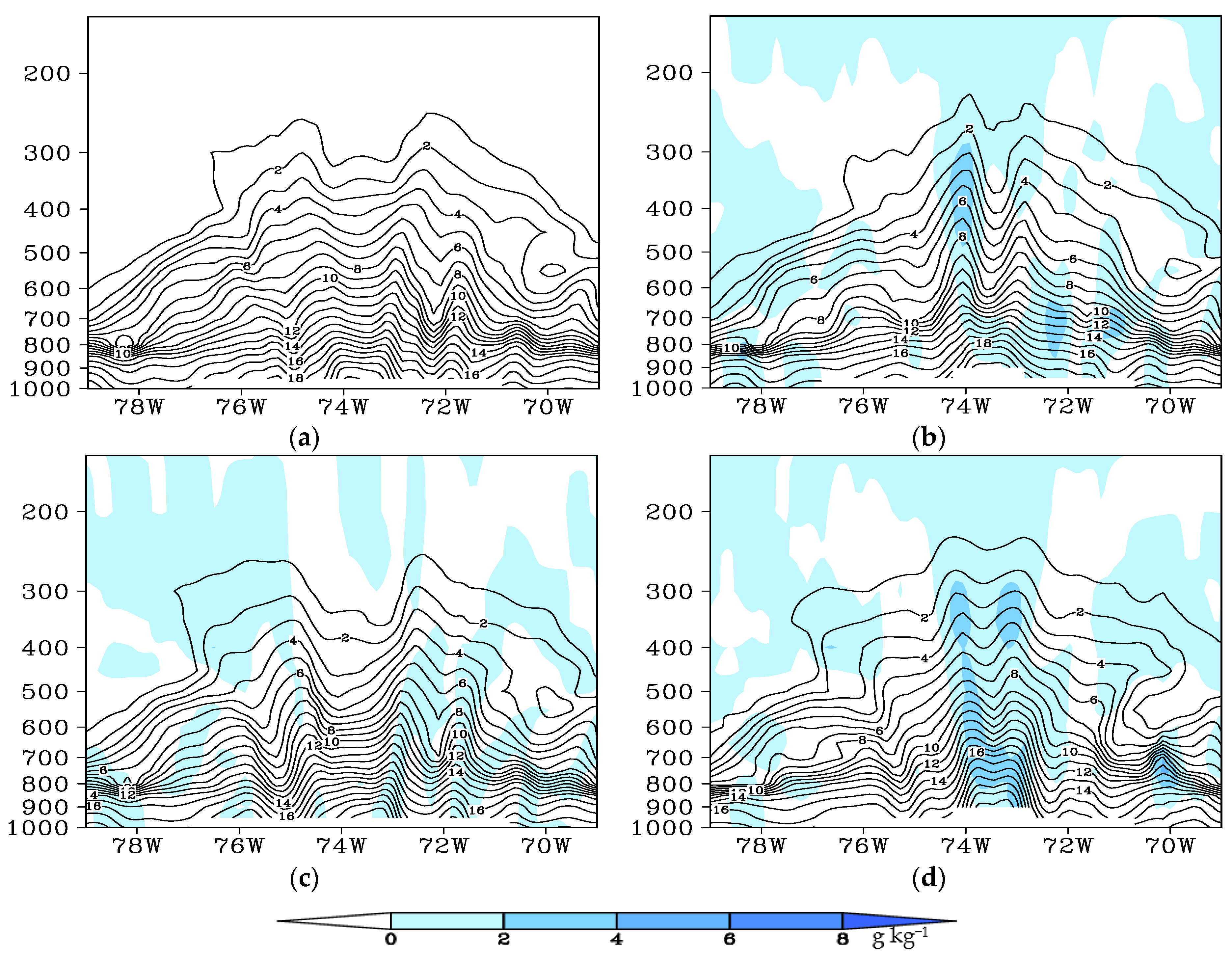
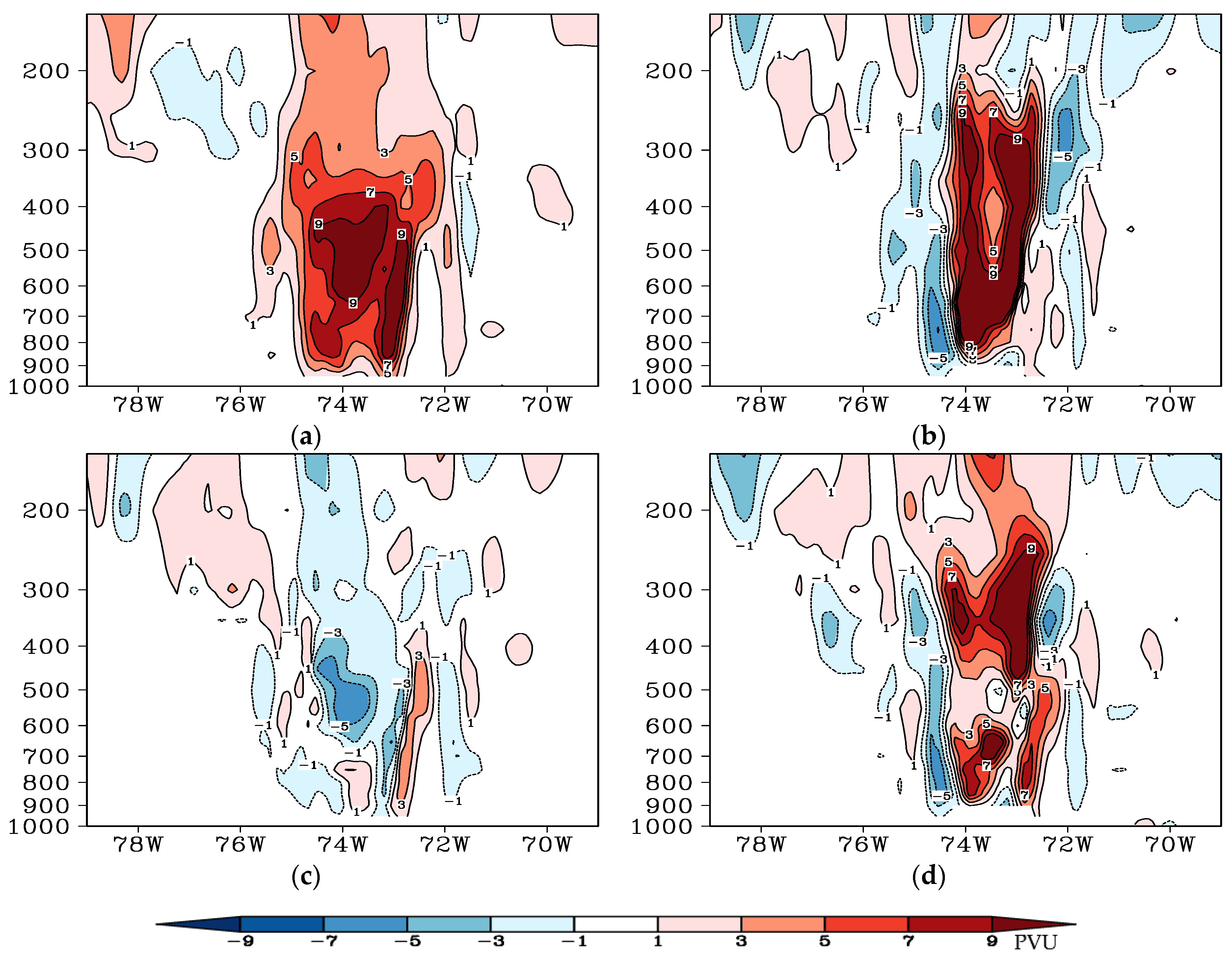
- By assimilating bogus data, the ICs of SLP, pressure perturbation, specific humidity, and PV primarily in the lower atmospheric layers are altered, resulting in a slight intensification of Hurricane Earl’s warm core. Assimilating satellite ozone observations has minimal influence on the ICs, except for the PV pattern in the vicinity of the tropopause. Nonetheless, the assimilation of both satellite ozone and bogus data induces notable alterations in the ICs, extending from the lower to the upper layers. This leads to a more extensive, warmer, and moister core of Hurricane Earl, resulting in a more profound and evenly distributed initial vortex, compared to the scenario where only one type of data is assimilated.
- (2)
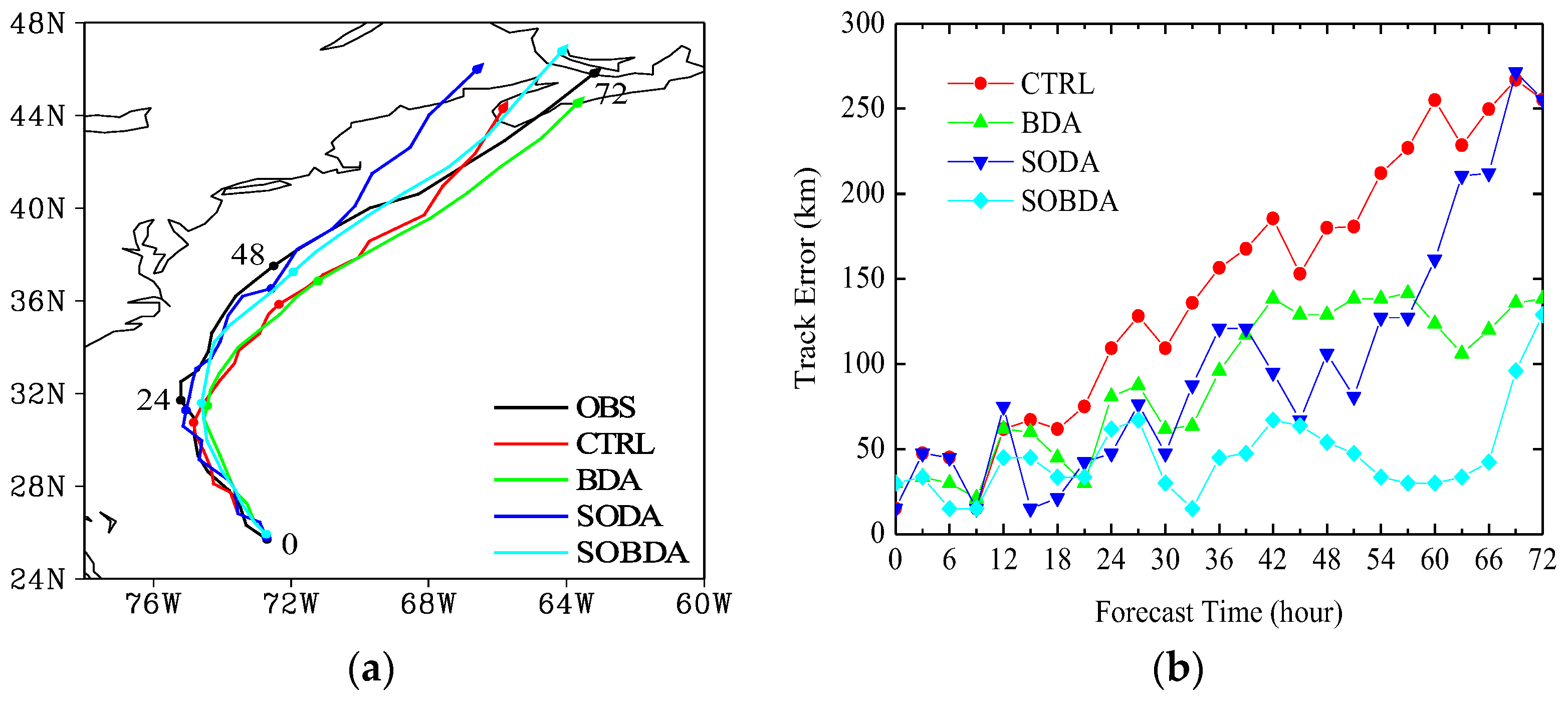
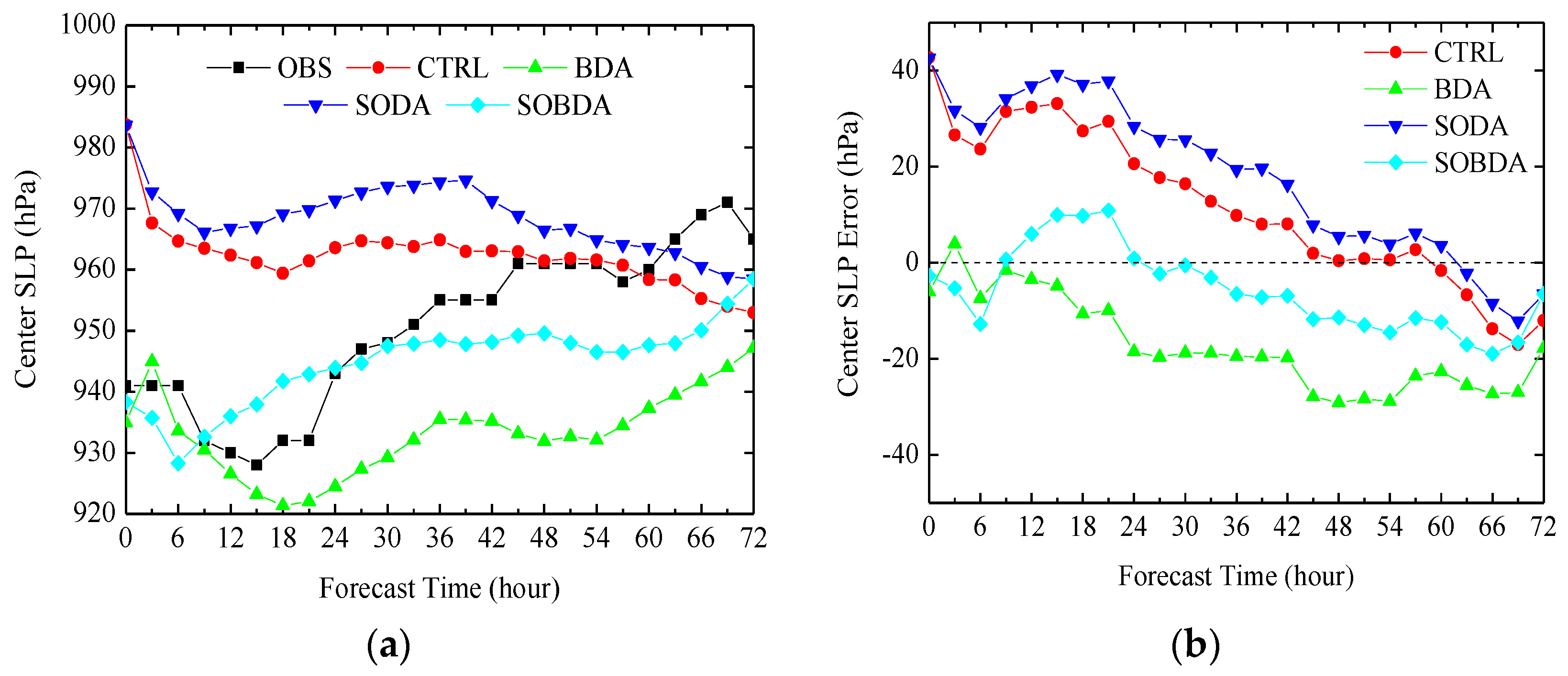
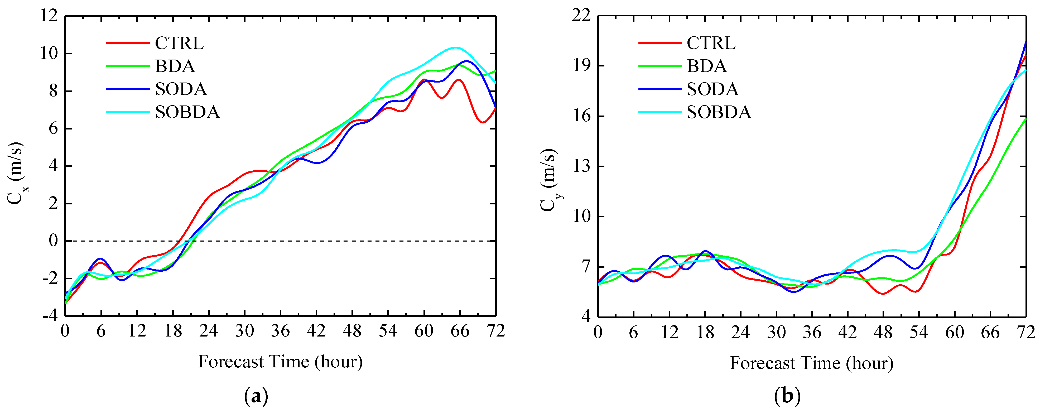
- Changes to the lower levels have a greater effect on hurricane development than modifications to the upper levels. As the integration time passes, the perturbations in the upper levels spread to the lower levels, leading to large discrepancies in the forecasts when satellite ozone and/or bogus data are assimilated. The assimilation of both satellite ozone and bogus data provides a more comprehensive and precise depiction of the hurricane structure features, surpassing the accuracy achieved by assimilating only one type of data or not performing any assimilation. Consequently, the implementation of the SOBDA scheme yields a significant improvement in the accuracy of the hurricane track and intensity forecasts during subsequent numerical simulations.
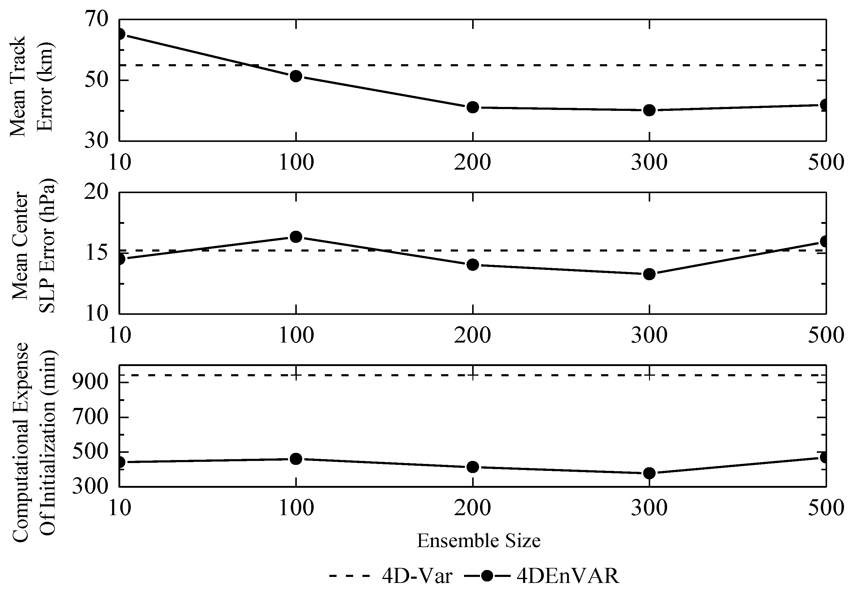
- (3)
- With the 4DEnVar method, hurricane prediction is found to be much more sensitive to the ensemble size. By using the 4DEnVAR method to joint assimilate satellite ozone and bogus data with an appropriate ensemble size, it is possible to significantly enhance hurricane prediction while still consuming a manageable amount of computer resources compared to the 4D-Var method.
Funding
Data Availability Statement
Conflicts of Interest
Appendix A


| Forecast Hours | OBS | CTRL | BDA | SODA | SOBDA | |||||
|---|---|---|---|---|---|---|---|---|---|---|
| LON | LAT | LON | LAT | LON | LAT | LON | LAT | LON | LAT | |
| 0 | 72.70 | 25.70 | 72.71 | 25.79 | 72.72 | 25.92 | 72.71 | 25.79 | 72.72 | 25.92 |
| 3 | 73.30 | 26.30 | 72.91 | 26.44 | 73.06 | 26.43 | 72.91 | 26.44 | 73.06 | 26.43 |
| 6 | 73.50 | 27.20 | 73.54 | 26.80 | 73.27 | 27.22 | 73.54 | 26.80 | 73.42 | 27.21 |
| 9 | 73.80 | 27.80 | 73.76 | 27.72 | 73.61 | 27.73 | 73.63 | 27.86 | 73.63 | 27.86 |
| 12 | 74.40 | 28.60 | 74.25 | 28.09 | 73.84 | 28.52 | 73.81 | 28.25 | 74.00 | 28.64 |
| 15 | 74.70 | 29.30 | 74.32 | 28.75 | 74.06 | 29.31 | 74.66 | 29.13 | 74.22 | 29.30 |
| 18 | 74.80 | 30.10 | 74.55 | 29.55 | 74.30 | 30.11 | 74.59 | 29.95 | 74.44 | 29.96 |
| 21 | 74.80 | 30.90 | 74.78 | 30.21 | 74.53 | 30.90 | 75.13 | 30.58 | 74.52 | 30.77 |
| 24 | 75.20 | 31.70 | 74.83 | 30.74 | 74.43 | 31.46 | 75.05 | 31.27 | 74.60 | 31.58 |
| 27 | 75.20 | 32.50 | 74.59 | 31.44 | 74.34 | 32.14 | 74.95 | 31.83 | 74.51 | 32.27 |
| 30 | 74.70 | 33.00 | 74.33 | 32.01 | 74.09 | 32.85 | 74.86 | 32.52 | 74.42 | 32.96 |
| 33 | 74.40 | 33.80 | 74.06 | 32.57 | 73.81 | 33.41 | 74.76 | 33.07 | 74.33 | 33.65 |
| 36 | 74.30 | 34.60 | 73.64 | 33.29 | 73.54 | 33.98 | 74.32 | 33.52 | 74.22 | 34.21 |
| 39 | 74.00 | 35.30 | 73.52 | 33.84 | 72.93 | 34.70 | 74.06 | 34.22 | 73.79 | 34.93 |
| 42 | 73.60 | 36.20 | 72.92 | 34.57 | 72.32 | 35.42 | 73.83 | 35.34 | 73.18 | 35.65 |
| 45 | 73.10 | 36.80 | 72.65 | 35.41 | 71.86 | 36.14 | 73.40 | 36.19 | 72.56 | 36.38 |
| 48 | 72.50 | 37.50 | 72.35 | 35.84 | 71.21 | 36.85 | 72.57 | 36.52 | 71.93 | 37.24 |
| 51 | 71.80 | 38.20 | 71.54 | 36.56 | 70.55 | 37.43 | 72.12 | 37.51 | 71.29 | 38.10 |
| 54 | 70.80 | 39.10 | 71.06 | 37.13 | 69.70 | 38.14 | 71.82 | 38.21 | 70.62 | 38.81 |
| 57 | 69.70 | 40.00 | 70.04 | 37.86 | 68.84 | 38.85 | 70.81 | 39.08 | 69.76 | 39.67 |
| 60 | 68.30 | 40.60 | 69.72 | 38.56 | 67.95 | 39.55 | 70.14 | 40.08 | 68.69 | 40.66 |
| 63 | 67.10 | 41.70 | 68.13 | 39.69 | 66.86 | 40.66 | 69.64 | 41.48 | 67.41 | 41.78 |
| 66 | 65.80 | 42.90 | 67.59 | 40.94 | 65.91 | 41.77 | 68.54 | 42.61 | 66.26 | 43.17 |
| 69 | 64.50 | 44.30 | 66.65 | 42.34 | 64.73 | 43.00 | 67.99 | 44.01 | 65.23 | 44.97 |
| 72 | 63.20 | 45.80 | 65.84 | 44.28 | 63.68 | 44.51 | 66.60 | 45.97 | 64.13 | 46.76 |


References
- Normand, C. Atmospheric ozone and the upper-air conditions. Q. J. R. Meteorol. Soc. 1953, 79, 39–50. [Google Scholar] [CrossRef]
- Ohring, G.; Muench, H.S. Relationships between ozone and meteorological parameters in the lower stratosphere. J. Atmos. Sci. 1960, 17, 195–206. [Google Scholar] [CrossRef]
- Danielsen, E.F. Stratospheric-tropospheric exchange based on radio-activity, ozone, and potential vorticity. J. Atmos. Sci. 1968, 25, 502–518. [Google Scholar] [CrossRef]
- Shapiro, M.A.; Krueger, A.J.; Kennedy, P.J. Nowcasting the position and intensity of jet streams using a satellite-borne total ozone mapping spectrometer. In Nowcasting; Browning, K., Ed.; Academic Press: Cambridge, MA, USA, 1982; pp. 137–145. [Google Scholar]
- Stout, J.; Rodgers, E.B. Nimbus-7 total ozone observations of western North Pacific tropical cyclones. J. Appl. Meteorol. Climatol. 1992, 31, 758–783. [Google Scholar] [CrossRef]
- Riishøjgaard, L.P.; Källén, E. On the correlation between ozone and potential vorticity for large-scale Rossby waves. J. Geophys. Res. 1997, 102, 8793–8804. [Google Scholar] [CrossRef]
- Davis, C.; Low-Nam, S.; Shapiro, M.A.; Zou, X.; Krueger, A.J. Direct retrieval of wind from Total Ozone Mapping Spectrometer (TOMS) data: Examples from FASTEX. Q. J. R. Meteorol. Soc. 1999, 125, 3375–3391. [Google Scholar] [CrossRef]
- Jiang, X.; Pawson, S.; Camp, C.; Nielsen, J.E.; Shia, R.-L.; Liao, T.; Limpasuvan, V.; Yung, Y.L. Interannual variability and trends of extratropical ozone. Part I: Northern Hemisphere. J. Atmos. Sci. 2008, 65, 3013–3029. [Google Scholar] [CrossRef]
- Carsey, T.P.; Willoughby, H.E. Ozone measurements from eyewall transects of two Atlantic tropical cyclones. Mon. Weather Rev. 2005, 133, 166–174. [Google Scholar] [CrossRef]
- Zou, X.; Wu, Y. On the relationship between Total Ozone Mapping Spectrometer (TOMS) ozone and hurricanes. J. Geophys. Res. 2005, 110, D06109. [Google Scholar] [CrossRef]
- Jang, K.I.; Zou, X.; De Pondeca, M.S.F.V.; Shapiro, M.; Davis, C.; Krueger, A. Incorporating TOMS ozone measurements into the prediction of the Washington, D.C., winter storm during 24–25 January 2000. J. Appl. Meteorol. Climatol. 2003, 42, 797–812. [Google Scholar] [CrossRef]
- Wu, Y.; Zou, X. Numerical test of a simple approach for using TOMS total ozone data in hurricane environment. Q. J. R. Meteorol. Soc. 2008, 134, 1397–1408. [Google Scholar] [CrossRef]
- Liu, Y.; Zou, X. Impact of 4DVAR assimilation of AIRS total column ozone observations on the simulation of Hurricane Earl. J. Meteorol. Res. 2015, 29, 257–271. [Google Scholar] [CrossRef]
- Zou, X.; Xiao, Q. Studies on the initialization and simulation of a mature hurricane using a variational bogus data assimilation scheme. J. Atmos. Sci. 2000, 57, 836–860. [Google Scholar] [CrossRef]
- Xiao, Q.; Zou, X.; Wang, B. Initialization and simulation of a landfalling hurricane using a variational bogus data assimilation scheme. Mon. Weather Rev. 2000, 128, 2252–2269. [Google Scholar] [CrossRef]
- Zhao, Y.; Wang, B.; Wang, Y. Initialization and simulation of a landfalling typhoon using a variational bogus mapped data assimilation (BMDA). Meteorol. Atmos. Phys. 2007, 98, 269–282. [Google Scholar] [CrossRef]
- Xiao, Q.; Chen, L.; Zhang, X. Evaluations of BDA scheme using the Advanced Research WRF (ARW) model. J. Appl. Meteorol. Climatol. 2009, 48, 680–689. [Google Scholar] [CrossRef]
- Park, K.; Zou, X. Toward developing an objective 4DVAR BDA scheme for hurricane initialization based on TPC observed parameters. Mon. Weather Rev. 2004, 132, 2054–2069. [Google Scholar] [CrossRef]
- Zou, X.; Xiao, Q.; Lipton, A.E.; Modica, G.D. A numerical study of the effect of GOES sounder cloud-cleared brightness temperatures on the prediction of Hurricane Felix. J. Appl. Meteorol. Climatol. 2001, 40, 34–55. [Google Scholar] [CrossRef]
- Pu, Z.; Tao, W.-K.; Braun, S.; Simpson, J.; Jia, Y.; Halverson, J.; Olson, W.; Hou, A. The impact of TRMM data on mesoscale numerical simulation of Supertyphoon Paka. Mon. Weather Rev. 2002, 130, 2448–2458. [Google Scholar] [CrossRef]
- Amerault, C.; Zou, X. Preliminary steps in assimilating SSM/I brightness temperatures in a hurricane prediction scheme. J. Atmos. Ocean. Technol. 2003, 20, 1154–1169. [Google Scholar] [CrossRef]
- Zhao, Y.; Wang, B.; Ji, Z.; Liang, X.; Deng, G.; Zhang, X. Improved track forecasting of a typhoon reaching landfall from four-dimensional variational data assimilation of AMSU-A retrieved data. J. Geophys. Res. 2005, 110, D14101. [Google Scholar] [CrossRef]
- Zhang, X.; Xiao, Q.; Fitzpatrick, P.J. The impact of multisatellite data on the initialization and simulation of Hurricane Lili’s (2002) rapid weakening phase. Mon. Weather Rev. 2007, 135, 526–548. [Google Scholar] [CrossRef]
- Wang, Y.; Wang, B.; Fei, J.; Han, Y.; Ma, G. The effects of assimilating satellite brightness temperature and bogus data on the simulation of Typhoon Kalmaegi (2008). J. Meteorol. Res. 2013, 27, 415–434. [Google Scholar] [CrossRef]
- Liu, Y.; Zhang, W. Improved hurricane forecasting from a variational bogus and ozone data assimilation (BODA) scheme: Case study. Meteorol. Atmos. Phys. 2016, 128, 715–732. [Google Scholar] [CrossRef]
- Gong, Y.; Liang, K.; Wu, X.; Shao, Q.; Li, W.; Liu, S.; Han, G.; Liu, H. An application of the A-4DEnVar to coupled parameter optimization. Acta Oceanol. Sin. 2022, 41, 60–70. [Google Scholar] [CrossRef]
- Liang, K.; Li, W.; Han, G.; Shao, Q.; Zhang, X.; Zhang, L.; Jia, B.; Bai, Y.; Liu, S.; Gong, Y. An analytical four-dimensional ensemble-variational data assimilation scheme. J. Adv. Model. Earth Syst. 2021, 13, e2020MS002314. [Google Scholar] [CrossRef]
- Fairbairn, D.; Pring, S.R.; Lorenc, A.C.; Roulstone, I. A comparison of 4DVar with ensemble data assimilation methods. Q. J. R. Meteorol. Soc. 2014, 140, 281–294. [Google Scholar] [CrossRef]
- Arbogast, É.; Desroziers, G.; Berre, L. A parallel implementation of a 4DEnVar ensemble. Q. J. R. Meteorol. Soc. 2017, 143, 2073–2083. [Google Scholar] [CrossRef]
- Yang, Y.; Mémin, E. High-resolution data assimilation through stochastic subgrid tensor and parameter estimation from 4DEnVar. Tellus A 2017, 69, 1308772. [Google Scholar] [CrossRef]
- Song, H.J.; Kang, J.H. Effects of the wind-mass balance constraint on ensemble forecasts in the hybrid-4DEnVar. Q. J. R. Meteorol. Soc. 2019, 145, 434–449. [Google Scholar] [CrossRef]
- Han, G.; Wu, X.; Zhang, S.; Liu, Z.; Navon, I.M.; Li, W. A study of coupling parameter estimation implemented by 4D-Var and EnKF with a simple coupled system. Adv. Meteorol. 2015, 2015, 530764. [Google Scholar] [CrossRef]
- Tian, X.; Feng, X. A non-linear least squares enhanced POD-4DVar algorithm for data assimilation. Tellus A 2015, 67, 25340. [Google Scholar] [CrossRef]
- Tian, X.; Zhang, H.; Feng, X.; Xie, Y. Nonlinear least squares En4DVar to 4DEnVar methods for data assimilation: Formulation, analysis, and preliminary evaluation. Mon. Weather Rev. 2018, 146, 77–93. [Google Scholar] [CrossRef]
- Bian, J.; Gettelman, A.; Chen, H.; Pan, L.L. Validation of satellite ozone profile retrievals using Beijing ozonesonde data. J. Geophys. Res. 2007, 112, D06305. [Google Scholar] [CrossRef]
- Monahan, K.P.; Pan, L.L.; McDonald, A.J.; Bodeker, G.E.; Wei, J.; George, S.E.; Barnet, C.D.; Maddy, E. Validation of AIRS v4 ozone profiles in the UTLS using ozonesondes from Lauder, NZ and Boulder, USA. J. Geophys. Res. 2007, 112, D17304. [Google Scholar] [CrossRef]
- Pan, L.L.; Bowman, K.P.; Shapiro, M.; Randel, W.J.; Gao, R.S.; Campos, T.; Davis, C.; Schauffler, S.; Ridley, B.A.; Wei, J.C.; et al. Chemical behavior of the tropopause observed during the Stratosphere-Troposphere Analyses of Regional Transport experiment. J. Geophys. Res. 2007, 112, D18110. [Google Scholar] [CrossRef]
- Pittman, J.V.; Pan, L.L.; Wei, J.C.; Irion, F.W.; Liu, X.; Maddy, E.S.; Barnet, C.D.; Chance, K.; Gao, R.-S. Evaluation of AIRS, IASI, and OMI ozone profile retrievals in the extratropical tropopause region using in situ aircraft measurements. J. Geophys. Res. 2009, 114, D24109. [Google Scholar] [CrossRef]
- Zhao, H.; Shu, Y.; Mao, Y.; Liu, Y.; Yu, K. The Assimilation Effect of Multi-New Types Observation Data in the Forecasts of Meiyu-Front Rainstorm. Atmosphere 2023, 14, 693. [Google Scholar] [CrossRef]
- Shu, A.; Shen, F.; Jiang, L.; Zhang, T.; Xu, D. Assimilation of Clear-sky FY-4A AGRI radiances within the WRFDA system for the prediction of a landfalling Typhoon Hagupit (2020). Atmos. Res. 2023, 283, 106556. [Google Scholar] [CrossRef]
- Rodgers, E.B.; Stout, J.; Steranka, J.; Chang, S. Tropical cyclone-upper atmospheric interaction as inferred from satellite total ozone observations. J. Appl. Meteorol. Climatol. 1990, 29, 934–954. [Google Scholar] [CrossRef]
- Bosart, L.F. Tropopause folding: Upper-level frontogenesis and beyond. In A Half Century of Progress in Meteorology: A Tribute to Richard Reed; Springer: Berlin/Heidelberg, Germany, 2003; pp. 13–47. [Google Scholar]
- Song, L.; Shen, F.; Shao, C.; Shu, A.; Zhu, L. Impacts of 3DEnVar-Based FY-3D MWHS-2 Radiance Assimilation on Numerical Simulations of Landfalling Typhoon Ampil (2018). Remote Sens. 2022, 14, 6037. [Google Scholar] [CrossRef]
- Qing, Z.; Zeng, Q.; Wang, H.; Liu, Y.; Xiong, T.; Zhang, S. ADASYN-LOF Algorithm for Imbalanced Tornado Samples. Atmosphere 2022, 13, 544. [Google Scholar] [CrossRef]
- Liu, Y.; Zou, X. Quality control of AIRS total column ozone data within tropical cyclones. Front. Earth Sci. 2016, 10, 222–235. [Google Scholar] [CrossRef]
- Fujita, T. Pressure distribution within a typhoon. Geophys. Mag. 1952, 23, 437–451. [Google Scholar]
- Grell, G.A.; Dudhia, J.; Stauffer, D.R. A Description of the Fifth Generation Penn State/NCAR Mesoscale Model (MM5). In NCAR Technical Note; NCAR: Boulder, CO, USA, 1994; p. 117. [Google Scholar]
- Dong, K.; Neumann, C.J. On the relative motion of binary tropical cyclones. Mon. Weather Rev. 1983, 111, 945–953. [Google Scholar] [CrossRef]
- Velden, C.S.; Leslie, L.M. The basic relationship between tropical cyclone intensity and the depth of the environmental steering layer in the Australian region. Weather Forecast. 1991, 6, 244–253. [Google Scholar] [CrossRef]
- Holland, G.J. Tropical cyclone motion: A comparison of theory and observation. J. Atmos. Sci. 1984, 41, 68–75. [Google Scholar] [CrossRef]
- Wang, B.; Elsberry, R.L.; Wang, Y.; Wu, L. Dynamics in tropical cyclone motion: A review. Chin. J. Atmos. Sci. 1998, 22, 535–547. (In Chinese) [Google Scholar]


| Mean Error (DU) | Standard Deviation (DU) | Correlation Coefficient (AIRS Ozone and MPV) | |
|---|---|---|---|
| Prior to quality control | −2.3243 | 23.3862 | 0.5428 |
| Following quality control | 1.2473 | 14.2231 | 0.8801 |
| Model Layer | ||
|---|---|---|
| 193 hPa ( = 0.15) | −1.98 | 275.54 |
| 231 hPa ( = 0.19) | −3.62 | 276.21 |
| 269 hPa ( = 0.23) | −3.38 | 276.31 |
| 307 hPa ( = 0.27) | −3.21 | 276.47 |
| 345 hPa ( = 0.31) | −3.33 | 276.70 |
Disclaimer/Publisher’s Note: The statements, opinions and data contained in all publications are solely those of the individual author(s) and contributor(s) and not of MDPI and/or the editor(s). MDPI and/or the editor(s) disclaim responsibility for any injury to people or property resulting from any ideas, methods, instructions or products referred to in the content. |
© 2023 by the author. Licensee MDPI, Basel, Switzerland. This article is an open access article distributed under the terms and conditions of the Creative Commons Attribution (CC BY) license (https://creativecommons.org/licenses/by/4.0/).
Share and Cite
Liu, Y. A Hurricane Initialization Scheme with 4DEnVAR Satellite Ozone and Bogus Data Assimilation (SOBDA) and Its Application: Case Study. Atmosphere 2023, 14, 866. https://doi.org/10.3390/atmos14050866
Liu Y. A Hurricane Initialization Scheme with 4DEnVAR Satellite Ozone and Bogus Data Assimilation (SOBDA) and Its Application: Case Study. Atmosphere. 2023; 14(5):866. https://doi.org/10.3390/atmos14050866
Chicago/Turabian StyleLiu, Yin. 2023. "A Hurricane Initialization Scheme with 4DEnVAR Satellite Ozone and Bogus Data Assimilation (SOBDA) and Its Application: Case Study" Atmosphere 14, no. 5: 866. https://doi.org/10.3390/atmos14050866