1. Introduction
The butterfly effect described by Edward Lorenz [
1,
2] has become a central concept in the study of nonlinear systems. This effect is typically associated with “chaos” and characterized by positive Lyapunov exponents. Of course, the Lyapunov exponents of a trajectory are a partial description of what happens near the trajectory based on a linearization of the dynamics near the trajectory. That analysis is greatly simplified if the system is linear since the linearization of all trajectories is the same. By studying linear systems, we gain clarity about the relationship between Lyapunov exponents and the butterfly effect, which can be quantified by what we call the “butterfly number” in
Section 2. By presenting a butterfly effect in simple linear systems, we hope to contribute to a deeper understanding of the role of dimensionality and off-diagonal terms in the linearization of the dynamics of physical systems. We are not creating a new butterfly effect here, but we are simply pointing out how it can occur in systems for which there is no positive exponent, and we use only elementary mathematical techniques.
Sensitive dependence on initial conditions. There are several ways of characterizing sensitive dependence on initial conditions [
3,
4,
5]. Sensitive dependence on initial conditions is defined by J. Guckenheimer [
5] in any dimension as follows: there exists a positive
such that, for all
x in the phase space and all
, there is some
y that is within a distance
of
x and there is some
n such that
The phrase “sensitive dependence on initial conditions” was used by D. Ruelle [
6] to indicate some exponential rate of divergence of the orbits of nearby points, which has often been used to characterize chaos in the literature. Guckenheimer’s definition does not require there to be a positive Lyapunov exponent, but it is challenging to find a natural system that satisfies their definition but has no trajectories with a positive Lyapunov exponent.
The ancient history of sensitivity to initial conditions. The following seems to describe how a tiny perturbation can lead to large changes through a pattern of increasingly big effects over a finite amount of time. Benjamin Franklin included a version of the tale about horseshoes and battles in their Poor Richard’s Almanack. Franklin’s was far from the first version. (Benjamin Franklin, Poor Richards Almanack, June 1758, The Complete Poor Richard Almanacks, facsimile ed., vol. 2, pp. 375–377) [
7].
The horseshoe nail cascade effect: “For Want of a Nail”, an example of “finite-time sensitive dependence”
For want of a nail the shoe was lost;
For want of a shoe the horse was lost;
For want of a horse the rider was lost;
For want of a rider the message was lost;
For want of a message the battle was lost;
For want of a battle the kingdom was lost;
Furthermore, all for the want of a horseshoe nail.
We believe that scientists and mathematicians were among the last people to learn about sensitivity to initial conditions. The above nail tale has been discussed by other authors, including Lorenz [
8] and Shen [
9]. We mention it here to contrast it with our “parable about angles” in
Section 3.
Dynamics of the Lorenz’s 1969 paper [2]. The Lorenz paper from 1969 analyzed a high dimensional spatial multi-scale model, describing how energy at the model’s smallest scales could propagate quickly to the largest scales, provided there was lots of energy in the smallest scales. Perhaps huge numbers of energetic butterflies could provide that energy, although the article did not mention butterflies. Wikipedia’s “butterfly effect” [
10] says: “According to Lorenz, when he failed to provide a title for a talk he was to present at the 139
th meeting of the American Association for the Advancement of Science in 1972, Philip Merilees concocted ‘Does the flap of a butterfly’s wings in Brazil set off a tornado in Texas?’ as a title.” A single flapping of a butterfly causes chaos in the Lorenz paper from 1963 [
1], whereas the butterfly effect in the Lorenz paper from 1969 [
2] is caused by the propagation of huge numbers of flapping butterflies. The analysis of the Lorenz’s 1969 model’s linearly unstable solutions was first documented in Shen et al. [
11].
Outline of the paper. In
Section 2, we begin with a mosquito model instead of a butterfly. We introduce a simple linear one-space-dimension map. We show that the map shows a butterfly effect, “the sensitive dependence on initial conditions” for some finite times, although the map is not chaotic in the sense that it does not have positive Lyapunov exponents. In
Section 3, we describe another well-known multi-dimensional torus map where the coordinates are angles. We investigate the numerics of the map in
Section 4. In
Section 5, we explain the known mathematical results and introduce a conjecture together with some numerical evidence. We discuss the related works and summarize our results in
Section 6.
2. Linear -Dimensional System Showing the Butterfly Effect
Models for the spread of Zika-infected mosquitoes. Jeffery Demers et al. [
12] investigated a heterogeneous, two-space-dimensional model of infected Aedes mosquitoes. Some species of mosquitoes, such as Aedes, can become infected and can transmit diseases such as Zika, and they have little mobility during their lifetimes. This means it can be effective to focus the killing of mosquitoes in the small areas where the disease exists. See our discussion section (
Section 6.2) for New York Times articles that discuss the Zika outbreak in Miami, Florida, and elsewhere. The World Health Organization recently declared mosquito-borne Zika an “international public health emergency”. Our focus is on how a new exponentially growing outbreak is local early in the outbreak. Hence, a new outbreak can sometimes be interrupted using only local strategies for killing mosquitoes, as opposed to expensive strategies that would try to (temporarily) eradicate mosquitoes in a large region. Of course, “exponential growth” is temporary. Our model is spatially one-dimensional, but it is easy to convert it into a two-space dimension model, provided the winds generally blow mosquitoes in one direction.
A one-space-dimensional infected-mosquito model. We assume that there is a line of land tracts numbered
, perhaps along a road. We imagine that these regions all have a similar area, perhaps one square hectare. Our model’s infected mosquitoes live for one time period, and in one time period, each infected mosquito in tract
k has
progeny, which we imagine is approximately 2. We assume
mosquitoes stay in tract
k and
are blown by a constant wind into tract
. Writing
for the number of infected mosquitoes in tract
k yields the following dynamical model, which we call our “(infected-) mosquito model”.
This equation can be viewed as a linearization about
for all coordinates
j—of a spatial logistic-based map. One possibility uses
where
is a density at each tract
k with a maximum sustainable value of 1. The nonlinear equation is the following:
Recall that is a density while is the number of mosquitoes. Huge values of correspond to moderate values of .
We can write (
1) in vector format, writing
. For time
, let
be a trajectory of (
1) determined by
where we define
as follows:
There can be rapid growth over time for large K when for all k. We invite the reader to try various choices of coefficients. This model gives many cases to consider.
Notation for “spatially homogeneous” matrices. Tri-diagonal matrix. In this part, we comment on the case where a map is determined by the tri-diagonal matrix
. Assume that the
matrix
is a tri-diagonal matrix with the following form:
where
a,
b, and
c are non-negative real numbers. This type of matrix is considered to commonly appear in a linearized system in various nonlinear phenomena. An example with a linearization that is somewhat similar is the Gledzer–Okhitani–Yamada (GOY) shell model of fluid turbulence that mimics the Galerkin spectral equations of the Navier–Stokes equations (A detailed analysis of this matter will be reported elsewhere as a joint work with Miki U. Kobayashi.). It is a system of
N-dimensional complex-valued ordinary differential equations with the following form [
13]:
where
f is a forcing parameter,
is a Kronecker delta, and
, and
with
for other
n.
The eigenvalues the matrix
are
the
Lyapunov number is
, and the Lyapunov exponent is the log of the Lyapunov number. From this formula, we obtain an inequality:
See [
14] for details. For large
K,
. Of course if
, the right-hand side is
.
Define the
butterfly number (or
the local Lyapunov number) of the tri-diagonal matrix to be the column sum of the typical column of the matrix,
For positive
,
which is the largest Lyapunov number. Hence, the temporary growth rate is
. If
and
, the infected mosquitoes double each generation (until the open boundary at tract
K is reached) while the Lyapunov number is 0 (and the Lyapunov exponent is
. If
has no negative entries and the first and last entries are 0, then
where
. Hence, the sum of the entries increases by a factor of
from one application of
.
To focus on a truly elementary case, we focus on the case where all and or, even more simply , and .
Our model still has a one-space dimension and is spatially homogeneous (except at entries 1 and
K).
the one-mosquito-generation map with
K land tracts. Assume that, at time 0, there is one infected mosquito, and it is in tract 1.
As we describe later, tract
k at time
n for
will have
infected mosquitoes. Recall that
, which is 0 if
.
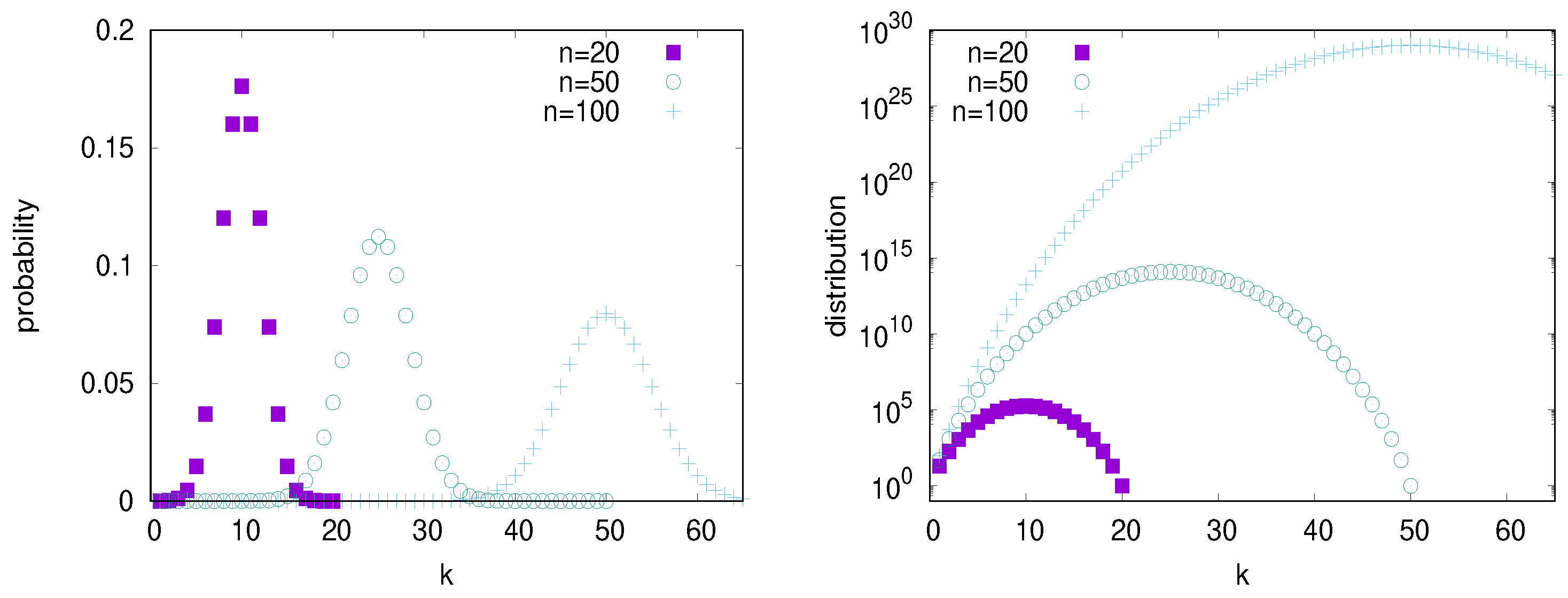
Figure 1 displays the distribution. It seems to show a pattern analogous to the pipe flow [
15], where the center of the distribution at time
n is tract
. Of course, pipe flow is a nonlinear process, while our model emphasizes only the linear growth phase. See our remarks in
Section 6 on the work of Kaneko and Crutchfield on pipe flow. Later, we discuss how the center of the infected mosquito distribution moves, as seen in
Figure 1. Clearly, in reality, the population of infected mosquitoes exists against a background of a large uninfected population. The number of infected mosquitoes would eventually saturate, a fact not reflected in our model.
One infected Miami mosquito. We examine a finite line of K tracts where all , so eventually, if n is large, the largest value of occurs at the end, i.e., at . In Miami, the winds tend to blow from west to east, and since Miami is on the western edge of the Atlantic Ocean, its mosquitoes in the last tract can be blown into the ocean and cease to be a problem. We assume an outbreak starts with one mosquito infected with the Zika virus. Here, we aim at simplicity. A more detailed model such as Demers’ would be spatially heterogeneous and two-dimensional, which would include people infecting mosquitoes and mosquitoes infecting people. The resulting behavior could be similar to the explosive growth we observe here, depending on the details, possibly growing even faster.
Again, we can write (
9) in vector format, writing
. For time
, let
be a trajectory of (
9) determined by
where
M is the two-diagonal matrix
matrix
, i.e.,
.
Let denote the vector whose entry is 1 and its other entries are 0. The finite-dimensional matrix M (with dimension K) has only one eigenvector, , and its eigenvalue is 1, so all of the map’s Lyapunov exponents are 0. The multiplicity of the eigenvector is K. The matrix M is a Jordan block matrix.
The time mosquito distribution for Equation (10). The natural initial condition for the mosquito model is
. For this initial state
, i.e., one mosquito in tract 1 at time 0, the number of infected mosquitoes at any later time
on tract
k where
is
, and the total number of infected mosquitoes is
provided
.
The vector at time n is the left-most column of , and its last coordinate is , which, of course, is 0 for . Since K is fixed, grows slower than exponentially as n increases.
If the last coordinate
is 0 at time
n, then the total number of infected mosquitoes at time
is twice the total at time
n, i.e., for time
n,
In this case, generally, when time
n is less than
K, the mosquitoes have not yet reached the last tract,
K, and the application of
M doubles the sum. See
Figure 1 (right). As mentioned above, there is only one eigenvector of
M, and that is
i.e., all entries except the last are 0, and the last is one. This is an eigenvector with an eigenvalue of 1 with a multiplicity of
K. Hence, the rapid growth of the sum of the coordinates seen in Equation (
11) is not because of the eigenvalue but is
a result of the off-diagonal terms that do not contribute to the eigenvalues. While Lyapunov exponents come from linearizations, they do not reflect all of the information in the linearization. Since our map is linear, this point is easier to see.
3. Converting Each into a Direction on a Circle
Skew-product map of a torus. The special mosquito map can be converted into a well-known “skew-product map” on a torus. Each becomes an angle in a circle that we represent by , and we identify the ends, 0 and 1, by computing each . In a physics context, angles are often referred to as phases.
It is traditional to include an irrational
, in the rotation map on the first circle
,
and having
irrational is required for the results in
Section 5. We also obtain maps of any finite dimension, including the long-studied two-dimensional map on the two-torus
[
16,
17,
18,
19],
where, in this paper, “
” signifies that
is always applied to each coordinate of a vector
v.
We investigate the map of the
K-dimensional torus
because it exhibits a butterfly effect (via the perturbation of angles):
where
K is fairly large, perhaps
. We choose 24 for illustrations because the width of Texas is approximately
times the size of a 3 cm. butterfly.
Each coordinate value,
, is a point on a circle, so we can refer to it as a “direction” or an angle. Each perturbation of direction
on iterate
n perturbs the direction
on iterate
and later. We make a conjecture about the behavior of this equation in
Section 5. Write
, and for
, let
be a trajectory of (
14).
Notice that the
coordinate at time
n, namely
, only depends on
for
, so that
is a trajectory of (
14), and for
, it is a vector of length 2, so then it is a trajectory of (
13). Writing (
14) in vector format
Notice that because all entries of M are integers, the map (applying only after n applications of M) is identical to , applying at each iterate. Furthermore, if we make numerical studies in which each coordinate remains less than 1, the results are meaningful regardless of whether is applied.
A parable about angles. This part is about angles or orientations. We now propose a parable about changing directions, where one orientation of something causes a change in the orientation of something larger. Imagine a lot of activity in a flat field with a butterfly, a bird, a cat, a dog, a person, a bike, a car, and a truck, all traveling in different directions. The direction of each is a point in a circle, collectively a point on an eight-dimensional torus .
A butterfly flaps its wings;
a nearby bird changes direction;
a running cat watching the bird swerves;
a dog swerves at the motion of the cat;
a walking person swerves to avoid hitting the dog;
a passing bicycle swerves a bit;
causing a passing car to change its direction;
a truck changes directions in response.
The butterfly flapping its wings cascades to ever larger scales, perhaps to Texas-sized scales containing tornadoes. All of these changes in directions need not affect the energy of each component. Or we can follow Lorenz, who investigates packets of air of different sizes, small packets perturbing larger packets, in increasing sequence of increasingly large air packets. Each packet is twice the diameter of its predecessor [
2]. Tiny initial perturbations throughout the small-scale packets grow quickly and together become a large-scale perturbation. In this sense, one butterfly flapping its wings in the smallest packet under consideration totally changes the direction of the largest-scale tornado environment, shifting the tornado perhaps from Oklahoma to Texas, or vice versa. Oklahoma and Texas are adjacent states in the USA. These are among the places in the world with the most severe tornado weather.
The perturbations keep influencing the larger scales, adding ever-increasing perturbations to the direction of the next larger packet. The time scale for the perturbations to occur is shorter for the small scales than for the larger scales, but we ignore this inconsistency.
4. Numerical Investigations
We use a superscript to denote the iterate number of vectors such as
and
and a subscript for coordinate number. Choose initial vectors
so that only the first coordinates (denoted by subscripts) have a difference:
, and for coordinate
,
. We find that the 20
th coordinate of the 300
th iterate of
M is approximately
, i.e.,
Note that the value is the maximum possible difference since and are in a circle where the maximum distance between two points is .
We can think of different
s as representing behaviors at different scales of different swirls in the atmosphere, consecutive scales representing the size differences of a factor of 2. Perhaps we can say that a typical butterfly has a size of roughly
meters, while tornado weather patterns have a scale of at least
meters, which is the approximate width of Texas. These differ by roughly
(or more precisely
). Each swirl can change the direction of the next higher swirl. In order to realistically scale the butterfly problem is
for our skew-product system Equation (
14). Each swirl might be twice the scale of the next smaller scale.
Of course, there is an immense number of air packets that are the size of a butterfly, and perturbations in each might affect some next larger packet. An intermediate-size packet might be perturbed by several smaller packets. However, here, we look only at a single cascade starting with one butterfly, and for each packet, we only look at its influence on one larger packet. Realistically, the time of propagation from the packet to the larger is longer as k increases, a fact that our maps do not reflect.
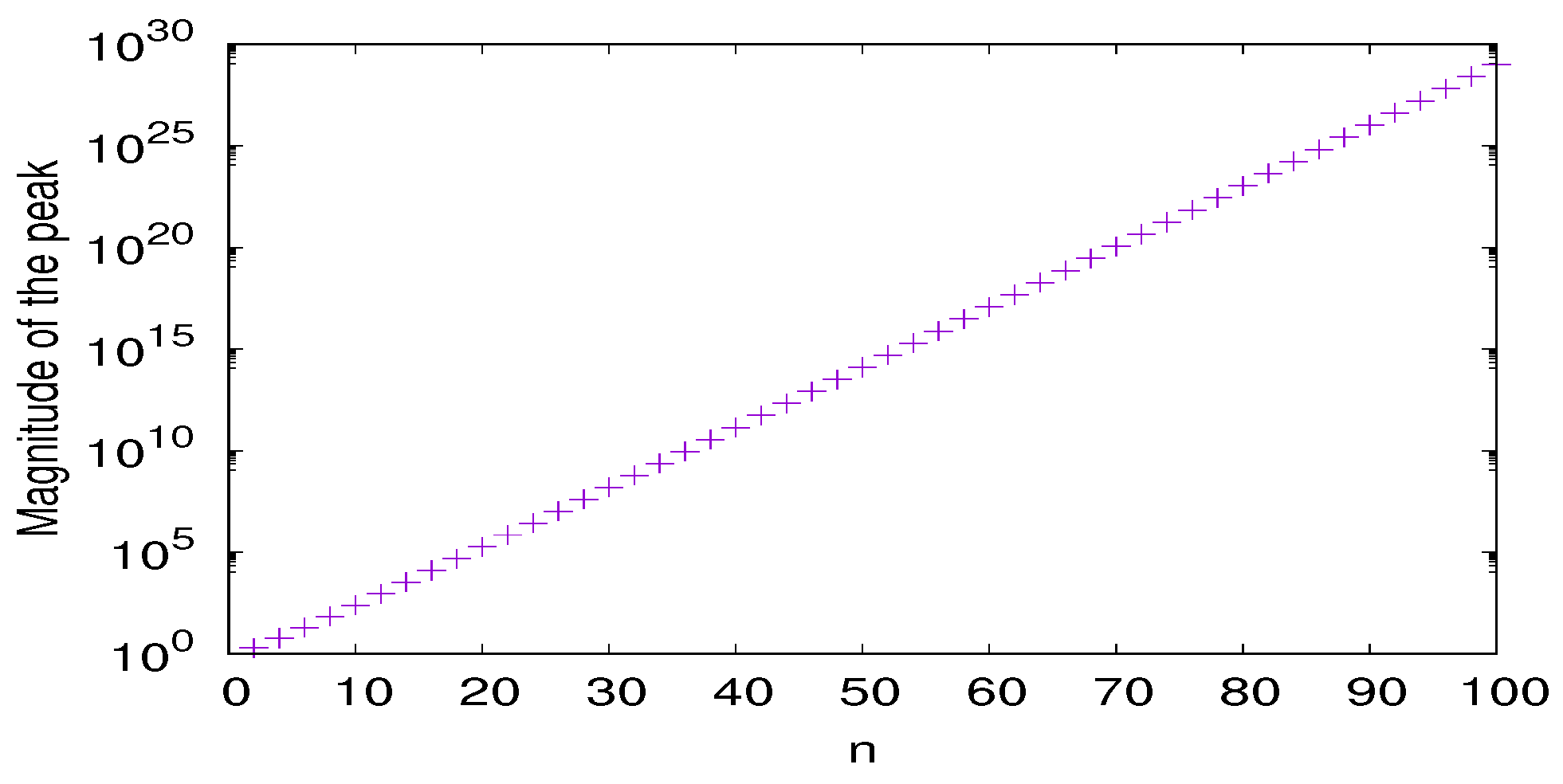
A moving peak of the distribution. In the following
Table 1, define
for
. It is the magnitude of the largest coordinate of
where
for the case of unbounded space. Hence the location of the peak value is at
. This location moves to larger values as time
n increases.
The number
is a finite-time geometric growth rate (which approaches 2 as can be seen in the table). This value approaches 2, but it is showing that as
n increases, some circle (namely circle #
) is strongly affected by the initial tiny perturbation. See also
Figure 2.
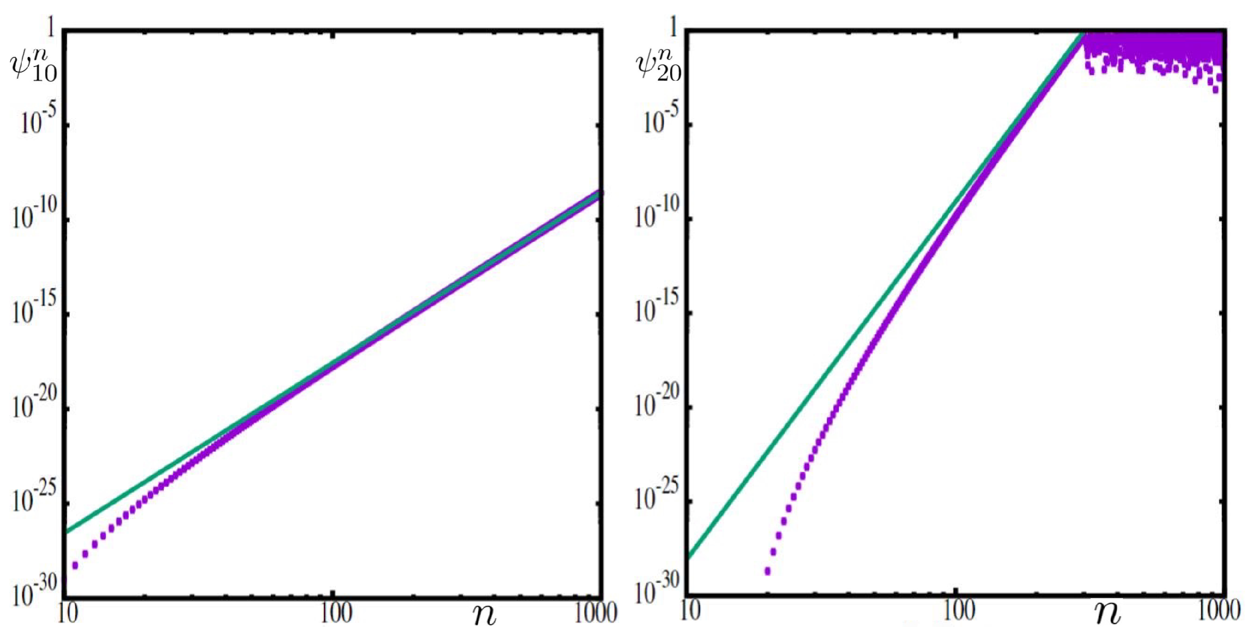
Sensitivity is about the behavior of the difference between two different trajectories. Since the equations we study are linear, we can write the equations for such a difference. Let
where
and
are two trajectories. Then, the difference
satisfies
This equation without
is the mosquito model (
9). In that case, the sum of coordinates of
doubles each iterate in the unbounded case where
K is infinite. We consider two trajectories whose initial conditions differ only in the first coordinate. In
Figure 3, we see the growth in the difference in coordinate
k of
between two trajectories with respect to
n. It asymptotically converges to an exponential growth.
5. Occasional Closest Approach of Two Trajectories
In this section, we discuss the mathematical aspects of the map
F in Equation (
14) concerning the degree of complexity.
Scrambled pairs. For a map
F, we say a pair
of points in the space is
scrambled [
20] if
For the map Equation (
14), the first coordinate of
is independent of
n. Hence, the infimum of the distance between
and
could go to zero only if we choose two points with the same first coordinate.
Let
be a set of pairs of points. Let
denote the maximum possible distance between pairs in
. We say a pair
in
is
totally scrambled (in
) if the pair is scrambled and satisfies
Conjecture 1. For the map Equation (
14)
on for
, let be the set of pairs whose first coordinates are equal. Then, almost every pair in is totally scrambled. We describe the numerical evidence for this conjecture later in this section. Notice that is invariant: for each pair in , the pair is in for all .
Results for the map Equation (14) when is irrational. The following theorems by Furstenberg [
19] are fundamental results for the map (
14). See also Furstenberg Theorem 4.21 (p. 116) and Corollary 4.22 of the book [
18].
Theorem 1. The map is minimal (every orbit is dense).
Recall: A Borel set is any set that can be formed from open sets through the operations of countable union, countable intersection, and complements.
Theorem 2. The map is uniquely ergodic (there is only one invariant Borel probability measure).
Since the map Equation (
14) preserves the Lebesgue measure, its unique ergodicity implies its minimality. In general, minimality does not imply unique ergodicity, for example, interval exchange transformations (IET).
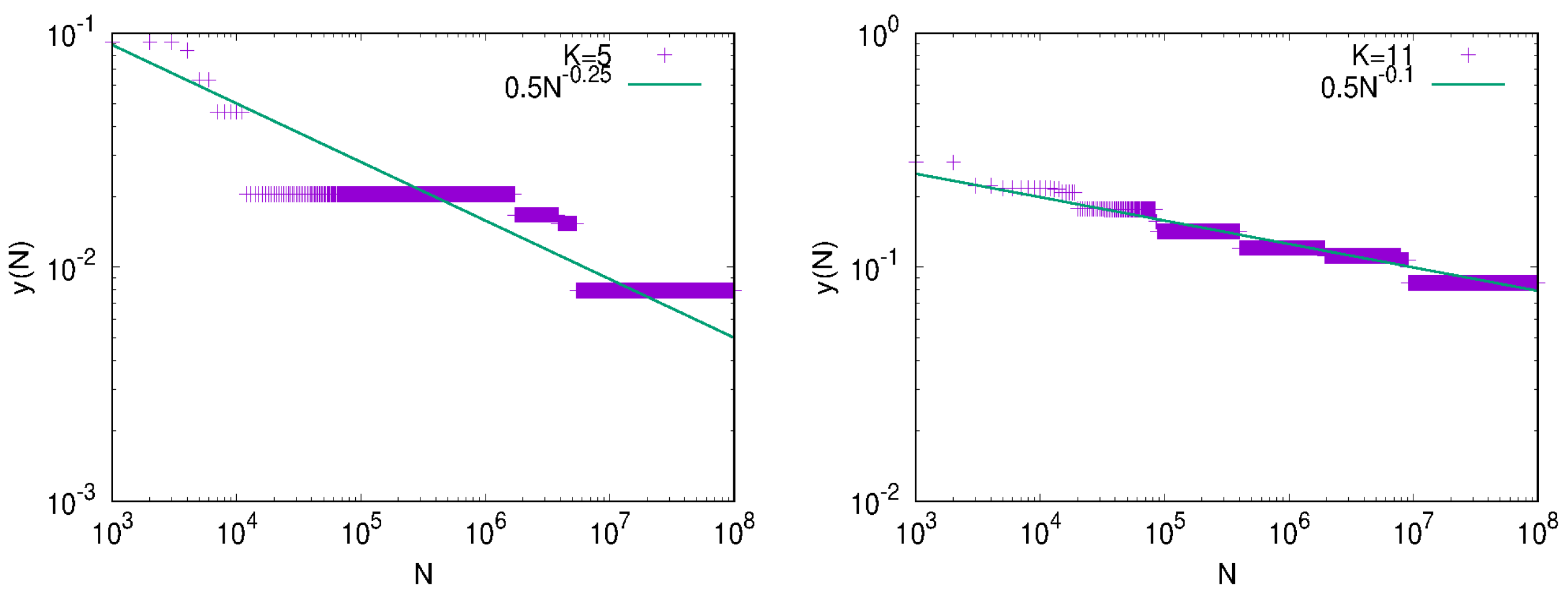
Numerical evidence for our conjecture. Two trajectories might occasionally move close together, only to diverge, repeating this pattern in a non-periodic or apparently stochastic manner. In
Figure 4, we can see that the closest approach
between two trajectories during the time interval
decreases as time
N increases and converges to 0. It supports the first condition of the above conjecture. The decay rate of the closest difference at time
N seems to obey a power law which can be explained below. Suppose we choose
N random points using a uniform distribution on a
D-dimensional box
. For
, when choosing
N random independent points, the expected number of points in
is
. If we choose
so that the expected number is 1, we obtain
, i.e.,
. In our case,
. Thus, we plot
on a log-log scale which yields a straight line
with slope
For such an
, given
N, the probability that none of the
N points are in the
is
.
Figure 4 shows that the difference between two trajectories behaves in this manner. Note that, if two values of
N are chosen close together, whether the plotted points on curves are above or below the line is correlated.


