1. Introduction
The current field of atmospheric sciences has its main roots in traditional meteorology, and the mainstream studies during the “formation period” of modern meteorology in the early 20th century (for example, Bjerknes, 1919) [
1] were undoubtedly synoptic meteorology, which concerns the large-scale motion of the lower atmosphere. During those days, small-scale motions such as convections were mostly ignored in the analysis as they did not seem to be relevant to the motions of air masses, which are usually larger than a few thousand km in horizontal dimension. It was later (e.g., Riehl and Markus, 1958 [
2]; see also Yanai and Johnson, 1993 [
3], for a later review) that convective scale motions received more attention and the importance of vertical motions to the formation of clouds and their impact on the thermodynamics of the atmosphere were more widely studied. Earlier studies of convective scale motions tended to focus more on the dynamics side, although it was well-known that various microphysical processes, especially those involving the phase change of water substances that either release or consume latent heat, can have a significant impact on the cloud behavior (Byers, 1965 [
4]). Convection scale motions are usually considered “mesoscale” phenomena with dimensions of usually tens to hundreds of km as opposed to 1000 km or more for the synoptic scale. Cloud microphysics operates at a scale even smaller than the convection scale, and the most fundamental cloud microphysical processes such as nucleation and crystallization operate at submicron or smaller scales (Fletcher, 1962 [
5]; Pruppacher and Klett, 2010 [
6]; Wang, 2013 [
7]). These processes are justifiably called microscale.
Because of the wide separation of the scales of these atmospheric phenomena, the earlier studies of each scale tended to develop fairly independently, even though most atmospheric scientists were aware of the existence (and hence the potential impact) of other scales. A common consensus among meteorologists in the early days was that small-scale phenomena, such as individual clouds and precipitation processes, do not affect larger-scale motions, for example, the motion of a frontal system. The conventional thought of energy cascade in atmospheric motions assumes that it is the larger scale motions that cascade their energies to produce the driving force to initiate smaller scale motions but not vice versa.
Although such a view was (and likely is) held by most in the community, it has never been proven from the first principle, although it fits the intuition that large-scale matters have a large impact whereas small-scale matters have a small impact. However, such an intuition is obviously linear in nature, and nature itself does not always behave linearly. It was Edward Lorenz, in his famous paper (Lorenz, 1963) [
8], who utilized the nonlinear convection equation system established by Saltzman (1962) [
9] and showed that the nonlinear effect can make an initially small “error” amplify greatly, such that the end results become unpredictable. This inaugurated the field of nonlinear system studies in many scientific fields, now generally called chaotic systems.
Cloud and precipitation systems are also highly nonlinear. The interactions among different dynamic, thermodynamic, and microphysical mechanisms are so complicated that the classical parcel method (see, e.g., Houze, 2014) [
10] that was used to describe the fundamental cloud formation process cannot be used to predict the evolution of a real cloud system. Instead, cloud models that take into account the many interactions in thermodynamic, dynamic, and microphysical mechanisms are necessary to complete this feat (e.g., Cotton et al., 1989 [
11]; Wang, 2013 [
7]).
However, it is also well known that cloud models cannot capture the cloud microphysical processes precisely because the most accurate form of these processes is written in partial differential equations, and the current generation of computers simply cannot handle calculations that solve these differential equations directly during the execution of cloud model simulations. Consequently, nearly all these microphysical processes are parameterized by simple algebraic equations or even some direct look-up tables. The parameterizations are often based on a few observations that do not cover a wide range of atmospheric conditions, and many models develop their own parameterizations according to their own preferences (e.g., Cotton et al., 1989 [
11]; Straka, 2009 [
12]). Different parameterizations often lead to completely different predictions of cloud behavior. Hence, there is a need to study the sensitivity of the model results to a certain parameterization so that the accuracy of the model can be assessed.
In some of these sensitivity studies, it has been shown that the small-scale cloud’s microphysical processes can indeed affect the larger-scale cloud’s dynamical behavior. In an earlier study, Johnson et al. (1993) [
13] tested the sensitivity of the life span of a simulated supercell on the parameterization of cloud microphysics by comparing the two simulated results: one with the presence of ice physics and the other without ice. The result showed that the presence of ice, which distributes the water substance in clouds, greatly extends the life of the supercell by modifying the storm’s internal circulation such that the downdraft branch of the circulation keeps a sufficient distance from the updraft branch and hence does not cut the ascending branch off. Recently, we also tested the sensitivity of the storm life span on another microphysical parameter—the ventilation coefficient—and the results also showed that the life span is sensitive to such microphysical factors. In this study, we expanded our previous work on ventilation to perform more variations of the ventilation coefficient to test the sensitivity.
There are many cloud microphysical processes operating in cloud development, and many have been parameterized and incorporated into cloud models. For example, the cloud model WISCDYMM-2 (to be described in
Section 3) contains 38 such processes. Most of the processes are based on data that have been well established (or there appear to be no new updates), but the ventilation effect is one process that is poorly represented. However, recently there have been new results of ventilation coefficients available, although they have not been parameterized for cloud models yet. The purpose of our previous sensitivity study and the present one is to show that proper ventilation parameterization is important and that there is a need to form new parameterizations based on new results.
In the following sections, we will first provide a background explanation of the ventilation coefficient, followed by a brief description of the model and the storm simulated. Then, we will describe the experimental design of the present study. Results, discussions, and conclusions will follow.
2. Ventilation Coefficient
When a cloud or precipitation particle (hereafter called a hydrometeor) is falling in the air, it is performing a relative motion with respect to the surrounding air. If the surrounding air is subsaturated, the hydrometeor will evaporate, whereas if the environment is supersaturated, the hydrometeor will grow by adding vapor to its surface. The latter process is called diffusion growth, whereas the former is simply evaporation (also called sublimation if the hydrometeor is an ice particle).
When either diffusion growth or evaporation is occurring, the motion of the hydrometeor has a strong influence on the rate. A stationary hydrometeor sitting in a subsaturated environment will also evaporate, but a hydrometeor in motion will evaporate faster than a stationary one due to an effect called the ventilation effect (see, e.g., Pruppacher and Klett, 2010 [
6]; Wang, 2013 [
7]). The ratio of the evaporation rate of the moving hydrometeor to that of the stationary one is the enhancement factor due to the motion and is called the ventilation coefficient. Mathematically, the ventilation coefficient is defined as the ratio of the mass growth rate
of a moving hydrometeor to that of a stationary hydrometeor:
:
where
is the mass of the hydrometeor and
the mean ventilation coefficient (Wang, 2013 [
7]). It is called mean because it is the average of the local ventilation coefficients over the surface of the hydrometeor, and the local ventilation coefficients can be different at different surface points. The term “ventilation coefficient” hereafter will represent the “mean ventilation coefficient”. In the above, we used evaporation as an example to explain
. In the case of the same hydrometeor falling in a supersaturated environment, it will grow faster than a stationary one by the same ventilation factor. In addition, the evaporation and diffusion growth both involve the consumption or release of latent heat, respectively, and this will also influence the evaporation and diffusion growth as well (see Pruppacher and Klett, 2010 [
6]; Wang, 2013 [
7]).
At present, the ventilation coefficients used in all cloud models are parameterized based on earlier experimental results (e.g., Beard and Pruppacher, 1971 [
14]; Hall and Pruppacher, 1976 [
15]). These earlier results are valid for small particles, but they are used for larger particles by extrapolation. Detailed calculations utilizing high precision computational fluid dynamical methods (e.g., Ji and Wang, 1999 [
16]; Cheng et al., 2014 [
17]; Nettesheim and Wang, 2018 [
18]; Wang and Chueh, 2020 [
19]) only became available fairly recently, and these new results have not been included in cloud models yet, but the values for large particles are much larger than those extrapolated from earlier formulas. This means that the current ventilation parameterization expressions may be unrealistic, and it is meaningful to study how sensitive the simulated storm development is to ventilation parameterization.
In a previous study (Chou et al., 2021) [
20], we performed the first study on the sensitivity of the storm life span to the ventilation parameterization and obtained the conclusion that the sensitivity exists and can be severe. In the present study, we expand that previous study to include more numerical experiments on the ventilation criteria.
3. The Cloud Model and the Simulated Storm Case
The cloud model we used throughout this study for testing the ventilation sensitivity is one developed in P. K. Wang’s research group at the University of Wisconsin-Madison, the Wisconsin Dynamical Microphysical Model double moment version (WISCDYMM-II) (Wang et al. 2016) [
21]. This is the same as what we used in our previous study, and we take the following descriptions from it (Chou et al., 2021) [
20]. WISCDYMM-II adopts fully compressible non-hydrostatic moisture equations (Klemp et al., 2007) [
22], in contrast to its predecessor WISCDYMM (Straka, 1989 [
23]; Johnson et al., 1993 [
13], 1994 [
24]; Lin and Wang, 1997 [
25]; Wang, 2003 [
26]), which is quasi-compressible. Furthermore, the model uses a double moment scheme as given in Morrison et al. (2005) [
27] (hereafter called the Morrison scheme) to predict both the mixing ratio and the number concentration instead of the single moment scheme used in the previous version. On the other hand, the model also adopts the 1.5 order turbulence closure to account for the sub-grid eddy mixing as the previous version. WISCDYMM-II has been used successfully in a study of the storm top internal gravity wave breaking (Wang et al., 2016) [
21].
The initial conditions we adopt for this study are also the same as those we used in Chou et al. (2021) [
20], which is the sounding recorded right before the mid-latitude supercell storm took place on 2 August 1981, in southeastern Montana by the cooperative convective precipitation experiment (CCOPE) observational network as detailed by Knight (1982) [
28]. This supercell has been widely studied since then (Wade, 1982 [
29]; Miller et al., 1988 [
30]; Johnson et al., 1993 [
13], 1994 [
24]; Wang et al., 2007 [
31]; Fernández-González et al., 2016 [
32]). This supercell had been simulated by Johnson et al. (1993 [
13], 1994 [
24]), who performed detailed analyses of the simulation results using the older version of WISCDYMM. We follow the methodology of these previous studies and initiate the storm by perturbing the temperature field confined by a warm ellipsoidal bubble near the surface level. The instability of the warm bubble would evolve into a supercell. The ventilation effect on hydrometeors was parameterized by Morrison et al. (2005) [
27] in their Equations (3) and (4) for cloud droplets, cloud ice, rain, and snow.
The ventilation parametrization they are based on that summarized in Pruppacher and Klett (2010) [
6]. Morrison et al. (2009) [
33] added the ventilation effect of the graupel/hail category based on the time tendency equation given by Reisner et al. (1998) [
34].
The motivation to perform a sensitivity test on the ventilation effect in our first study (Chou et al., 2021) [
20] was that the present ventilation parameterization is based on a small set of data that is mostly relevant to small particles from the experimental results of Beard and Pruppacher (1971) [
14] and Hall and Pruppacher (1976) [
15]. Those ventilation coefficients for large particles are extrapolated, and the values are inaccurate. For example, the ventilation coefficients for hailstones were calculated to be much smaller than the results obtained by Cheng et al. (2014) [
17] and Wang and Chueh (2020) [
19]. Due to such inaccuracies, it is meaningful to ask whether or not the simulated results are sensitive to different ventilation parameterizations, and the answer in Chou et al. (2021) [
20] is yes. In this study, we expand that previous study to include more scenarios, and the details will be described in the following sections.
4. Impact of the Domain Size
In our previous work (Chou et al., 2021) [
20], we conducted a sensitivity study of the life span of a simulated convective storm to the ventilation effect of rain, snow, and hail utilizing the cloud model WISCDYMM-II described above. We altered the ventilation coefficients of all three hydrometeors by multiplying a common amplification factor,
Z, which led to changes in the storm structure and lifespan. These experiments were idealized and performed on a relatively small domain that follows the center of the storm to economize the use of computational resources. The domain was 160 × 160 × 25 km
3. The resolution was 500 m horizontally and 200 m vertically. However, as the storm evolves, it will move out of the domain at a certain stage, and a numerical process needs to be employed to re-center the storm in the domain. This operation implies that the domain would cover new territories where the values of variables are unknown but are assumed to be equal to the values at the nearest boundaries. There is a possibility that numerical artifacts may become introduced into the results, thus causing errors.
To rule out the potential artificial effect arising from the boundary condition of the moving reference frame, we perform a second set of the sensitivity study on a larger domain. The domain size in this second study is 640 × 640 grids with a horizontal resolution of 500 m, and hence covers an area of 320 × 320 km2. The vertical extension is 25 km with a resolution of 200 m. The new domain is therefore four times that of the small domain simulations. This allows the simulated storm to evolve in the domain in a 5-hour simulation without re-centering. In addition, we expand the sensitivity study of the ventilation effects by altering the ventilation coefficients of rain and snow/hail individually instead of lumping them together, as was conducted in the previous study.
In the following, we will report the results of these two batches of experiments. We conducted two batches of numerical experiments on sensitivity. In the first batch, we ran WISCDYMM-2 with the small domain and varied the Z factor from 0.5 to 2 with an increment of 0.1 that applies to all three precipitation particles equally. In the second batch, we ran WISCDYMM-2 in the large domain with the Z factor values of 0.5, 0.8, 1.0, 1.5, and 2.0, and the change in Z also applies to all three precipitation categories equally. In the following, we will first describe some general features of the results of the first batch of experiments, which would also explain why we would only focus on the two Z values in the second batch of experiments.
4.1. Results of the First Batch Experiments
This batch pertains to the case of small domains.
Figure 1 shows the precipitation intensity (kg/s) of rain and hail as a function of
Z and time. The disappearance of rain indicates the dissipation of the storm. The precipitation intensity patterns fluctuate as they usually do, but a few general features are evident: (1) the smaller
Z, the earlier the heaviest precipitation occurs; (2) the heaviest precipitation in small
Z cases is more continuous (less fluctuating) than those of larger
Z cases; and (3) the larger
Z values, the longer the life span of the storm. Another interesting feature is that, when dissipating, storms with a smaller ventilation effect last longer due to the slower evaporation. The pattern of hail resembling rain might indicate most of the rain is coming from melting hail.
4.2. Results of the Second Batch Experiments
As indicated above, the first batch of experiments consist of running WISCDYMM-2 with the Z factor values of 0.5, 0.8, 1.0, 1.5, and 2.0. These changes were applied to all three precipitation categories as a whole.
Figure 2 shows the time evolution of the precipitation intensity categories of rain and hail in the whole domain as a function of
Z. We see that the general features are essentially the same as those in
Figure 1 and, especially, that the larger
Z values usually lead to a longer life span. Differences in details exist as expected; for example, the control case (
Z = 1) in this batch lasts to the very end of the simulation while that of the small domain dissipates at ~210 min. Thus, the domain size does have an impact on the details; however, the general features of the ventilation sensitivity remain the same.
We decided to conduct this sensitivity study using the large domain strategy, considering that its boundary conditions are more straightforward (and contain fewer ad hoc assumptions). The simulations were performed similarly to what produced
Figure 2, but with each
Z factor applying to the liquid (rain) and solid (snow + hail) precipitation categories separately instead of equally to all three categories. We will report the results in the following section. Since the general features of the sensitivity dependence are again similar to those in
Figure 1 and
Figure 2, we will use the results of the two extreme cases,
Z = 0.5 and 2.0, to illustrate the sensitivity and make an analysis to explore the possible mechanisms responsible for causing it.
5. Results and Discussion
We conducted numerical experiments to test the sensitivity of changing the ventilation effect by multiplying the original parameterization by 0.5 and 2.0 and applying each change to the following three scenarios: rain, snow/hail, and rain/snow/hail. These 6 runs plus the control run yield 7 case results in total, and their experimental setups are summarized in
Table 1.
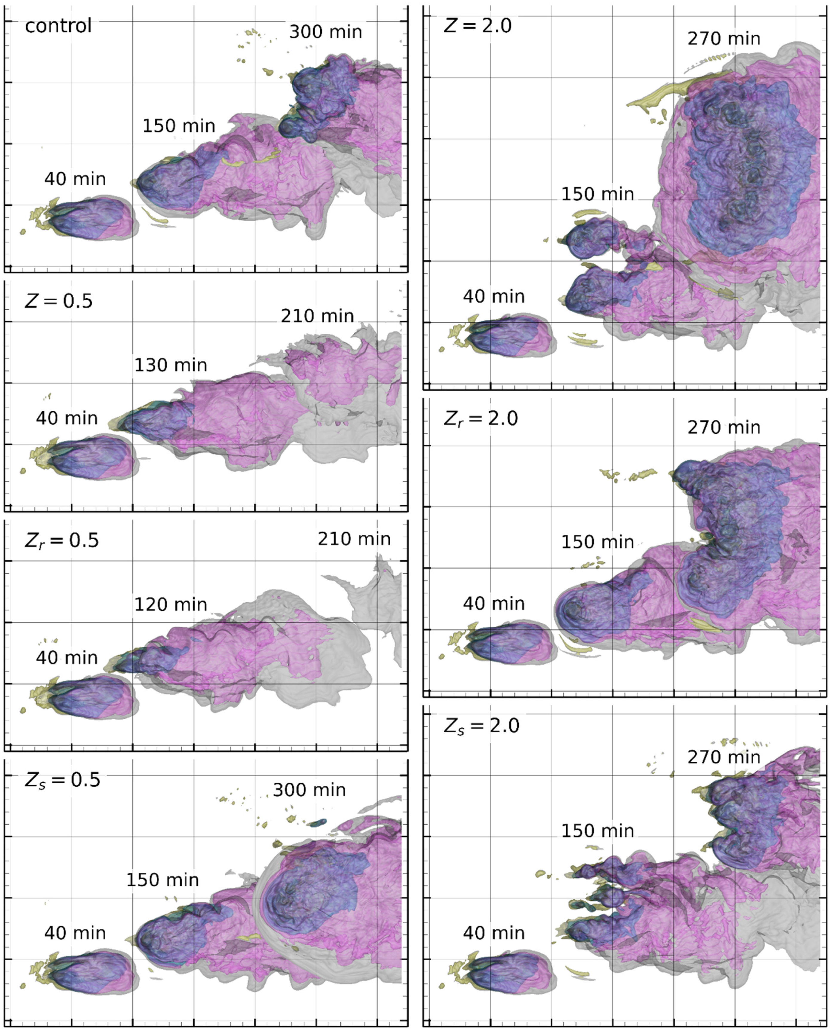
Figure 3 shows the top view of the simulated storms in all experiments at three suitably selected time steps to represent the early, mature, and later stages. The outermost surface of the storm is represented by the 0.1 g/kg (gray color) isosurface of the mixing ratio of total water condensates. The isosurfaces of the 0.1 g/kg mixing ratios of rain (yellow), snow (purple), and hail (blue) are also plotted.
In the control run, the storm lasts to the end of the simulation, when it splits into two cells. Before storm splitting, small cells emerge occasionally, but none of them grows large enough to affect the main cell. This differs from the control case of our previous study, where the storm dissipated at around 180 min. Reducing the ventilation effect of all three species together (Z = 0.5) results in early dissipation of the storm, whereas enhancing the ventilation (
) causes the storm to split and eventually evolve into a multicellular system. Despite the difference in the resulting lifespan compared with that in Chou et al.’s (2021) study [
20], the response of the storm’s development to changing ventilation parameterization agrees well with the earlier study.
Next, we will examine the cases where we reduce or enhance the ventilation separately for liquid and solid precipitation particles. Reducing the ventilation effect of only rain () causes earlier dissipation than reducing the ventilation of all species (). For these two cases, there is neither cell splitting nor new cell development in the simulation. On the contrary, enhancing the ventilation of rain () causes storm splitting and develops into multicellular structure, but with a smaller scale than in the case of . These two experiments on varying the ventilation effect of rain show that it could be a major factor affecting the storm’s development. The stronger the ventilation effect of rain, the stronger the storm will evolve into a larger system, and vice versa.
Varying the ventilation effect of snow and hail leads to more sophisticated consequences. Both reducing and enhancing the ventilation effect cause the storm to evolve into a larger-scale system than the control case, however, in distinct ways. In the case, although there is a small cell rising to the north of the cell at 210 min (not shown), it dissipates at the end (and its remnants could be seen to the north of the main cell), whereas the main storm remains intact. On the other hand, in the case of , the storm evolves with the characteristic new cell formation, splitting and merging. The appearance of a new cell occurs fairly early, at t = 80 min (not shown), and the storm evolves into a triplet at 150 min. These cells evolve independently of each other until t = 250 min, when they start to merge.
Examining the history of hydrometeor mass fluctuations provides clues as to possible mechanisms responsible for the storm’s evolutionary behavior as depicted in
Figure 3.
Figure 4 shows that all storm cases have nearly the same hydrometeor mass in each category up to
t ~ 70 min. In the
case, the mass of total condensates grows rapidly owing to the fast accumulating hail from 110 min (bottom panel) and of rain (middle panel) later from 150 min. It becomes the largest storm in terms of mass of rain, hail, and total water condensate at 150 min when it forms two firm cells (as shown in
Figure 3). Enhancing the ventilation effect of rain (
also causes the storm to grow substantially in mass but at a slower rate than
. Unlike
, it only produces one cell at 150 min, but with a round back-sheared anvil indicating strong divergent flow near the cloud top.
The case of enhancing the ventilation effect of snow and hail ( results in the production of a triplet system, yet its water condensate mass is the smallest during the mature stage among the four cases. The hail category contributes the most to losing the water condensate mass, likely due to the enhanced sublimation rate in the parameterization. The storm has grown rapidly in mass since 250 min ago, when cells started to merge.
On the other hand, in the case of decreasing the ventilation effect of snow and hail , the storm develops nearly linearly in terms of the mass of hail and total water condensates during the period between 120 and 240 min. The rise of the small cell mentioned previously is reflected by the faster increase of rain growth at 210 min, and of hail at 240 min. The dissipation of the small cell is, on the other hand, marked by the slowing down of hail and the total condensate mass growth rate at around 270 min.
Figure 5 shows the time series of the domain extrema of the vertical wind fields. These are smoothed curves that resulted from convolving with a discrete Gaussian kernel with a standard deviation of 4 min. The large fluctuations of the original curves (sampled every 2 min) make it difficult to identify the trends clearly, whereas it is much easier to do so by examining the smoothed curves.
A common feature of all the cases is that both the updraft/downdraft reach a peak between 50 and 60 min, followed by a sudden decline in magnitude. The peak occurs at about the same time as the overshooting top of the storm peaks for the first time. Many more fluctuations in maximum updraft/downdraft thereafter may follow, depending on the cases. We find that the large fluctuation occurs when the storm shows active intercellular processes, including frequent formation and dissipation of new cells, storm splitting, and cells merging. These intercellular processes often lead to multicellular complexes.
Inspection of the snapshots in the control run (not shown) reveals that the storm develops steadily before 180 min. Subsequently, new cells emerge vigorously to the north of the storm, followed by a splitting of the main cell at around 260 min. In this period (180–260 min), the maximum updrafts and downdrafts exhibit large fluctuations.
In the case, new cell formation and storm splitting occur frequently from 80 min to 150 min when it develops into two large cells. The extrema of vertical winds have larger fluctuations than the control run at this time. A triplet structure emerges at 180 min and a merged multicellular structure at 200 min (not shown). Although the storm changes morphology substantially, it grows steadily in size, and its vertical velocity extrema show less fluctuation than the early period.
In the case, there are vigorous new cell formation and splitting processes during the 80–250-min period, and the cells merge to form a multicellular system at around 270 min. However, the transformation is unsteady, and consequently, its vertical velocity extrema fluctuate more than the case throughout the simulation.
The steadiest case is where the storm evolves gradually into a single cell. Its extrema remain relatively constant at almost the highest values among all the experiments.
In the case, the storm grows steadily until 170 min, when a cell splits from the north of the main cell (not shown), which initiates a fast development into a multicellular cluster. However, the transformation is smoother than in the cases of the control run and . The extrema after the transformation show larger fluctuations than before but are still smaller than those in the same stage in the control run and cases.
The domain water condensate masses of all cases already show substantial differences in the 2nd hour, as seen in
Figure 4. The differences become even clearer when we examine the vertical distributions of precipitation particles, which suggest different paths in their developments. In
Figure 6, the total mass of rain and hail in each layer of the simulation domain is averaged over the period from 30 to 70 min, and the differences with respect to the control run are presented.
We see in
Figure 6 that enhancing the ventilation effect of rain (
, left panel) causes the rain mass to be smaller than the control run below the freezing level around 4 km but to be larger above the level. On the other hand, decreasing the ventilation effect of rain (
) results in the opposite trend. The role that the ventilation effect of rain plays in regulating condensation and evaporation, which have a direct impact on the mass gained and/or lost by rain, is clearly shown by these two cases.
Similarly, enhancing the ventilation effect of snow and hail (, right panel) results in more hail mass at levels between 6 and 12 km, and less hail mass below 6 km than in the control run. As is to , reducing the ventilation effect of snow/hail, (right panel), shows roughly the opposite trend to the case of .
Enhancing the ventilation effect of a specified category helps to enhance the vapor transport between the hydrometeor surface and the environmental air. The growth layer usually locates at higher levels, and the evaporation layer usually locates at lower levels. Hail forms at higher levels than rain, and the sublimation when falling through a subsaturated environment would undergo a longer distance than the evaporation of rain. Therefore, rain contributes more to gravitational fallout as a sink of water content in the storm than hail does. Reducing the ventilation effect of rain causes the evaporation rate to decrease, and the precipitation to increase as shown in the cases of and .
Reducing the ventilation effect of snow/hail slows down the sublimation, and the hail that falls below the freezing line would melt and form rain. In this case, rain undergoes a normal evaporation process, and the precipitation would be lighter than in the cases of and . This is likely one of the reasons that reducing the ventilation effect of rain would cause the storm to terminate earlier than the control run, but reducing the effect of snow/hail alone would not.
Adjusting the ventilation effects also has a direct impact on the thermal and dynamic processes of the storm because it impacts the rate of latent heat release or consumption. When evaporation/sublimation occur rapidly, the temperature of the surrounding air would become colder quickly, and downdrafts are stronger.
Figure 7 shows this effect. Here the updrafts/downdrafts averaged from 50 to 70 min with magnitudes greater than or equal to the 99.9 percentile on each level of domain are shown.
These top updrafts/downdrafts occupy about 10 × 10
of area. Below 5 km in height, the cases with enhanced ventilation effects have stronger downdrafts. The sublimation cooling has a stronger effect than the evaporative cooling. This is because (1) enhancing the ventilation effect of snow/hail produces more hail than the increase in rain produced by enhancing the rain ventilation, and (2) the latent heat absorbed is larger in sublimation than in evaporation. As a result, the case of
produces the strongest cooling and downdrafts, followed by the cases of
,
, and the control run, in that order, at levels below 5 km. The reduced ventilation cases show the opposite trend that
has stronger effect than
, followed by
, which has the smallest effect. Because the air is a continuum, when downdraft hits the ground level updraft will occur somewhere around the main storm cell and, if sufficiently strong, may even initiate new cells. The stronger downdrafts have a larger potential to generate greater updrafts than the weak ones. The updrafts in
Figure 7, below 4 km, show that their averaged magnitudes are arranged in the same order as the downdrafts.
The cases and have strongest updrafts on average at the early stage (50–70 min), where the storm becomes mature. In both cases, a strong updraft causes a new cell formation as early as 80 min, which grows to a size large enough to compete and interfere with the mother cell and other cells generated later. In the case of , although the cell grows steadily in size and lasts to the end, it has the second-weakest updrafts among all the cases. The weak updraft keeps the storm from remaining as a single cell as it evolves.
6. Conclusions
We performed an expanded set of sensitivity studies utilizing cloud model simulations to investigate how different ventilation parameterizations may impact the life span of the simulated storms. We used the widely adopted ventilation parameterizations as the control case and investigated the sensitivity of the reduced ventilation, normal, and enhanced ventilation effects by multiplying a constant factor ranging from 0.5 to 2.0 so as to represent the various degrees of enhancement.
Differing from our previous study (Chou et al., 2022) [
16], where the storm develops in a confined storm-following domain, our present study shows that the storm evolving freely in a larger domain lasts longer. This change in the lifespan is likely due to the effect of boundary conditions unrelated to ventilation sensitivity. However, it is worthy of note that the trends in the life span of the simulated storm in response to reducing/increasing the ventilation effects of all three hydrometeors are similar in the storm-following and fixed domain runs.
The impact of the ventilation effect on rain is the major factor affecting the lifespan of the storm. Modulating the ventilation effect of rain alone results in a similar trend as modulating the effect of all three species. Hail, on the other hand, controls the formation of new cells and the following intercellular processes. Increasing the ventilation effect of hail/snow increases cellular activity and the possibility of developing into a multicellular complex.
Despite the similarity in their appearance in the early mature stages, subtle discrepancies in the total hydrometeor masses and vertical wind fields among different cases reveal the effects caused by adjusting the ventilation coefficients, which lead to different paths of their further development.
Enhancing the ventilation effect of rain increases the rain’s evaporation rate below the freezing level and decreases the precipitation, and vice versa. On the other hand, enhancing the ventilation effect of snow/hail by increasing the rate of sublimation makes small differences in the total hail masses that fall to the surface in different cases. As an important sink of the total water content, which affects the storm lifespan, the gravitational fallout from rain dominates that from hail/snow. Hence, adjusting the ventilation effect of rain is a key factor affecting the lifespan of the storm.
On the other hand, although the hail/snow category affects less on the storm life span compared to rain, enhanced hail/snow ventilation still contributes to the adjustment of latent heat amount, which seems to be a factor leading to the multicellular structure.
This study thus demonstrates that the storm simulation results are sensitive to the parameterization of ventilation. It also demonstrated that a change in cloud microphysical parameters could lead to a large change in large-scale cloud behavior, such as the life span we investigated here.


