

Evolution over Time of Urban Thermal Conditions of a City Immersed in a Basin Geography and Mitigation


Abstract
:1. Introduction
1.1. Urban Densification
1.2. Mitigation Measures
2. Materials and Methods
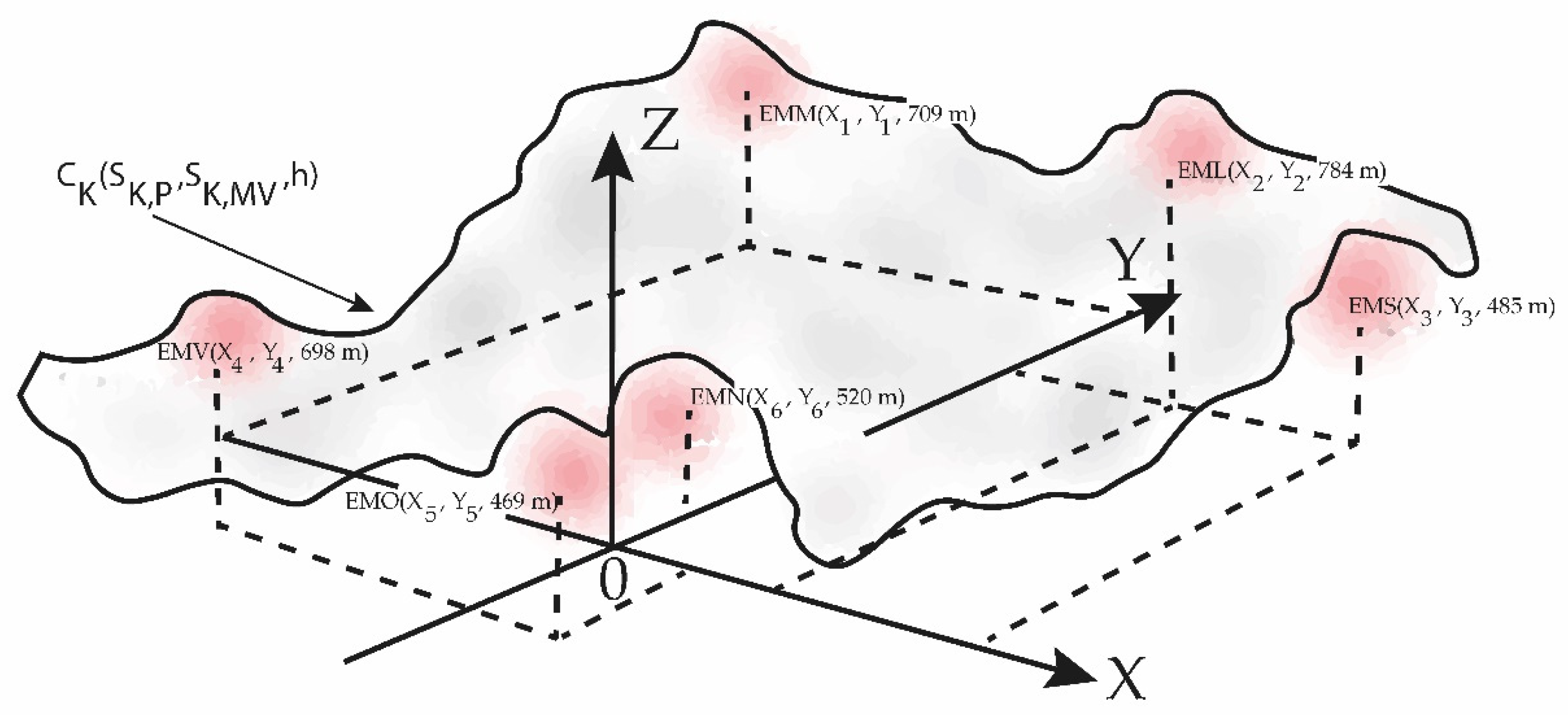
2.1. Measurement Recording Area
2.2. The Data
2.3. Kolmogorov Entropy and Loss Information
- (1).
- For each of the time series of the pollutants (P): PM10, PM2.5 and CO;
- (2).
- In the same way as in (1) for each meteorological variable (MV): temperature (T), magnitude of wind speed (WS) and relative humidity (RH) [3].
Flowchart
- The time series of meteorological variables and concentration of pollutants with many data [38] were measured hourly and simultaneously in all locations (6) used in the study.
- There can be no missing data in the time series. There are filling methods such as Kriging [39].
- As it is a procedure based on measurements, the quality of the measurement instruments is fundamental (certification and calibration, Environmental Protection Agency (EPA) [25]).
3. Results


4. Discussion
5. Conclusions
Author Contributions
Funding
Institutional Review Board Statement
Informed Consent Statement
Data Availability Statement
Acknowledgments
Conflicts of Interest
Appendix A

| Instrument | Pollutant | Responsible | Implementation |
|---|---|---|---|
| ADP | PM10, PM2.5, gases like SOx | MMA | In all Chile |
| SPMSR | PM30 | MGAP | Vallenar Province |
| AEIL19300 | PM10, PM2.5, gases like SOx, NOx, CHO | MMA, MINSAL, MGAP | In all Chile |
| SSRGP | PM10, PM2.5, gases like SOx, NOx, CHO | MINSAL | As primary regulation throughout Chile |
| CPA | Reducir GEI (Greenhouse effect gases) | MINECON, MMA, MINSAL | In all Chile |
| VR | PM10, PM2.5, gases like SOx, NOx, CHO | MINSAL | In localities of Chile with PDA |
| CFE | PM2.5, gases like SOx, NOx, CHO | MINSAL | In localities of Chile with PDA |
References
- Pacheco, P.R.; Salini, G.A.; Mera, E.M. Entropía y neguentropía: Una aproximación al proceso de difusión de contaminantes y su sostenibilidad. Rev. Int. Contam. Ambient. 2021, 37, 167–185. [Google Scholar] [CrossRef]
- Pacheco, P.; Mera, E.; Salini, G. Urban Densification Effect on Micrometeorology in Santiago, Chile: A Comparative Study Based on Chaos Theory. Sustainability 2022, 14, 2845. [Google Scholar] [CrossRef]
- Pacheco, P.; Mera, E. Relations between Urban Entropies, Geographical Configurations, Habitability and Sustainability. Atmosphere 2022, 13, 1639. [Google Scholar] [CrossRef]
- Pacheco, P.; Mera, E.; Fuentes, V.; Parodi, C. Initial Conditions and Resilience in the Atmospheric Boundary Layer of an Urban Basin. Atmosphere 2023, 14, 357. [Google Scholar] [CrossRef]
- Pacheco, P.; Mera, E.; Fuentes, V. Intensive Urbanization, Urban Meteorology and Air Pollutants: Effects on the Temperature of a City in a Basin Geography. Int. J. Environ. Res. Public Health 2023, 20, 3941. [Google Scholar] [CrossRef]
- INE-Plataforma de datos Estadísticos. 2020. Available online: https://www.ine.cl/docs/default-source/encuesta-suplementaria-deingresos/publicaciones-y-anuarios/sntesis-de-resultados/2019/sintesis-nacional-esi-2019.pdf (accessed on 1 December 2022).
- MVU—Ministerio de Vivienda y Urbanismo; y el Centro de Estudios de Ciudad y Territorio, (Housing and Urbanism Ministry and the Center for City and Territory Studies). 2020. Available online: https://observatoriourbano.minvu.gob.cl/estudios/ (accessed on 20 December 2022).
- Vergara, J.E. Verticalización. La edificación en altura en la región metropolitana de Santiago (1990–2014). Rev. INVI 2017, 32, 9–49. [Google Scholar] [CrossRef]
- PUBLICA. 2019. Available online: https://www.minvu.cl/wp-content/uploads/2019/06/CUENTA-PUBLICA-resumenejecutivo-2019-2.pdf (accessed on 8 January 2023).
- Stehr, N.; Von Storch, H. Introduction to papers on mitigation and adaptation strategies for climate change: Protecting nature from society or protecting society from nature? Environ. Sci. Policy 2005, 8, 537–540. [Google Scholar] [CrossRef]
- Stehr, N.; Von Storch, H. Adaptation and Mitigation and the Illusion of the Difference. GAIA—Ecol. Perspect. Sci. Soc. 2008, 17, 270–273. Available online: https://www.researchgate.net/publication/290922427 (accessed on 17 January 2023).
- Mirzaei, P.A.; Haghighat, F. Approaches to study urban heat island–abilities and limitations. Build. Environ. 2010, 45, 2192–2201. [Google Scholar] [CrossRef]
- Yuan, K.; Zhu, Q.; Riley, W.J.; Li, F.; Wu, H. Understanding and reducing the uncertainties of land surface energy flux partitioning within CMIP6 land models. Agric. For. Meteorol. 2022, 319, 108920. [Google Scholar] [CrossRef]
- Yuan, K.; Zhu, Q.; Zheng, S.; Zhao, L.; Chen, M.; Riley, W.J.; Cai, X.; Ma, H.; Li, M.; Wu, H. Deforestation reshapes land-surface energy-flux partitioning. Environ. Res. Lett. 2021, 16, 024014. [Google Scholar] [CrossRef]
- Balany, F.; Ng, A.W.; Muttil, N.; Muthukumaran, S.; Wong, M.S. Green Infrastructure as an Urban Heat Island Mitigation Strategy—A Review. Water 2020, 12, 3577. [Google Scholar] [CrossRef]
- Black, S.; Minnett, D.; Parry, I.; Roaf, J.; Zhunussova, K. A Framework for Comparing Climate Mitigation Effort across Countries; Working Paper 2022/254; International Monetary Fund: Washington, DC, USA, 2022. [Google Scholar]
- Fu, J.; Dupre, K.; Tavares, S.; King, D.; Banhalmi-Zakar, Z. Optimized greenery configuration to mitigate urban heat: A decade systematic review. Front. Archit. Res. 2022, 11, 466–491. [Google Scholar] [CrossRef]
- Yang, L.; Qian, F.; Song, D.-X.; Zheng, K.-J. Research on Urban Heat-island Effect. Procedia Eng. 2016, 169, 11–18. [Google Scholar] [CrossRef]
- Sun, Z.; Li, Z.; Zhong, J. Analysis of the Impact of Landscape Patterns on Urban Heat Islands: A Case Study of Chengdu, China. Int. J. Environ. Res. Public Health 2022, 19, 13297. [Google Scholar] [CrossRef]
- Palma Behnke, R.; Barría, C.; Basoa, K.; Benavente, D.; Benavides, C.; Campos, B.; de la Maza, N.; Farías, L.; Gallardo, L.; García, M.J.; et al. Chilean NDC Mitigation Proposal: Methodological Approach and Supporting Ambition; Mitigation and Energy Working Group Report; COP25 Scientific Committee; Ministry of Science, Technology, Knowledge and Innovation: Santiago, Chile, 2019. Available online: https://mma.gob.cl/wp-content/uploads/2020/03/Mitigation_NDC_White_Paper.pdf (accessed on 15 January 2023).
- Zhu, L.; Ge, X.; Chen, Y.; Zeng, X.; Pan, W.; Zhang, X.; Ben, S.; Yuan, Q.; Xin, J.; Shao, W.; et al. Short-term effects of ambient air pollution and childhood lower respiratory diseases. Sci. Rep. 2017, 7, 4414. [Google Scholar] [CrossRef]
- Martínez, J.A.; Vinagre, F.A. La Entropía de Kolmogorov; su Sentido Físico y su Aplicación al Estudio de Lechos Fluidizados 2D; Departamento de Química Analítica e Ingeniería Química, Universidad de Alcalá, Alcalá de Henares: Madrid, Spain, 2019; Available online: https://www.academia.edu/2479372/19/07/2019 (accessed on 23 September 2022).
- Shannon, C. A mathematical theory of communication. Bell Syst. Tech. 1948, 27, 379–423. [Google Scholar] [CrossRef]
- Rutland, J.; Garreaud, R. Meteorological air pollution for Santiago, Chile: Towards an objective episode forecasting. Environ. Monit. Assess. 1995, 34, 223–244. [Google Scholar] [CrossRef]
- MMA. Sistema de Información Nacional de Calidad del Aire. Ministerio del Medioambiente de Chile. 2020. Available online: https://sinca.mma.gob.cl/index.php (accessed on 9 January 2023).
- Farmer, J.D. Chaotic attractors of an infinite dimensional dynamical system. Phys. D 1982, 4, 366–393. [Google Scholar] [CrossRef]
- Farmer, J.D.; Otto, E.; Yorke, J.A. The dimension of chaotic attractors. Phys. D 1983, 7, 153–180. [Google Scholar] [CrossRef]
- Farmer, J.D. Information Dimension and the Probabilistic Structure of Chaos. Z. Nat. A 1982, 37, 1304–1326. [Google Scholar] [CrossRef]
- Kolmogorov, A.N. On Entropy per unit Time as a Metric Invariant of Automorphisms. Dokl. Akad. Nauk. SSSR 1959, 124, 754–755. [Google Scholar]
- Sinai, Y.G. On the concept of entropy of a dynamical system. Dolk. Akad. Nauk. SSSR 1959, 124, 768. [Google Scholar]
- Pesin, Y. Characteristic Lyapunov exponents and smooth ergodic theory. Russ. Math. Surv. 1977, 32, 55–114. [Google Scholar]
- Kolmogorov, A.N. A new invariant for transitive dynamical systems. Dokl. Akad. Nauk. Souiza Sovestkikh Sotsialisticheskikh Respuplik 1958, 119, 861–864. [Google Scholar]
- Ruelle, D. Thermodynamic Formalism; Addison-Wesley-Longman: Reading, MA, USA, 1978. [Google Scholar]
- Shaw, R. Strange aattractor, chaotic behavior, and information flow. Z. Nat. A 1981, 36, 80–112. [Google Scholar] [CrossRef]
- Abramson, N. Information Theory and Coding; McGraw-Hill: New York, NY, USA, 1963. [Google Scholar]
- Deco, G.; Schurmann, B. Information flow and chaotic dynamics. In Proceedings of the International Workshop on Neural Networks for Identification, Control, Robotics and Signal/Image Processing, Venice, Italy, 21–23 August 1996; IEEE: Venice, Italy, 1996; pp. 321–329. [Google Scholar] [CrossRef]
- Cohen, A.; Procaccia, I. Computing the Kolmogorov entropy from time signals of dissipative and conservative dynamical systems. Phys. Rev. A Gen. Phys. 1985, 31, 1872–1882. [Google Scholar] [CrossRef] [PubMed]
- Wolf, A.; Swift, J.B.; Swinney, H.L.; Vastano, J.A. Determining Lyapunov exponents from a time series. Phys. D 1985, 16, 285–317. [Google Scholar] [CrossRef]
- Emery, X. Simple and ordinary multigaussian Kriging for estimating recoverable reserves. Math. Geol. 2005, 37, 295–319. [Google Scholar] [CrossRef]
- Sprott, J.C. Chaos and Time-Series Analysis, 1st ed.; Oxford University Press: Oxford, UK, 2003. [Google Scholar]
- Sprott, J.C. Chaos Data Analyzer Software, Version 2.1; EEUU: Madison, WI, USA, 1995. Available online: https://sprott.physics.wisc.edu./cda.htm(accessed on 7 January 2023).
- Clausius, R. Über die bewegende Kraft der Wärme. Ann. Der Phys. 1850, 79, 368–397, 500–524. [Google Scholar] [CrossRef]
- Han, W.; Li, Z.; Wu, F.; Zhang, Y.; Guo, J.; Su, T.; Cribb, M.; Fan, J.; Chen, T.; Wei, J.; et al. The mechanisms and seasonal differences of the impact of aerosols on daytime surface urban heat island effect. Atmos. Chem. Phys. 2020, 20, 6479–6493. [Google Scholar] [CrossRef]
- Žiberna, I.; Pipenbaher, N.; Donša, D.; Škornik, S.; Kaligarič, M.; Bogataj, L.K.; Črepinšek, Z.; Grujić, V.J.; Ivajnšič, D. The Impact of Climate Change on Urban Thermal Environment Dynamics. Atmosphere 2021, 12, 1159. [Google Scholar] [CrossRef]
- United States Government. Available online: https://www.epa.gov/heatislands/climate-change-and-heat-islands (accessed on 10 January 2023).
- Pacheco, P.; Mera, E. Study of the Effect of Urban Densification and Micrometeorology on the Sustainability of a Coronavirus-Type Pandemic. Atmosphere 2022, 13, 1073. [Google Scholar] [CrossRef]
- Fahed, J.; Kinab, E.; Ginestet, S.; Adolphe, L. Impact of urban heat island mitigation measures on microclimate and pedestrian comfort in a dense urban district of Lebanon. Sustain. Cities Soc. 2020, 61, 102375. [Google Scholar] [CrossRef]
- Battista, G.; de Lieto Vollaro, E.; Ocłoń, P.; de Lieto Vollaro, R. Effects of urban heat island mitigation strategies in an urban square: A numerical modelling and experimental investigation. Energy Build. 2023, 282, 112809. [Google Scholar] [CrossRef]
- Songok, J.; Mäkiranta, A.; Rapantova, N.; Pospisil, P.; Martinkauppi, B. Numerical simulation of heat recovery from asphalt pavement in Finnish climate conditions. Int. J. Therm. Sci. 2023, 187, 108181. [Google Scholar] [CrossRef]
- Wen, J.; Ignatius, M.; Xinzhu Chen, E.; Hien Wong, N. Impacts of a highly reflective stainless-steel façade on a surrounding building: A case study in Singapore. Sustain. Cities Soc. 2023, 90, 104377. [Google Scholar] [CrossRef]
- Gourfi, A.; Taïbi, A.N.; Salhi, S.; Hannani, M.E.; Boujrouf, S. The Surface Urban Heat Island and Key Mitigation Factors in Arid Climate Cities, Case of Marrakesh, Morocco. Remote Sens. 2022, 14, 3935. [Google Scholar] [CrossRef]
- Park, C.; Ha, J.; Lee, S. Association between Three-Dimensional Built Environment and Urban Air Temperature: Seasonal and Temporal Differences. Sustainability 2017, 9, 1338. [Google Scholar] [CrossRef]
- Marsh, T.; Harvey, C.L. The Thames flood series: A lack of trend in flood magnitude and a decline in maximum levels. Hydrol. Res. 2012, 43, 203–214. [Google Scholar] [CrossRef]
- Coman, I.A.; Cooper-Norris, C.E.; Longing, S.; Perry, G. It Is a Wild World in the City: Urban Wildlife Conservation and Communication in the Age of COVID-19. Diversity 2022, 14, 539. [Google Scholar] [CrossRef]
- Murray, M.H.; Byers, K.A.; Buckley, J.; Lehrer, E.W.; Kay, C.; Fidino, M.; Magle, S.B.; German, D. Public perception of urban wildlife during a COVID-19 stay-at-home quarantine order in Chicago. Urban Ecosyst. 2023, 26, 127–140. [Google Scholar] [CrossRef] [PubMed]
- Perez, P.; Salini, G. A Study of the Dynamic Behaviour of Fine Particulate Matter in Santiago, Chile. Aerosol Air Qual. Res. 2015, 15, 154–165. [Google Scholar] [CrossRef]
- Hu, H.; Tan, Z.; Liu, C.; Wang, Z.; Cai, X.; Wang, X.; Ye, Z.; Zheng, S. Multi-timescale analysis of air pollution spreaders in Chinese cities based on a transfer entropy network. Front. Environ. Sci. 2022, 10, 970267. [Google Scholar] [CrossRef]


| Station Name | Location | PM10 | PM2.5 | CO | T | RH | WV | OWNER |
|---|---|---|---|---|---|---|---|---|
| 1. La Florida, EML, masl:784 m | 33°30′59.7′′ S 70°35′17.4′′ W | Attenuation Beta-Met One 1020 | Attenuation Beta-Met One 1020 | Gas Correlation Filter IR Photometry -Thermo 48i | VAISALA HMP35A | VAISALA HMP35A | Sensor-Met One 010C | SINCA |
| 2. Las Condes, EMM, masl:709 m | 33°22′35.8′′ S 70°31′23.6′′ W | Attenuation Beta-Met One 1020 | Attenuation Beta-Met One 1020 | Gas Correlation Filter IR Photometry -Thermo 48i | VAISALA HMP35A | VAISALA HMP35A | Sensor-Met One 010C | SINCA |
| 3. Santiago- Parque O’Higgins, EMN, masl: 570 m | 33°27′50.5′′ S 70°39′38.5′′ W | Attenuation Beta-Met One 1020 | Attenuation Beta-Met One 1020 | Gas Correlation Filter IR Photometry -Thermo 48i | VAISALA HMP35A | VAISALA HMP35A | Sensor-Met One 010C | SINCA |
| 4. Pudahuel, EMO, masl:469 m | 33°27′06.2′′ S 70°40′07.8′′ W | Attenuation Beta-Met One 1020 | Attenuation Beta-Met One 1020 | Gas Correlation Filter IR Photometry -Thermo 48i | VAISALA HMP35A | VAISALA HMP35A | Sensor-Met One 010C | SINCA |
| 5. Puente Alto, EMS, masl:698 m | 33°33′01.3′′ S 70°34′51.4′′ W | Attenuation Beta-Met One 1020 | Attenuation Beta-Met One 1020 | Gas Correlation Filter IR Photometry -Thermo 48i | VAISALA HMP35A | VAISALA HMP35A | Sensor-Met One 010C | SINCA |
| 6. Quilicura, EMV, masl:485 m | 33°21′51.6′′ S 70°44′53.9′′ W | Oscillating Element Microbalance TEOM-Thermo 1400AB | Attenuation Beta-Met One 1020 | Gas Correlation Filter IR Photometry -Thermo 48i | VAISALA HMP35A | VAISALA HMP35A | Sensor-Met One 010C | SINCA |
| Parameters Station | PM10 (µg/m3) | PM2.5 (µg/m3) | CO (ppm) | Temperature (°C) | HR (%) | WV (m/s) |
|---|---|---|---|---|---|---|
| EML | ||||||
| λ | 0.716 0.031 | 0.246 0.020 | 0.025 0.007 | 0.191 0.016 | 0.167 0.017 | 0.314 0.016 |
| Dc | 1.067 0.203 | 1.306 0.172 | 2.089 0.052 | 1.632 0.798 | 2.465 0.701 | 1.991 0.045 |
| H | 0.930 | 0.946 | 0.933 | 0.920 | 0.934 | 0.942 |
| SK (1/h) | 0.257 | 0.367 | 0.382 | 0.175 | 0.229 | 0.275 |
| LZ | 0.164 | 0.257 | 0.0164 | 0.073 | 0.144 | 0.181 |
| EMM | ||||||
| λ | 0.561 0.028 | 0.345 0.022 | 0.011 0.006 | 0.220 0.016 | 0.203 0.018 | 0.339 0.016 |
| Dc | 0.984 0.071 | 1.531 0.359 | 2.156 0.006 | 1.923 0.781 | 2.691 0.683 | 1.986 0.071 |
| H | 0.914 | 0.969 | 0.933 | 0.916 | 0.935 | 0.942 |
| SK (1/h) | 0.247 | 0.360 | 0.333 | 0.182 | 0.180 | 0.278 |
| LZ | 0.117 | 0.382 | 0.0084 | 0.080 | 0.111 | 0.176 |
| EMN | ||||||
| λ | 0.727 0.031 | 0.242 0.020 | 0.026 0.007 | 0.184 0.015 | 0.060 0.011 | 0.328 0.016 |
| Dc | 0.978 0.049 | 1.421 0.262 | 2.053 0.019 | 1.626 0.813 | 2.752 0.629 | 1.997 0.073 |
| H | 0.934 | 0.947 | 0.933 | 0.921 | 0.908 | 0.941 |
| SK (1/h) | 0.409 | 0.385 | 0.333 | 0.172 | 0.148 | 0.283 |
| LZ | 0.205 | 0.312 | 0.018 | 0.062 | 0.086 | 0.182 |
| EMO | ||||||
| λ | 0.540 0.027 | 0.332 0.022 | 0.015 0.006 | 0.222 0.016 | 0.256 0.020 | 0.347 0.016 |
| Dc | 0.973 0.059 | 1.354 0.225 | 2.095 0.075 | 1.821 0.708 | 2.499 0.598 | 2.019 0.077 |
| H | 0.940 | 0.920 | 0.933 | 0.918 | 0.936 | 0.941 |
| SK (1/h) | 0.388 | 0.400 | 0.329 | 0.180 | 0.205 | 0.283 |
| LZ | 0.183 | 0.326 | 0.012 | 0.069 | 0.126 | 0.182 |
| EMS | ||||||
| λ | 0.747 0.032 | 0.257 0.020 | 0.021 0.007 | 0.194 0.015 | 0.104 0.14 | 0.349 0.016 |
| Dc | 0.940 0.028 | 1.232 0.118 | 1.883 0.194 | 1.662 0.810 | 2.770 0.701 | 2.005 0.050 |
| H | 0.930 | 0.964 | 0.933 | 0.919 | 0.930 | 0.942 |
| SK (1/h) | 0.280 | 0.346 | 0.404 | 0.168 | 0.149 | 0.290 |
| LZ | 0.204 | 0.252 | 0.012 | 0.068 | 0.085 | 0.182 |
| EMV | ||||||
| λ | 0.574 0.030 | 0.241 0.021 | 0.580 0.077 | 0.161 0.014 | 0.714 0.048 | 0.080 0.013 |
| Dc | 0.945 0.017 | 1.432 0.216 | 2.127 0.110 | 1.559 0.761 | 2.704 0.036 | 1.939 0.078 |
| H | 0.930 | 0.938 | 0.933 | 0.920 | 0.934 | 0.940 |
| SK (1/h) | 0.252 | 0.415 | 0.285 | 0.153 | 0.100 | 0.351 |
| LZ | 0.175 | 0.337 | 0.0014 | 0.054 | 0.027 | 0.165 |
| h (masl) | 2010–2013 | 2017–2020 | 2019–2022 | % Variation | % Variation | % Variation |
|---|---|---|---|---|---|---|
| CK1 (Series 1) | CK2 (Series 2) | CK3 (Series 3) | 1-CK2/CK1 | 1-CK3/CK1 | 1-CK3/CK2 | |
| 784 (EML) | 0.865 | 0.814 | 0.675 | 6.0 | 22.0 | 17.1 |
| 709 (EMM) | 0.937 | 0.857 | 0.680 | 8.5 | 27.4 | 21.0 |
| 698 (EMS) | 0.936 | 0.734 | 0.589 | 22.0 | 37.0 | 20.0 |
| 570 (EMN) | 0.824 | 0.774 | 0.535 | 6.1 | 35.0 | 31.0 |
| 485 (EMV) | 0.834 | 0.815 | 0.635 | 2.3 | 26.0 | 24.0 |
| 469 (EMO) | 0.989 | 0.609 | 0.598 | 38.0 | 40.0 | 2.0 |
| 2010–2013 | 2017–2020 | 2019–2022 | ||
|---|---|---|---|---|
| Station | h (m) | Series 1 | Series 2 | Series 3 |
| EML (La Florida) | 784 | 0.865 | 0.814 | 0.675 |
| EMM (Las Condes) | 709 | 0.937 | 0.857 | 0.680 |
| EMV (Quilicura) | 485 | 0.834 | 0.815 | 0.635 |
| EMN (Santiago) | 570 | 0.824 | 0.774 | 0.535 |
| EMS (Puente Alto) | 698 | 0.936 | 0.734 | 0.589 |
| EMO (Pudahuel) | 469 | 0.989 | 0.609 | 0.598 |
| Stations | EML | EMM | EMN | EMO | EMS | EMV |
|---|---|---|---|---|---|---|
| Periods | <ΔI>P; <ΔI>MV | <ΔI>P; <ΔI>MV | <ΔI>P; <ΔI>MV | <ΔI>P; <ΔI>MV | <ΔI>P; <ΔI>MV | <ΔI>P; <ΔI>MV |
| 2010–2013 | −5.341; −6.079 | −5.039; −6.859 | −4.537; −6.357 | −3.271; −6.633 | −4.656; −6.955 | −3.825; −6.899 |
| 2017–2020 | −2.694; −4.000 | −3.355; −3.957 | −3.142; −4.092 | −3.083; −3.980 | −3.010; −4.066 | −2.827; −3.820 |
| 2019–2022 | −3.278; −2.232 | −3.046; −2.531 | −3.305; −1.900 | −2.946; −2.741 | −3.405; −2.149 | −4.634; −3.172 |
| EML | EMM | EMV | EMN | EMS | EMO | Average by Commune | |
|---|---|---|---|---|---|---|---|
| 2010–2013 | |||||||
| (°C) | 15.4 | 15.86 | 15.80 | 15.34 | 14.70 | 16.80 | 15.65 |
| (%) | 58.20 | 58.13 | 57.34 | 60.22 | 60.07 | 57.52 | 58.58 |
| 2017–2020 | |||||||
| (°C) | 16.12 | 15.57 | 16.85 | 16.17 | 15.53 | 16.78 | 16.17 |
| (%) | 55.31 | 55.00 | 58.95 | 57.31 | 56.07 | 59.22 | 56.98 |
| 2019–2022 | |||||||
| (°C) | 16.10 | 14.70 | 15.50 | 16.05 | 15.42 | 15.31 | 15.51 |
| (%) | 56.20 | 57.83 | 61.20 | 60.84 | 56.96 | 61.32 | 59.10 |
| PM10 | PM2.5 | CO | T | HR | WV | ||
|---|---|---|---|---|---|---|---|
| EML | 2010–2013 | ||||||
| H | 0.967 | 0.973 | 0.959 | 0.989 | 0.991 | 0.976 | |
| D | 1.033 | 1.027 | 1.041 | 1.011 | 1.009 | 1.024 | |
| 2017–2020 | |||||||
| H | 0.922 | 0.963 | 0.933 | 0.915 | 0.942 | 0.975 | |
| D | 1.078 | 1.037 | 1.067 | 1.085 | 1.058 | 1.025 | |
| 2019–2022 | |||||||
| H | 0.928 | 0.946 | 0.933 | 0.920 | 0.934 | 0.942 | |
| D | 1.072 | 1.054 | 1.067 | 1.080 | 1.066 | 1.058 | |
| EMM | 2010–2013 | ||||||
| H | 0.972 | 0.977 | 0.981 | 0.991 | 0.990 | 0.980 | |
| D | 1.028 | 1.023 | 1.019 | 1.009 | 1.010 | 1.02 | |
| 2017–2020 | |||||||
| H | 0.906 | 0.983 | 0.933 | 0.917 | 0.941 | 0.976 | |
| D | 1.094 | 1.017 | 1.067 | 1.083 | 1.059 | 1.024 | |
| 2019–2022 | |||||||
| H | 0.914 | 0.969 | 0.933 | 0.916 | 0.935 | 0.942 | |
| D | 1.086 | 1.031 | 1.067 | 1.084 | 1.065 | 1.058 | |
| EMN | 2010–2013 | ||||||
| H | 0.972 | 0.974 | 0.953 | 0.989 | 0.991 | 0.968 | |
| D | 1.028 | 1.026 | 1.047 | 1.011 | 1.009 | 1.032 | |
| 2017–2020 | |||||||
| H | 0.929 | 0.960 | 0.933 | 0.916 | 0.942 | 0.973 | |
| D | 1.071 | 1.040 | 1.067 | 1.084 | 1.058 | 1.027 | |
| 2019–2022 | |||||||
| H | 0.934 | 0.947 | 0.933 | 0.921 | 0.908 | 0.941 | |
| D | 1.066 | 1.053 | 1.067 | 1.079 | 1.092 | 1.059 | |
| EMO | 2010–2013 | ||||||
| H | 0.965 | 0.955 | 0.937 | 0.992 | 0.989 | 0.968 | |
| D | 1.035 | 1.045 | 1.063 | 1.008 | 1.011 | 1.032 | |
| 2017–2020 | |||||||
| H | 0.936 | 0.925 | 0.933 | 0.919 | 0.942 | 0.974 | |
| D | 1.064 | 1.075 | 1.067 | 1.081 | 1.058 | 1.026 | |
| 2019–2022 | |||||||
| H | 0.938 | 0.915 | 0.933 | 0.918 | 0.936 | 0.941 | |
| D | 1.062 | 1.085 | 1.067 | 1.082 | 1.064 | 1.059 | |
| EMS | 2010–2013 | ||||||
| H | 0.969 | 0.973 | 0.953 | 0.990 | 0.992 | 0.957 | |
| D | 1.031 | 1.027 | 1.047 | 1.010 | 1.008 | 1.043 | |
| 2017–2020 | |||||||
| H | 0.921 | 0.975 | 0.933 | 0.915 | 0.942 | 0.976 | |
| D | 1.079 | 1.025 | 1.067 | 1.085 | 1.058 | 1.024 | |
| 2019–2022 | |||||||
| H | 0.930 | 0.964 | 0.933 | 0.919 | 0.927 | 0.942 | |
| D | 1.070 | 1.036 | 1.067 | 1.081 | 1.073 | 1.058 | |
| EMV | 2010–2013 | ||||||
| H | 0.967 | 0.970 | 0.952 | 0.989 | 0.989 | 0.956 | |
| D | 1.033 | 1.03 | 1.048 | 1.011 | 1.011 | 1.044 | |
| 2017–2020 | |||||||
| H | 0.931 | 0.966 | 0.933 | 0.919 | 0.942 | 0.975 | |
| D | 1.069 | 1.034 | 1.067 | 1.081 | 1.058 | 1.025 | |
| 2019–2022 | |||||||
| H | 0.930 | 0.938 | 0.933 | 0.920 | 0.934 | 0.940 | |
| D | 1.070 | 1.062 | 1.067 | 1.080 | 1.066 | 1.060 | |
| h (masl) | (°C) | SK,P (1/h) | SK,MV (1/h) | (δQ/dt)P (K/h) | (δQ/dt)MV (K/h) | Δ (K/h) |
|---|---|---|---|---|---|---|
| 784 (EML) | 16.10 | 1.006 | 0.679 | 280.9855 | 196.4007 | 84.5848 |
| 709 (EMM) | 14.70 | 0.940 | 0.640 | 270.5790 | 184.2240 | 86.3550 |
| 698 (EMV) | 15.50 | 0.952 | 0.604 | 274.7948 | 174.3446 | 100.4502 |
| 520 (EMN) | 16.05 | 1.127 | 0.603 | 325.9284 | 174.3876 | 151.5408 |
| 485 (EMS) | 15.42 | 1.030 | 0.607 | 297.2271 | 175.1620 | 122.0651 |
| 469 (EMO) | 15.31 | 1.117 | 0.668 | 322.2098 | 192.6913 | 129.5185 |
| 15.51 | 295.2874 | 182.8684 | 112.4190 |
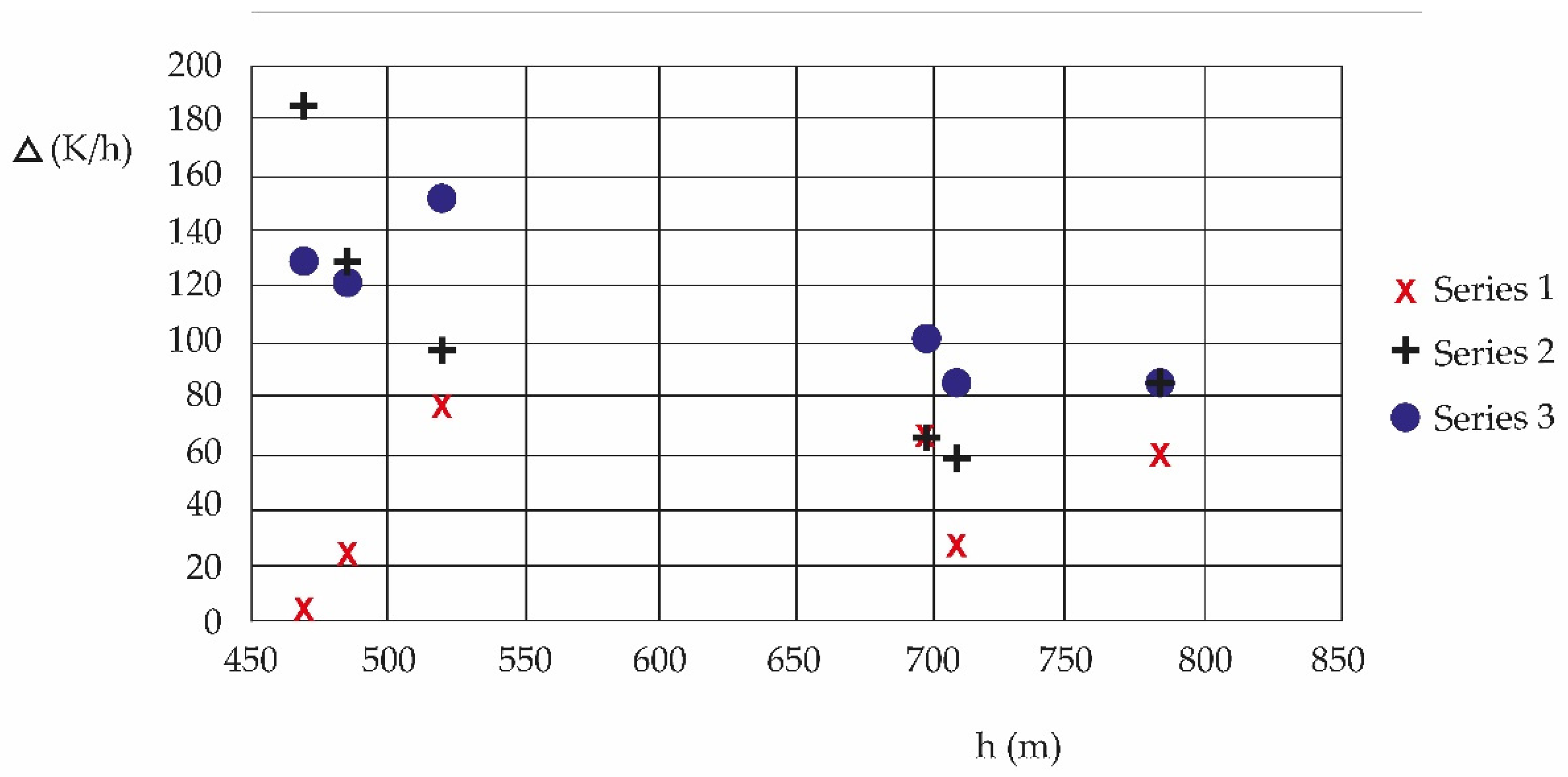
| 2010–2013 | 2017–2020 | 2019–2022 | |
|---|---|---|---|
| h (m) | Δ (Series 1) | Δ (Series 2) | Δ (Series 3) |
| 784 | 60.02 | 84.7561 | 84.5848 |
| 709 | 28.00 | 58.0327 | 86.3550 |
| 698 | 66.10 | 65.5400 | 100.4502 |
| 520 | 78.00 | 96.6329 | 151.5408 |
| 485 | 25.33 | 130.4833 | 122.0651 |
| 469 | 3.80 | 184.6982 | 129.5185 |
Disclaimer/Publisher’s Note: The statements, opinions and data contained in all publications are solely those of the individual author(s) and contributor(s) and not of MDPI and/or the editor(s). MDPI and/or the editor(s) disclaim responsibility for any injury to people or property resulting from any ideas, methods, instructions or products referred to in the content. |
© 2023 by the authors. Licensee MDPI, Basel, Switzerland. This article is an open access article distributed under the terms and conditions of the Creative Commons Attribution (CC BY) license (https://creativecommons.org/licenses/by/4.0/).
Share and Cite
Pacheco, P.; Mera, E. Evolution over Time of Urban Thermal Conditions of a City Immersed in a Basin Geography and Mitigation. Atmosphere 2023, 14, 777. https://doi.org/10.3390/atmos14050777
Pacheco P, Mera E. Evolution over Time of Urban Thermal Conditions of a City Immersed in a Basin Geography and Mitigation. Atmosphere. 2023; 14(5):777. https://doi.org/10.3390/atmos14050777
Chicago/Turabian StylePacheco, Patricio, and Eduardo Mera. 2023. "Evolution over Time of Urban Thermal Conditions of a City Immersed in a Basin Geography and Mitigation" Atmosphere 14, no. 5: 777. https://doi.org/10.3390/atmos14050777