Article

Use of Assimilation Analysis in 4D-Var Source Inversion: Observing System Simulation Experiments (OSSEs) with GOSAT Methane and Hemispheric CMAQ

1
Department of Civil and Environmental Engineering, Carleton University, Ottawa, ON K1S 5B6, Canada
2
Air Quality Research Division, Environment and Climate Change Canada, Dorval, QC H9P 1J3, Canada
3
Department of Physics, University of Toronto, Toronto, ON M5S 1A7, Canada
*
Author to whom correspondence should be addressed.
Atmosphere 2023, 14(4), 758; https://doi.org/10.3390/atmos14040758
Submission received: 13 March 2023 / Revised: 14 April 2023 / Accepted: 16 April 2023 / Published: 21 April 2023
(This article belongs to the Section Atmospheric Techniques, Instruments, and Modeling)

Abstract

:
We previously introduced the parametric variance Kalman filter (PvKF) assimilation as a cost-efficient system to estimate the dynamics of methane analysis concentrations. As an extension of our development, this study demonstrates the linking of PvKF to a 4D-Var inversion aiming to improve on methane emissions estimation in comparison with the traditional 4D-Var. Using the proposed assimilation–inversion framework, we revisit fundamental assumptions of the perfect and already optimal model state that is typically made in the 4D-Var inversion algorithm. In addition, the new system objectively accounts for error correlations and the evolution of analysis error variances, which are non-trivial or computationally prohibitive to maintain otherwise. We perform observing system simulation experiments (OSSEs) aiming to isolate and explore various effects of the assimilation analysis on the source inversion. The effect of the initial field of analysis, forecast of analysis error covariance, and model error is examined through modified 4D-Var cost functions, while different types of perturbations of the prior emissions are considered. Our results show that using PvKF optimal analysis instead of the model forecast to initialize the inversion improves posterior emissions estimate (~35% reduction in the normalized mean bias, NMB) across the domain. The propagation of analysis error variance using the PvKF formulation also tends to retain the effect of background correlation structures within the observation space and, thus, results in a more reliable estimate of the posterior emissions in most cases (~50% reduction in the normalized mean error, NME). Our sectoral analysis of four main emission categories indicates how the additional information of assimilation analysis enhances the constraints of each emissions sector. Lastly, we found that adding the PvKF optimal analysis field to the cost function benefits the 4D-Var inversion by reducing its computational time (~65%), while including only the error covariance in the cost function has a negligible impact on the inversion time (10–20% reduction).

1. Introduction

Methane (CH4) is a critical atmospheric component in both climate and air-quality contexts [1]. Over the past decade, a continuous increase in global methane concentrations has drawn urgent attention to quantifying and reducing methane emissions [2,3,4,5]. Methane emissions are derived from either the bottom-up or top-down estimation methods. Despite containing a substantial amount of data, bottom-up inventories suffer from two weaknesses: (i) significant uncertainties, due to inaccurate or missing information and (ii) not being constrained by atmospheric observations to retain a closed-form global budget [2,6,7]. Those eventually can hinder progress toward methane mitigation policies [8]. Top-down inventories, also known as atmospheric inversion, are less prone to issues of the bottom-up method due to incorporating information from observations. In particular, observations and a chemical transport model (CTM) are used together to make corrections to the prior bottom-up emissions. Providing adequate information from the observation network along with an accurate CTM maintains a top-down estimation that is less dependent on the prior emissions, resulting in estimated emissions with lower uncertainties. Satellite observations have been extensively used over the past decades to infer methane emissions on different scales, due to their higher density and global spatial coverage [9,10].
Atmospheric inversions play a key role in evaluating and improving bottom-up estimation but carry their own limitations for constraining methane emissions. For example, global and regional inversions are usually incapable of resolving emissions of small source sectors, such as non-wetland emissions, due to their minimal sensitivity to atmospheric observations [2,11]. Inversions can also depend on the choice of the prior emissions, particularly over areas where the observation constraints are limited or observations are not precisely determined [12,13]. In addition, significant uncertainties in the inversion are attributed to satellite measurements. Previous studies indicated a large discrepancy between satellite retrievals (e.g., from Scanning Imaging Absorption Spectrometer for Atmospheric Chartography, SCIAMACHY) and in situ measurements [14,15,16]. Furthermore, inversions rely on a CTM to translate the emissions signal into the observation space. Although advancements in remote sensing and emissions inventories every year provide us with more accurate satellite measurements and more reliable prior emissions, potential errors in CTM still exist and may reflect on the inversion results [17,18].
Many earlier methane inversion studies assume that the CTM is perfect [19,20,21,22]. However, it has been shown that running inversion with different CTMs can exert a tangible discrepancy in emissions estimates [18,23]. Transport errors such as those originating from meteorological fields, model advection parameterization, and model spatial and temporal resolutions are identified as crucial aspects contributing to the CTM’s error, particularly on a short timescale [18,24,25,26]. One promising way to address those errors is to simultaneously estimate emissions and model errors, such as through weak-constraint 4D-Var [25,27,28]. However, besides substantial computational cost, such a method applied to methane estimation does not account for the entire model error in the state, as the errors may not necessarily originate due to transport [29,30]. For example, errors in the chemistry, initial, and boundary conditions are among those that may not be addressed through methane weak-constraint 4D-Var.
A reliable emissions inversion result depends on maintaining a precise and realistic state estimation, whether it is used as the initial state (or background) or boundary conditions in a limited domain. One way to fulfill that requirement is to jointly estimate the state and source [31]. A joint estimation typically entails a substantial extra computational cost mainly due to resolving posterior errors for both concentrations and emissions. Furthermore, the procedure may not lead to a convergence of emissions [15]. This is likely due to the fact that the impact of the initial or boundary conditions on methane concentrations is much larger than the emissions, although with less variability. From an estimation point of view, the emissions signal in the inversion is masked by a larger influence of the (inflow or initial) concentrations. Thus, a joint estimation entails reducing the state uncertainties to a level comparable to or lower than the emissions signal, which is hardly achievable.
Chemical data assimilation may be used to separately estimate the model state concentrations and its error statistics. It is a promising method that is also used to deal with the issue of the state in inverse modelling. Previous studies assumed that the initial (or boundary) concentrations provided by the model or assimilation system are perfectly known; hence, potential uncertainties from the state cannot be taken into account for performing an inversion [32,33]. On the other hand, obtaining the state and its error statistics objectively using conventional data assimilation approaches, such as 4D-Var and EnKF assimilations, is a task with high computational cost [34,35,36,37]. Arguably, the core of data assimilation and inverse modelling lies in robust and objective quantifications of errors. We use a different assimilation system known as the parametric variance Kalman filter (PvKF), which is designed to provide a near-optimal methane analysis and its realistic error variance estimates [38]. For state estimation, PvKF is computationally more advantageous than EnKF and 4D-Var, such that it requires an equivalent cost of only two model integrations [34]. However, unlike the two other systems, PvKF assimilation itself is yet to be capable of performing source estimation.
The main objective of this study is to determine whether and how methane assimilated concentrations (i.e., optimal state analysis) and their estimated error statistics can improve on methane emissions estimations. To answer these questions, we frame a new source estimation system that links PvKF assimilation to a 4D-Var inversion technique. Figure 1 shows the schematic view of this problem with the main elements involved. One major focus of this assimilation–inversion framework is to evaluate the contribution of the state concentrations estimation for constraining methane emissions. Accordingly, not only can we change the first-guess concentrations to the cost function, but also explicitly include the estimate of error covariances of assimilation analysis for performing a source inversion. Besides the computational efficiency, PvKF formulation allows for dynamically propagating the errors while not relying on a perfect model assumption ( ϵ q 0 ). The modified formulation also accounts for model spatial correlation structures during the inversion, which is typically missed in methane inversion studies that simply rely on diagonal observation error covariance matrices [13,25,30,39,40,41,42,43]. Altogether, previous methane inversion studies are based on a set of questionable assumptions, which are challenged using our proposed approach in this study. Those assumptions include (i) perfect initial state concentrations and (ii) not propagating those errors throughout the inversion, and (iii) a perfect model (i.e., no modelling error).
To verify the ability of our framework, we conduct observing system simulation experiments (OSSEs) using the hemispheric Community Multiscale Air Quality (CMAQ) [44] model and simulate Greenhouse Gases Observing Satellite (GOSAT) observations. Our inversions optimize monthly mean methane emissions while three major anthropogenic and one natural category of methane emissions categories are considered. Using different initial conditions and modified formulations of a 4D-Var cost function, we are able to determine three different assimilation effects on the source inversion, including (i) the effect of the optimal initial analysis field, (ii) the model-propagated analysis error covariance, and (iii) the approximated model error. We perform different perturbations of the prior methane emissions, aiming to address the limitation of a typical 4D-Var inversion that relies on perfect state assumptions (i.e., initial and CTM) as well as a diagonal observation error covariance. In addition, the impacts of those cost-function configurations on the inversion of individual source sectors are further demonstrated in our analyses.

2. Methodology

4D-Var methane inversions in the past mainly assumed that the initial state concentrations were perfectly known [12,33,45,46,47]; in addition, a perfect CTM to simulate the methane in the atmosphere was typically taken into account. In both cases, the uncertainty of the state is considered to be negligible; therefore, it does not play a role in the inversion process. Although for an extended period of model integration (e.g., six months and more), those assumptions might be acceptable due to the homogeneity of the background methane concentrations [42], the errors in the state, such as transport error, for a short period of inversion (e.g., one month) are considerable and thus can exert a large impact on source estimation [25]. Accordingly, in order to proceed to more temporally resolved emissions inversions, an advancement in methodology is required that accounts for the errors in the state concentration level.
Our approach is composed of two main parts. First, we perform an assimilation of CH4 observations using the PvKF framework in order to provide a first-guess concentration field along with the error variance of the concentrations. Then, the second part executes a source inversion using a 4D-Var cost function with a modified error covariance weight that accounts for both observation errors and model-propagated errors. In other words, we seek to examine the capability of an alternative 4D-Var inversion formalism, which not only depends on the initial field and its corresponding error variance field but also relies on the model-propagated uncertainties and the approximated model errors. An illustration of how the PvKF assimilation framework is linked to a 4D-Var inversion system in order to address the effects of those state characteristics on methane source estimation is provided later in Figure 1 and throughout Section 2.4. Before that, in this section, an overview of GOSAT observations, the CMAQ model, and the prior emissions used in both PvKF and 4D-Var systems are presented as follows.

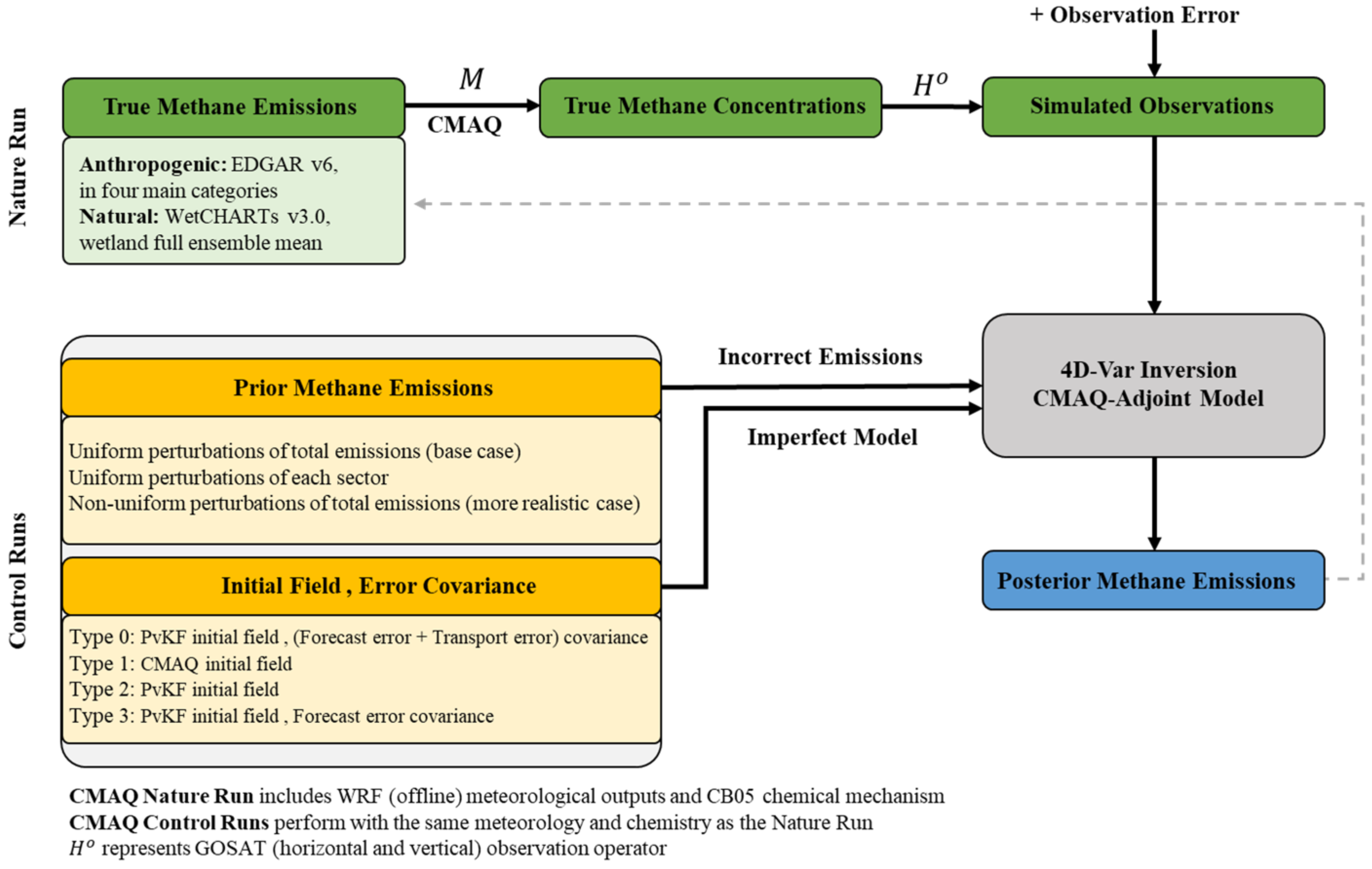
2.1. Satellite and Pseudo Observations

GOSAT, launched in January 2009 by the Japanese Space Agency (JAXA) [48], is in a Sun-synchronous orbit at an altitude of 666 km with a 3-day revisit time. The primary goal of GOSAT is to monitor the abundance of greenhouse gas, including atmospheric methane, globally. Because of the instrument’s global coverage, reasonable spatiotemporal resolution, and acceptable near-surface sensitivities, the assimilation of methane and inverse modelling of its sources and sinks using GOSAT observations is desirable. GOSAT retrievals provide a column-average dry-mole fraction of methane that corresponds to the methane average volume mixing ratio (VMR) of a partial column atmosphere. Methane VMRs and the corresponding standard deviations are obtained by performing a retrieval algorithm on the radiance spectrum. We use GOSAT proxy products from the retrieval algorithm developed at the Netherlands Institute for Space Research (SRON) and Karlsruhe Institute for Technology (KIT) [49], available through the ESA GHG-CCI initiative, https://climate.esa.int/en/projects/ghgs/, accessed on 31 August 2022 [50].
This study performs OSSE experiments requiring pseudo or simulated GOSAT observations for methane inversion. Although simulated observations depend on the model forecast, supplementary products of the retrievals, such as column-average kernels and vertical pressure weights, are needed to compute model equivalent VMRs at observation time and location [49,50]. Note that, prior to the inversion window, the PvKF scheme assimilates actual GOSAT observations and provides optimal analysis to initialize the inversion (see details in Section 2.4). For the consistency of the information content (e.g., the number of retrievals) between actual and simulated observations, we perform identical quality control on all data points used for both assimilation and inversion parts. Our quality control of GOSAT consists of removing outliers whose departure from the global mean of the methane observations is three times greater than the standard deviation. As a result, in total, 11,489 simulated GOSAT observations over land are used for the purpose of inversion experiments between 1–30 April 2010, and 6173 land-only actual GOSAT observations are assimilated by PvKF between 16–31 March 2010.

2.2. Chemical Transport Model and Methane Prior Emissions

The forecast of the PvKF assimilation and the forward model of the 4D-Var inversion both rely on a chemical transport model, for which the CMAQ model is used here. CMAQ is a regional air quality model developed by the U.S. Environmental Protection Agency (EPA) [44]. As we seek to estimate methane across the Northern Hemisphere in this study, we use the hemispheric version of CMAQ, which has 187 × 187 grid cells horizontally with a 108 km grid spacing and 44 vertical layers from the surface to the model top at 50 hPa. Contrary to the regional model, hemispheric CMAQ provides an extended and finer vertical resolution above the boundary layer to better support long-distance transport suitable for long-lived species [51]. For our hemispheric modelling of methane, the initial and boundary conditions are obtained from global modelling and measurement data, which is demonstrated in Voshtani et al., 2022a [34] as based on Olsen et al., 2013 [52]. Note that following Voshtani et al., 2022b [38], we assume a time-invariant boundary condition while excluding a buffer zone below 5° N to minimize the influence of the boundary conditions on domain concentrations for a month of inversion in this study.
The primary sink process of methane is oxidation with hydroxyl radicals through the chemical reaction CH4 + OH → CH3 + H2O. In the hemispheric simulation, we consider including reactive methane in the gas-phase chemistry of CMAQ v5, which is based on the CB05 chemical mechanism [53]. In the PvKF assimilation, the propagation of error variance is treated as a chemically inert tracer in CMAQ and follows an advection-only transport scheme. The detailed configuration of simulating methane and error variance evolution with CMAQ is illustrated in [34]. Methane emissions implemented in CMAQ are generally derived from bottom-up global inventories of two categories: anthropogenic sources (~60%) and natural sources (~40%). 4D-Var inversions usually require a first-guess estimate of emissions, known as the prior emissions, which is provided by bottom-up inventories. The Emission Database for Global Atmospheric Research (EDGAR) [54] inventory is frequently used to provide the prior anthropogenic methane emissions at 0.1° × 0.1° spatial and monthly/yearly temporal resolution for the inversion [21,42,55]. We use monthly emissions from the EDGAR v6 inventory as the prior emissions (and as true emissions for our OSSEs; see Section 2.4), which consist of 23 subsectors (see Table 1) [54,56]. Wetlands are the primary natural source of methane. Monthly wetlands emissions data from WetCHARTs v3.0 with the full ensemble mean [57] are used and mapped into the domain using a uniform temporal profile. We process methane emissions from anthropogenic and natural sources using Sparse Matrix Operator Kernel Emissions (SMOKE v3.6) [58] to provide hourly gridded methane emissions into the hemispheric CMAQ model. Note that for the proof of concept of the new inversion formulation using OSSE experiments (Section 2.4), we only consider four main sectors (Table 1) of methane emissions to be optimized. To fulfill this, we merge the 23 anthropogenic subsectors into three main categories (i.e., source sectors), namely agriculture, energy, and waste, based on methodological guidelines from IPCC [59]. Wetland is the fourth source sector considered in our inversion.

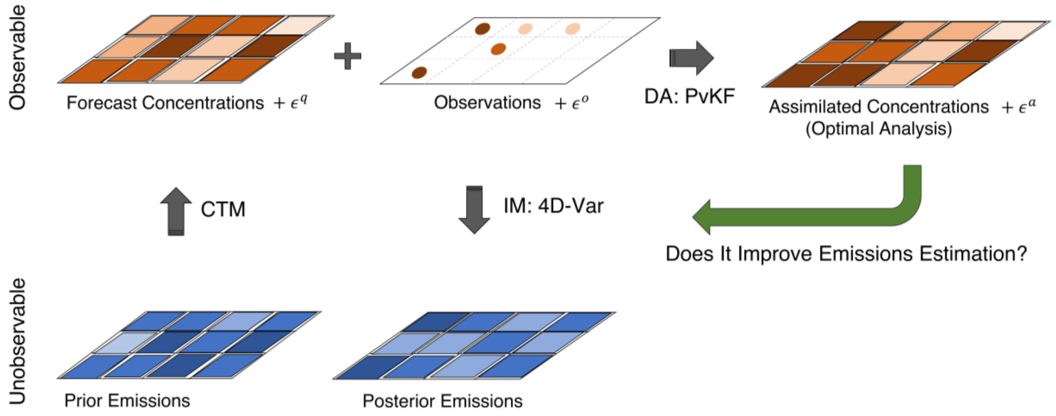
2.3. Overview of the Assimilation and Inversion Systems

2.3.1. PvKF Assimilation

The assimilation scheme performed here is a simplified form of the Kalman filter (not of an ensemble Kalman Filter) for estimating methane concentrations. This algorithm is based on a parametric variance Kalman filter (PvKF), where the correlations are assumed to be homogeneous and isotropic, and the dynamics of the error variance are approximated using only advection. The idea of evolving only error variance with an advection scheme emerged in Kalman filtering by Cohn, 1993 [60], and the first practical atmospheric implementation was demonstrated by Menard et al., 2000 [61]. The design and implementation of the PvKF assimilation with the CMAQ model have been detailed in Voshtani et al., 2022a,b [34,38]. One main objective of developing the scheme was to reduce the computational cost of state assimilation while avoiding the challenges in the previous approaches, such as EnKF and 4D-Var. In fact, the assimilation requires only two model integrations, one for the state and the other for the error variance. Despite its simplicity, it was shown that the method is well-adapted for the assimilation of long-lived species, such as methane, without loss of variance.
The assimilation system maintains an error covariance function ( P ) of the form
P   =   σ   C   σ ,
between each pair of model grid points, where σ and   σ   are the standard deviations of forecast error at two different grid points and time t , and C denotes the correlation function based on the second-order autoregressive (SOAR) correlation model. According to Voshtani et al., 2022a [34] C has the form
C = C S O A R   =   1   +   D L exp D L ,
where D is a chordal distance between the position vector of a pair of grid points on the surface of the sphere, and L denotes the correlation length scales. Based on the cross-validation method [62], the estimated horizontal and vertical length scales, as used in this study, are chosen: L h = 350 km and L v = 7 σ l ( σ l denotes the model vertical layer, starting from the surface, based on the sigma-pressure coordinate system). Note that the error correlation function is never stored as a matrix but is computed during the simulation, as we need the correlation between a pair of points, and thus there is no requirement to store a large matrix in the model state space. Future details of the algorithm and assumptions associated with the input error covariances are described in Voshtani et al., 2022a,b [34,38].

2.3.2. 4D-Var Inversion

The inversion procedure is based on a typical 4D-Var algorithm, relying on the CMAQ model and its adjoint [63,64] to optimize methane emissions in the Northern Hemisphere. The adjoint of CMAQ has been validated and used previously in different inversion studies [65,66]. We integrate the adjoint model based on the same version and chemical mechanism used in the CMAQ model. To optimize surface methane emissions in a formal 4D-Var inversion, we seek to minimize the cost function in the form of
J ( x ) = 1 2 γ ( x x b ) T B 1 ( x x b ) + t = 0 n 1 2 y t o H t ( c i , x ) T R t 1 y t o H t ( c i , x ) .
where x = log e / e b denotes the log-transformed emission-scaling factors, x b represents the corresponding scaling factor of the baseline emissions ( e b ), n is the number of the hourly timesteps, y t o is the methane observations for the timestep t, c i denotes the initial model concentration field, and H t represents the observation operator that applies on c i and x while, at the same time, it maps the model state into the observations space. B and R denote error covariance matrices of prior emissions and observations, respectively, and γ is a regularization parameter. We will briefly explain these parameters later in this section.
Accounting for Equation (3), we correct for monthly mean methane emissions ( e ) at 108 × 108 km resolution using variational optimization, which is an iterative procedure [25,30,31,67,68]. In fact, the gradients of the cost function with respect to the methane emissions are computed at each hour using the CMAQ adjoint model. Those gradients are used to obtain emission-weighted monthly mean sensitivities of emission-scaling factors in each grid cell. At the end of the iteration, the sensitivities are supplied to a quasi-Newton limited-memory optimization routine, L-BFGS [69], for which we use the “optimr” package in R. Using the new scaling factors provided by L-BFGS, updated emissions are obtained and used in the next iteration. We assume that the convergence of this procedure occurs once the reduction of the cost function in consecutive iterations remains less than 1%.
A conventional method in inverse modelling to balance the weight of the prior constraint in the cost function is to use a global regularization parameter γ [66,67,70]. It is also interpreted as an approximated compensation for the missing objective information in quantifying error correlations in R [22]. The estimation of the regularization parameter is performed by inspection and by conducting a series of 4D-Var inversions while choosing the parameter γ that minimizes the cost function J (Equation (3)) among all optimal experimented estimations. Accordingly, we found the value of γ = 900 as our best estimate (see Figure S1 for details). The observation error covariance is considered diagonal with a form of R = ( ε o ) 2 I , where the observation errors ( ε o ) are proportional to the measurement errors ( ε o = f o ε m ), and the estimated factor, f o , is obtained using the cross-validation technique [38]. For matrix B, we have adopted a simple approach that the emission errors are assumed to be uncorrelated in space and between sectors, making B a diagonal matrix. In fact, we give the same error weight geographically and for all sectors, resulting in an emissions-weighted matrix with 100% uncertainty in each grid cell.

2.4. Using PvKF Assimilation Analysis in 4D-Var Inversion: The Formulation

A common assumption typically made in 4D-Var source inversion is that the uncertainty in the initial state is negligible compared to the accumulated effect of emissions uncertainty over a long period of time. With such an assumption, there is no dependency on the initial state uncertainty in the 4D-Var cost function (Equation (3)). This is equivalent to considering the initial concentrations close to the true estimate [12,32,33,45,46,71].
Here, this paper employs a different approach for estimating methane emissions using the 4D-Var algorithm. In fact, we make the initial state uncertainty as small as possible by assimilating observations prior to the 4D-Var inversion window. Furthermore, using PvKF assimilation, we will know what is the analysis uncertainty at the beginning of the 4D-Var window. Figure 2 shows the assimilation window (the blue bar or T 0 1 = T 0 , T 1 ) alongside the inversion window (the yellow bar or T 1 2 = T 1 , T 2 ) and how they interact with each other. The PvKF assimilation starts with the initial condition derived from the global modelling and measurement data [52] and computes the error variance at the end of the assimilation time window, T 1 . As part of the assimilation, an estimation of the modelling error covariance ( Q ), observation error covariance (R), and background correlation length ( L c ) are obtained using the method of cross-validation and innovation variance consistency demonstrated in Voshtani et al. (2022b) [38]. These estimated error statistics will be an informative supply to the subsequent experiments performed in this study. At the end of the PvKF assimilation window, the analysis field ( c 1 a ) and the analysis error covariance ( A 1 ) are obtained and will be used for the purpose of inversion (Figure 1). Note that 4D-Var here integrates the same type of observations (i.e., column retrievals of GOSAT methane) as used in PvKF assimilation but for a different period of time to avoid double-counting.
As shown in the rest of Figure 1, four main types of experiments are designed to investigate the role of state concentrations and their uncertainties for emissions inversion. The difference between these experiments depends only on the assumptions used to initialize the field and propagate the error uncertainties during the inversion window. Although the details of performing these experiments are presented in the next section of OSSEs, here we briefly describe their main differences. In experiments 1 and 2, the model forecast and the PvKF assimilation generate the concentration field, c 1 f and c 1 a , respectively. These fields are assumed to be perfect; thus, there is no associated uncertainty to be propagated during the inversion window. On the other hand, experiment 3 not only accounts for the initial state uncertainty ( A 1 ) but includes the effect of propagating it during the inversion. To propagate the errors, we use the PvKF algorithm capabilities that adapt an advection scheme. In experiment 4, we expand on experiment 3 by including modelling error (i.e., Q ), which is separately estimated for the inversion window. Note that the modelling error Q must be distinguishable from (model) transport error or forecast error P f (i.e., model-propagated initial error); accordingly, model error Q is assumed to be zero in experiments 1–3 due to a perfect-model assumption.
In the context of an OSSE (Section 2.5), we need to generate the observations from the true state. Since the PvKF optimal analysis can be considered as the closest estimate of the true state, we thus have
y 1 2 f = H ( c 1 a , x t ) + ε 1 2 f
y 1 2 o = y 1 2 f + ε o
where y 1 2 f is the model forecast mapped on observations time and location using the observation operator H o . In Equation (4), H includes both model ( M ) and the observation operator ( H o ), such that H ( c 1 a , x ) = H o M ( c 1 a , x ) . ε 1 2 f represents the model transported analysis error up to the current forecast time, and ε o is the observation error used to construct R. The associated forecast error covariance for the inversion window is denoted as P 1 2 f = P f ( A 1 , Q ) . It is obtained by
P t f = Σ t f C   Σ t f
where Σ t f is the diagonal matrix of forecast error standard deviation ( σ t f ), where the corresponding forecast error variance is computed using the advection-only scheme (see Section 2.3.1). C is the matrix of error correlations which is derived from Equation (2).
Now, let us define a new form of the cost function for performing our inversion. In this case, other than the observation errors that affect the innovation (i.e., Observations–Model; see Equation (3)), we have to account for the propagated analysis error in the inversion window. The analysis error at time T 1 depends on the observations in the window T 0 1 . Since the observation errors are assumed to be temporally uncorrelated, the analysis error, ε 1 a , is uncorrelated with the future observations used in the inversion window ( T 1 2 ). Hence, the innovation ( y t o H t ( c 1 a , x ) ) initialized by the analysis field should have an error weight of the form H o P t f ( A 1 , Q ) H o   T + R (i.e., innovation error covariance) in the cost function. This is a sum of the two terms, indicating that their contributions are uncorrelated. Since this typically large-size matrix may no longer be diagonal, inverting it is a challenging process. In Appendix A (Figure A1), we present a practical approximation using a data selection approach to deal with the matrix inversion of such matrices. Finally, the modified form of the cost function that is appropriate for our two-part scheme is presented in Equation (7) of Table 2. Other variants of the cost functions used in our OSSE experiments are illustrated in Section 2.5.2.
Table 2. Cost functions for different formulations of 4D-Var inversion. P t f is the model-propagated (forecast) of error covariance in the model space, A 1 is the analysis error covariance at the initial time of inversion, and Q is the modelling error covariance that is estimated independently (see Section 3.1). c 1 f and c 1 a represent the initial field of concentrations produced from the hemispheric CMAQ model and PvKF assimilation, respectively. * Type 0 is the form of the 4D-Var cost function proposed by this work.
TypeCost Function
Type 0 *: J 0 ( x ) = 1 2 γ ( x x b ) T B 1 ( x x b ) + t = 0 n 1 2 y t o H t ( c 1 a , x ) T H o P t f ( A 1 , Q ) H o   T + R t 1 y t o H t ( c 1 a , x ) (7)
Type 1: J 1 ( x ) = 1 2 γ ( x x b ) T B 1 ( x x b ) + t = 0 n 1 2 y t o H t ( c 1 f , x ) T R t 1 y t o H t ( c 1 f , x ) (8)
Type 2: J 2 ( x ) = 1 2 γ ( x x b ) T B 1 ( x x b ) + t = 0 n 1 2 y t o H t ( c 1 a , x ) T R t 1 y t o H t ( c 1 a , x ) (9)
Type 3: J 3 ( x ) = 1 2 γ ( x x b ) T B 1 ( x x b ) + t = 0 n 1 2 y t o H t ( c 1 a , x ) T H o P t f ( A 1 ) H o   T + R t 1 y t o H t ( c 1 a , x ) (10)

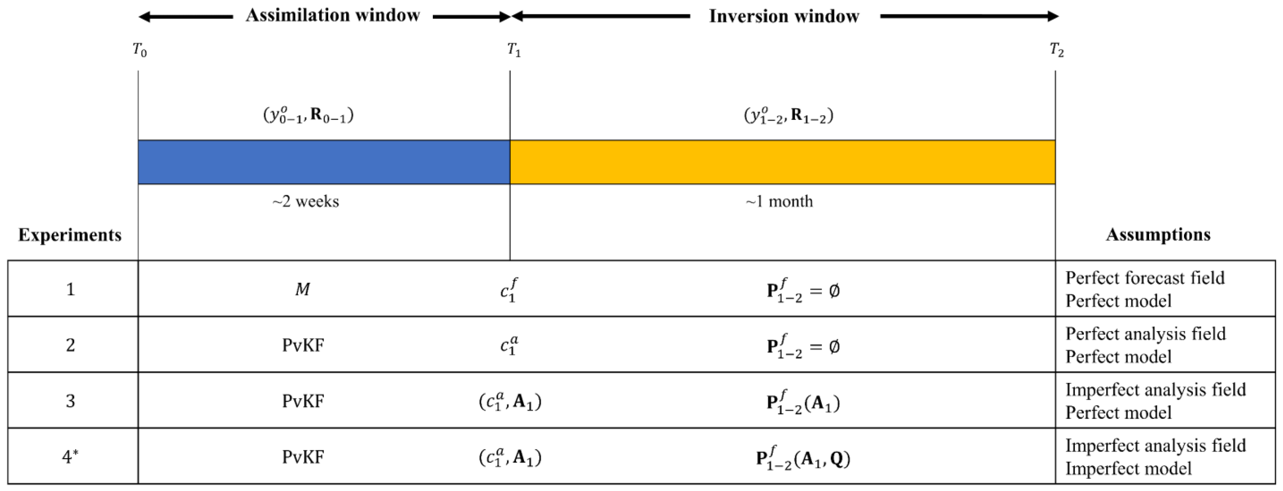
2.5. Description of the OSSE Experiments

OSSE is a standard method to evaluate the performance of atmospheric inversion or assimilation systems without using the actual observation data [72]. Our OSSE experiments are designed with simulated GOSAT observations to verify how optimal state analysis and its propagated uncertainty may improve a 4D-Var inversion for constraining methane emissions. Accordingly, we test different effects of the model state on the source inversion (see Section 2.4, Figure 2). To distinguish those effects, we evaluate the OSSE using different forms of 4D-Var cost functions across several emissions perturbation types, and we discuss various aspects of those effects. The basic description of the OSSE setup and emissions perturbations are provided in Section 2.5.1, followed by explanations of the cost function variations in Section 2.5.2.

2.5.1. Perturbation Tests

Figure 3 shows the generic design of an OSSE framework. The structure of every OSSE system consists of two main parts: A nature run and control runs [7]. Through a nature run, the CMAQ model forecast produces the synthetic (true) concentration field to be sampled by the observation operator, providing simulated observations. The nature run is derived by the initial analysis field of concentrations at time T1, meteorological field from WRF output, and anthropogenic and natural methane emissions that are taken the same as provided by corresponding inventories (see Section 2.2). It is assumed that both inputs and the model CMAQ in the nature run are deterministic, comparable to a mean estimate of a stochastic process. On the other hand, the simulated observations are not assumed to be perfect but include GOSAT observation errors. Hence, the simulated observations are imperfect only due to observation errors.
The observations generated through a nature run are used under a controlled environment to perform different inversion and assimilation runs. Those are conducted within control runs (also known as perturbed runs), for which different forms of initialization, error statistics, and emissions perturbations are configured for the inversion window (Figure 3). Therefore, control runs only cover the inversion window but include the effects of the assimilation window by providing the initial field and/or initial error covariances at time T 1 .
Besides the four types of cost functions that will be described in Section 2.5.2, we consider three forms of perturbations to produce different distributions of the prior methane emissions in the control runs. Those perturbations reflect uniform and variable biases in the prior methane emissions and cover both total and sectoral emissions. Note that in all our control runs, we assume imperfections in the state concentrations and the CTM, but we apply the same meteorological field, chemical reactions, and boundary conditions as used in the nature run. Thus, these processes are considered perfect, and their effects (i.e., potential errors or biases) are not investigated for the objective of our OSSE experiments in this study.
Using the OSSE framework (Figure 3), we can compare posterior and the prior emissions against true emissions. Accordingly, the main goal of our OSSE experiments is to test the ability of our proposed inversion cost function (Equation (7)) to reproduce true methane emissions. In addition, by exploring three other variations in the cost function (see Section 2.5.2), we aim to address the limitation of a typical 4D-Var inversion that relies on perfect state assumptions due to the initial field or the CTM (meteorology and chemistry are excluded). The approximation of diagonal observation error covariance is also evaluated in our OSSE experiments.

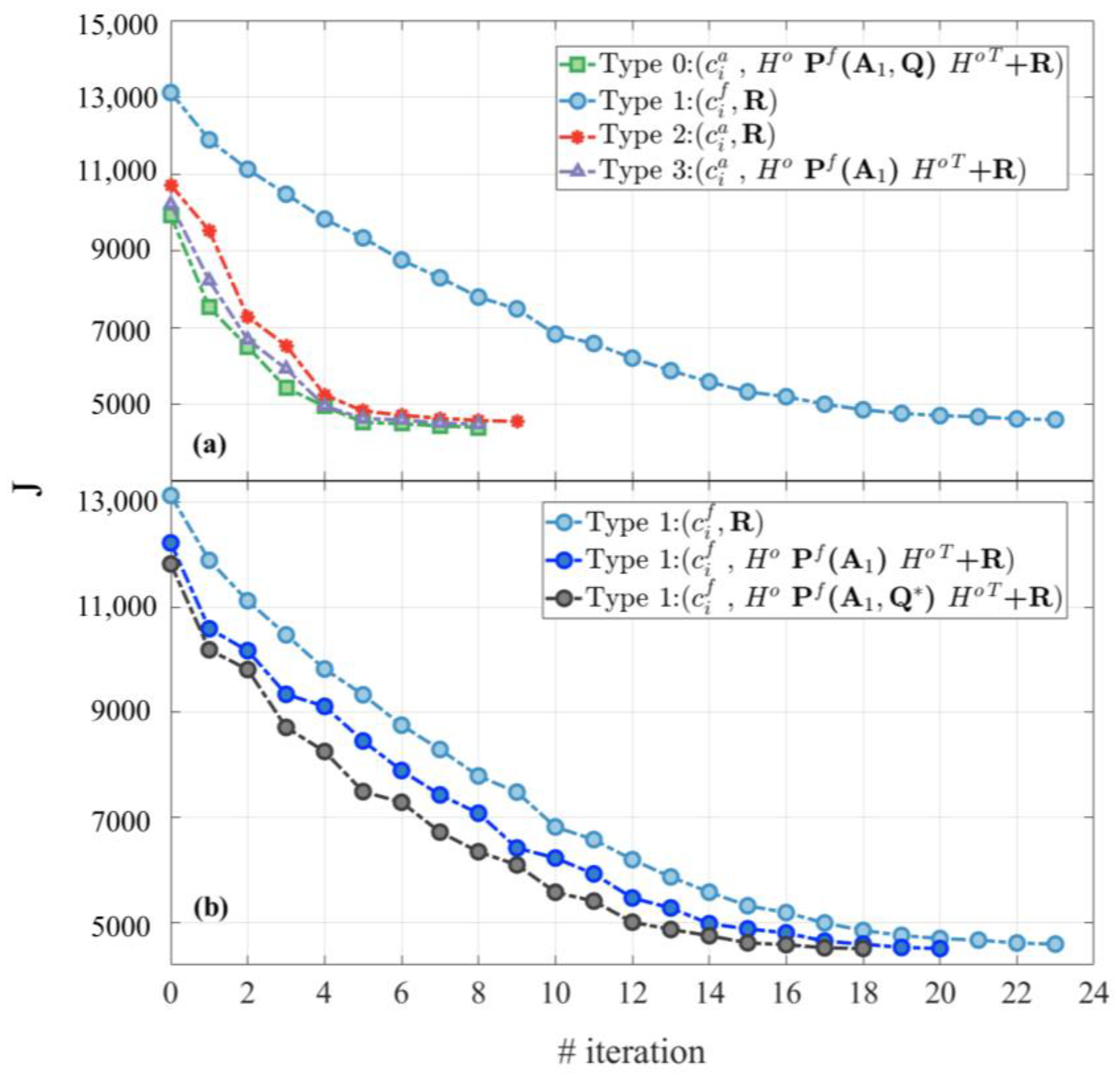
2.5.2. Experimenting with Different Cost Functions

Table 2 summarizes four variations of the 4D-Var cost function. We recall that for this study, the inversion does not necessarily rely on a perfectly known initial state or a perfect forward model assumption. We start with Type 0 (Equation (7)) as the principal form of the cost function proposed in this study. In this equation, we account for the entire information provided by PvKF assimilation, including the initial analysis field ( c 1 a ) and its analysis error covariance ( A 1 ). In addition, according to the PvKF formulation for propagating errors using the advection scheme (see Section 2.3.1), the forecast of the analysis error covariance and the estimated model transport error ( P t f ( A 1 , Q ) ) are integrated into the second term of the cost function. Inversions of Type 1–3 (Equations (8)–(10)) consider other forms of cost functions where parts of the connection between the assimilation and inversion are broken. For Type 1 (Equation (8)), we neither consider the analysis field nor the propagation of the error covariances (i.e., P t f ( A 1 , Q ) = 0) during the inversion. In fact, inversion is independent of assimilation and is initialized by the model forecast, which is assumed to be perfectly known. In this case, the inversion also only relies on the observation error covariance ( R t ) in the cost function. Note that the cost function of Type 1 is frequently used in different inversion studies [42,46,55]. Type 2 inversion (Equation (9)) is similar to Type 1, except that it begins with the initial analysis field rather than the initial forecast concentrations. Type 2 cost function is also commonly used in the literature [32,33,73]. Type 3 (Equation (10)) not only accounts for the initial analysis field but also considers the propagation of its error covariance during the inversion, yet with a perfect model assumption (i.e., Q = 0). Note that we keep γ , x b , and B the same between all these cost functions for consistency of our evaluations.
By comparing all the cost functions in Table 2, we can distinguish the different effects of using assimilation for performing a 4D-Var inversion. Accordingly, a comparison between Type 1 and Type 2 cost functions shows the influence of only the analysis initial field on the inversion result. By comparing Type 2 and Type 3 cost functions, we can isolate the effect of considering the uncertainties in the model concentrations that originate from the initial state (i.e., model-propagated initial error covariance). Finally, if we compare Type 3 with the Type 0 cost function, the influence of model error covariance Q (separately estimated) on the inversion can be extracted.

3. Role of Assimilation in Improving Inversion Results

Our results of the OSSEs include a month of posterior (i.e., optimized) methane emissions in April 2010 using 4D-Var inversion, preceded by two weeks of PvKF assimilation (or model forecast when the assimilation is turned off). Note that, in this study, we will not explore a temporal trend of emissions, such as seasonal and annual biases, but will mainly focus on optimizing the spatial distribution of emissions in a shorter time scale (e.g., episodical emissions inversion) that are more subjected to different types of biases at the state concentration level. The posterior emissions estimate involves monthly mean methane emissions, or in particular, emission scaling factors. The following sub-sections (Section 3.1, Section 3.2 and Section 3.3) are each dedicated to the results of a specific form of emissions perturbations throughout the OSSEs. These perturbations result in a particular form of the prior emissions in our control runs (see Figure 3). We recall that all the input and configurations are the same for all experiments (e.g., meteorological field, regularization parameter γ ), except those that impose the discrepancy between the OSSE cases (Figure 3).

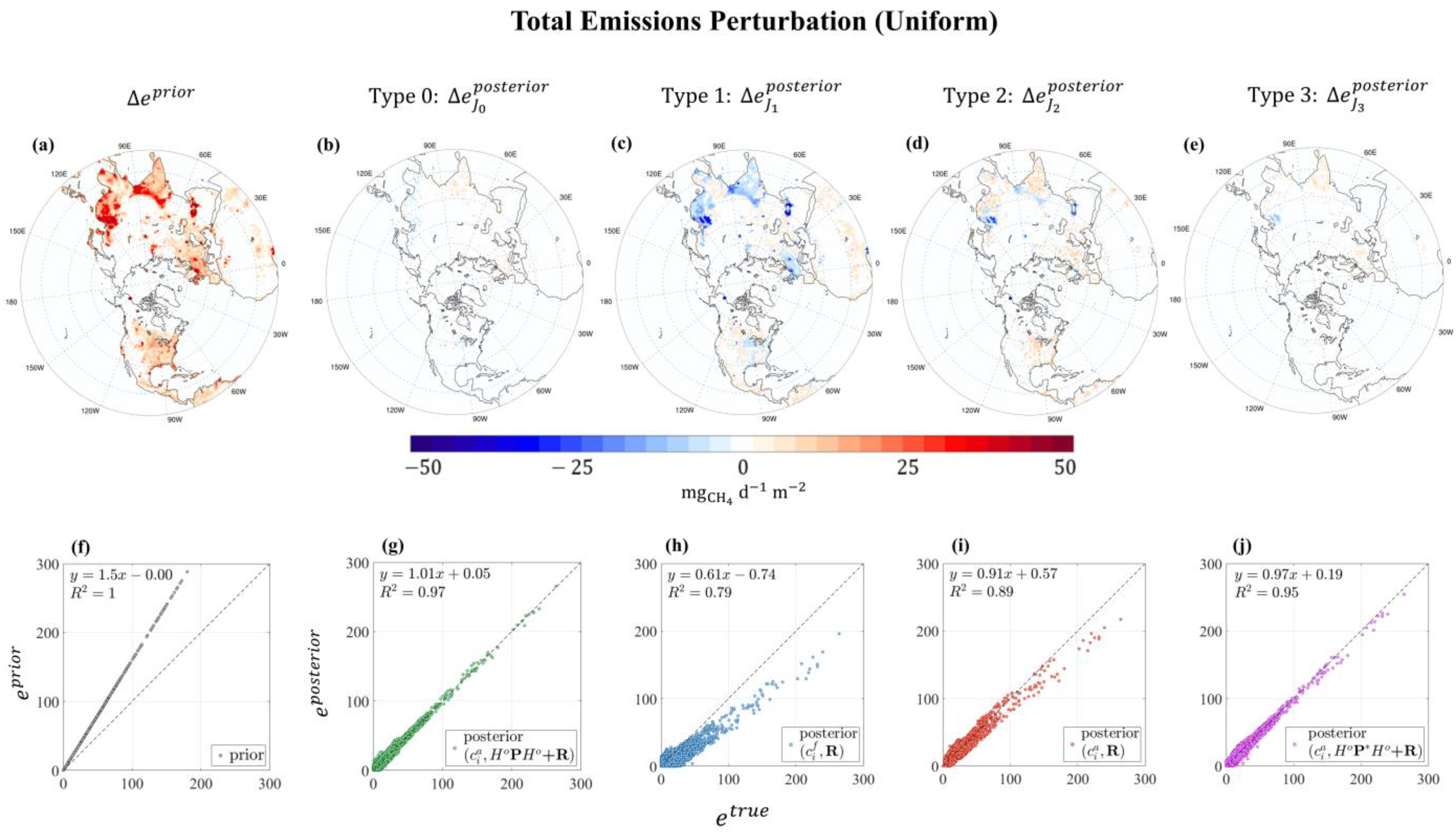
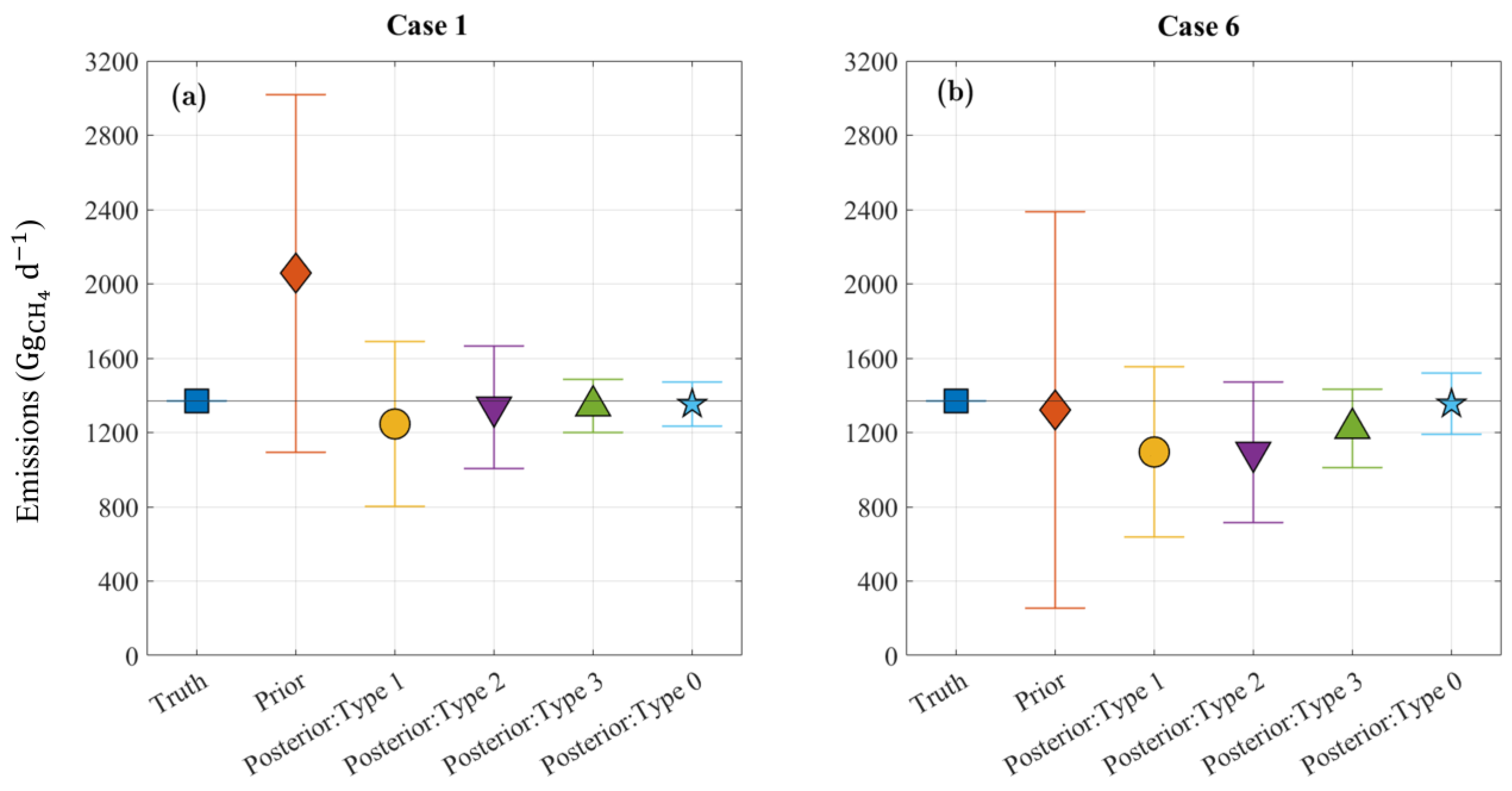
3.1. Perturbation of Total Emissions

The first type of perturbation provides the prior emissions with a uniform bias in all sectors (see OSSE control runs in Figure 3). In this case, the total true emissions are uniformly scaled up by 50%. In fact, it is assumed that the prior emissions are strongly in line with the spatial distributions of the true emissions, yet with different levels of magnitude. Although this perturbation method implicitly considers a low level of uncertainty for the spatial allocation of emissions, it can be taken as the base case, particularly for evaluating the ability of the inversion method and underlying assumptions to reproduce true emissions [29,39,74].
Figure 4 compares the posterior emissions of the four inversions according to the cost functions in Table 2. All inversions start with the same prior with +50% uniform perturbation of the true emissions. The spatial distributions of the differences between the prior and true emissions ( Δ e p r i o r ) and between all four posteriors and true emissions ( Δ e p o s t e r i o r ) are shown in Figure 4a–e, respectively. Type 0 inversion (Figure 4b) accounts for both optimal PvKF analysis ( c 1 a ) and model-propagated (forecast) of analysis error covariance during inversion ( P t f ( A 1 , Q ) ). Posterior emissions show reasonable overall consistency with the true emissions, particularly for the larger and more local (or point) sources. Now, we remove all the dependency on the assimilation such that a perfect model forecast ( c 1 f , P = 0) is linked to the inversion (Type 1). In this case, the corresponding initial condition is far from the truth. The corresponding posterior emissions in Figure 4c indicate a large deviation from the true emissions. In fact, a significant (downward) over-correction in many regions, especially for the large sources, is obtained along with an insufficient correction for the small sources. This behaviour first implies that relying on a model forecast with a perfect assumption to initialize the inversion exerts a substantial impact on the state of the system, mainly due to accumulating incorrect emissions before inversion (i.e., the prior emissions are incorrect). Hence, this eventually degrades the emissions estimation through inversion. Furthermore, the prior error covariance (B) is commonly assumed (uniformly) to be proportional to the emissions in standard 4D-Var inversion (as used in this study). This itself also limits the ability of the inversion to recover fairly large and small (scattered) sources, as also suggested by Yu et al., 2021 [39]. In addition, the inversion performance can be worsened in the presence of an incorrect state and missing modelling error correlations.
In Type 2, the inversion is performed with the PvKF analysis ( c 1 a ), which is used as the closest estimate to the true state. Figure 4d shows that using the PvKF optimal analysis field in the inversion instead of a model forecast largely improves the posterior emissions estimate. This is likely because the analysis increment during the inversion corresponds more significantly to the correction of the prior emissions, not the initial field. Note that all the inversions here optimize only for the emissions; thus, a more accurate (and unbiased) initial field that is produced by the optimal analysis can result in better performance of the inversion to recover true emissions. Still, the analysis uncertainty is not taken into account in Type 2 to propagate errors during the inversion, meaning that the concentration field is perfectly known. Thus, we only rely on the observation error variance (diagonal matrix R) in the corresponding cost function (Equation (9)). For this case, although Figure 4d shows an overall improvement in the posterior emissions estimates compared to Figure 4c, it remains inaccurate, particularly in the regions with large amounts of methane emissions, such as East Asia and around the Persian Gulf, and for emission sectors with larger area coverage such as agriculture in the Midwestern United States and India.
However, comparing the posterior emissions of Type 2 and Type 3, we might infer that, besides the analysis field, accounting for the analysis error covariance and propagating it during the inversion can significantly improve the emissions estimates. This is mainly due to the structures of the correlations that exist in the model forecast (see Appendix A, Figure A1), while it is usually neglected due to perfect model assumptions or for computational purposes [22]. Errors in the forecast during the inversion can be produced by the model due to various effects [18,26] or can be the result of an initial error that is propagated through the model, both of which are important to be considered besides the observation errors for a realistic estimation problem.
In Type 3 inversion, a similar condition as Type 0 is considered, except that the modelling error ( Q ) is turned to zero. This depicts a scenario where the model is assumed to be perfect, but in our experiments (and in reality), it may not necessarily maintain the optimal state (closest to the true). Drawing a comparison between Figure 4e (Type 3) and Figure 4b (Type 0) shows minor global differences, although over some larger emissions regions, such as East Asia, that discrepancy still remains noticeable. This is likely due to the lower density of the GOSAT observations over those regions, for which adding model error ( Q ) makes those observations more impactful for the inversion. Hence, accounting for model errors Q in 4D-Var inversion provides room for improvement, particularly when observations are insufficient. On the other hand, comparing either Type 0 or Type 3 against Type 2 inversion indicates that a considerable improvement occurs for both large and small sources. This emphasizes the key role of the model-propagated error correlations (initialized by the analysis error covariance, H o P t f ( A 1 , Q ) H o   T ) that are usually overlooked in an inversion with perfectly known state assumptions and diagonal observation error covariance.
OSSE experiments aid in determining the statistics of the posterior emissions without a need to estimate those along with the inversion, which otherwise entails a high computational cost [30,43]. Accordingly, besides the spatial maps, the prior and those four optimized emissions are demonstrated in scatter plots, as in Figure 4f–j. Figure 4h indicates that Type 1 inversion, which integrates the biased model initial forecast (due to biased emissions before the inversion), can result in fairly biased posterior emissions along with significant variance. Accounting for the initial analysis field in Type 2 inversion improves on the bias of the optimized emissions while slightly decreasing the variance (Figure 4i). On the other hand, propagating the analysis error (comparison between Figure 4j,h) can largely affect the variance of posterior emissions, although with a small bias improvement.
Overall, adding the model error, Q , (comparison between Figure 4g,j) can further improve the bias (and slightly the variance) in posterior emissions, particularly for the larger sources, as in Figure 4e,b. Additionally, the posterior emissions in Figure 4g maintain an estimate that is also statistically more reliable than other inversion types, although it tends to be less reliable for estimating small sources. This deficiency is likely due to limited information in determining the prior error covariance (B) for properly weighting the prior emissions [22,39].

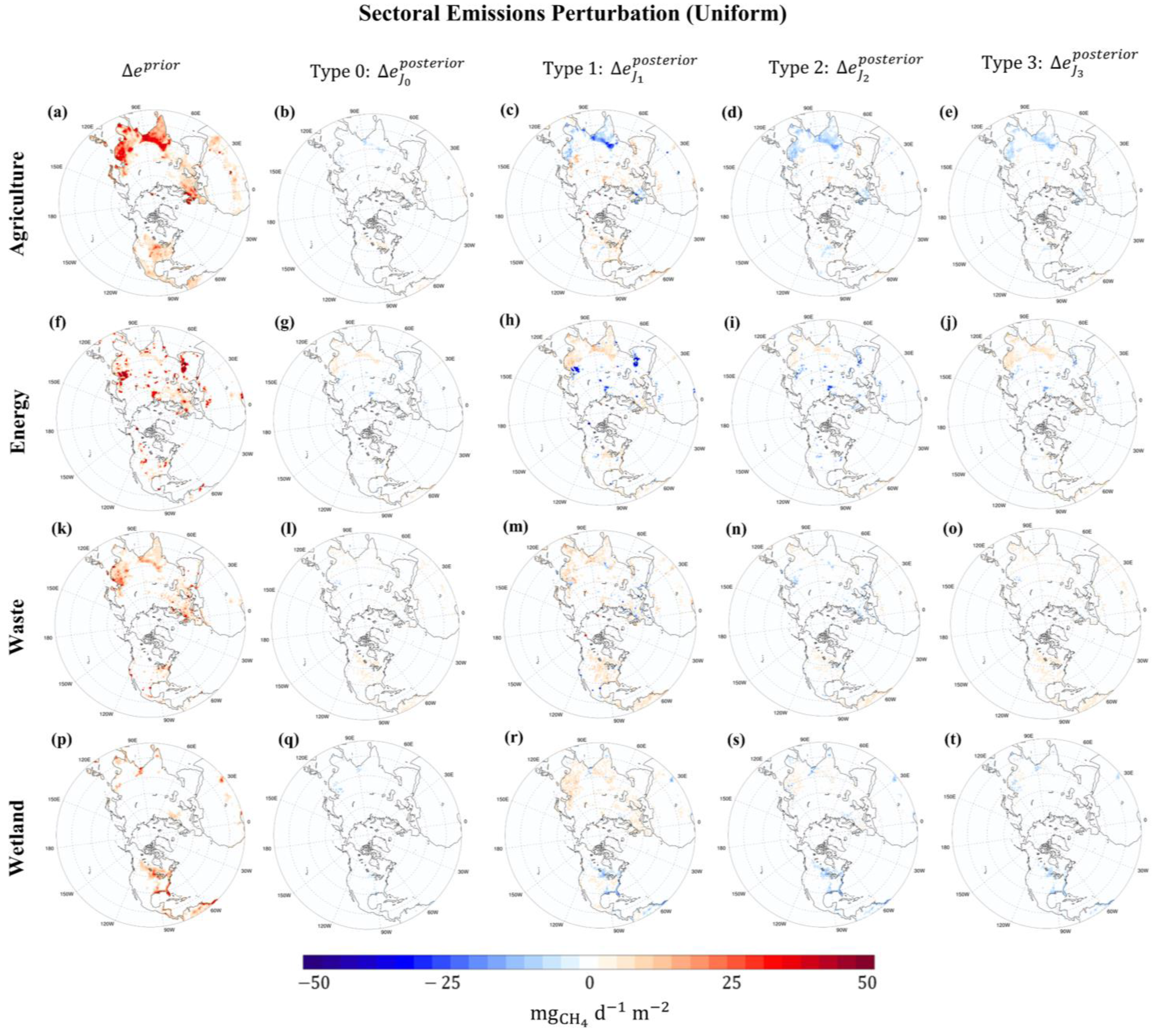
3.2. Perturbation of Each Sector

In the second form of perturbation used in our OSSE experiments (see Figure 3), we examine the ability of our inversion to reproduce true emissions when only one particular emission source sector is perturbed. Following the four main emissions categories in Table 1, each source sector is uniformly perturbed in the same way as the total emissions perturbed in Section 3.1 (i.e., scaled up by 50%). We repeat inversions with different cost functions (i.e., Equations (7)–(10)) for this experiment. Figure 5 presents the spatial distributions of the differences between the total prior/posterior methane emissions and the true emissions, in which every map corresponds to a specific sectoral perturbation that is performed with a particular inversion type.
The overall spatial pattern of the posterior emissions in each sector shows the same order of improvement as obtained for the total emissions in Section 3.1. In fact, the contribution of the PvKF analysis field, used as the initial condition, and its error covariance to the inversion leads to a better constraint for every sector. However, the responses of each source sector to different types of inversions are not the same. Before discussing the inversion response (see details in Section 4.1) in each sector, we need to reacquaint ourselves with some characteristics of each sector, which can be addressed from the figures with prior perturbations (Figure 5a,f,k,p). Besides the geographical locations of the prior emissions in each sector, it is important to identify their spatial distribution along with the density of each sector’s prior emissions. According to those criteria, we consider agriculture and wetland emissions as area sources (covering large areas with an almost uniform level of emissions), while the emissions of the energy sector are considered as local or point sources (covering small or local areas with large amounts of emissions; hotspots). Although waste emissions appear in both area and point sources depending on their location, overall, across the domain, we consider it in the point-source category (Figure 5k). All these specific characteristics enable us to evaluate and distinguish the differences between the responses of each sector to the inversion. Note that the magnitude of those emission sectors is largest for wetlands, followed by agriculture, energy, and waste.
For Type 1 inversion, the posterior emissions for each sector show an overestimation of large emissions and an underestimation of smaller emissions in the same sector. We also found that the biased forecast initial state may cause a miscorrection on other emission sectors, even though they are not perturbed (i.e., taken as true emissions) in the prior emissions—hereafter, this is considered as the effect between sectors and referred to as the cross-sectoral effect. For example, the posterior of the agriculture emissions in Figure 5c shows an apparent overestimation of emissions at the locations of the energy sector’s emissions (e.g., over Russia and near the Persian Gulf). However, this impact is largely removed for the Type 0 inversion of the agriculture emissions (Figure 5b), which is consistent across all sectors’ perturbations. This implies that a configuration of inversion that integrates the optimal initial analysis and its error covariance propagation not only performs reasonably for the incorrect emissions of the same (perturbed) sector but can also prevent misrepresentation of other sector’s emissions when they are precisely provided in the prior.
Comparing the results of Type 1 with Type 2 inversions reveals the effect of initializing the inversion with the assimilation analysis field rather than the model forecast field. Figure 5c,d (same as Figure 5h,i, Figure 5m,n, and Figure 5r,s) shows meaningful improvements in the posterior emissions from Type 1 to Type 2 for all sectors; however, those improvements are slightly greater for the energy and waste sectors with localized emissions than agriculture and wetlands. A similar improvement (in the same perturbed sector) has been found when we compare Type 2 with Type 3 inversions, for which the forecast of the analysis error covariances is considered besides the analysis field (Figure 5d,e). Although those improvements are more substantial for the energy and the waste sector, a slight degradation occurs in other unperturbed sectors due to a cross-sectoral effect. For instance, comparing Figure 5i,j of the energy sector indicates that despite the improvement of the emissions in the location of the energy sources (e.g., East Asia and Russia), it causes a cross-sectoral effect on the agriculture emissions, resulting in degraded estimate over those areas (e.g., India and Southeastern Asia). A similar pattern is also shown in the waste sector (Figure 5n,o), where the estimation over agriculture and wetland areas is slightly worsened (e.g., Midwestern U.S. and Boreal regions in North America). Nevertheless, we found that the cross-sectoral effect is not noticeably destructive to the inversion of agriculture and wetland emissions (Figure 5d,e,s,t) when we account for the analysis error covariances in a Type 0 inversion (Equation (7)). All that considered, the undesirable cross-sectoral effect suggests that the approximated correlation model (Equation (2)) with a fixed correlation length across the domain is not sufficiently informative to resolve the structure of the large and localized emissions in the energy and waste sectors. Furthermore, we imply that the weight of the forecast error covariance ( H o P t f ( A 1 ) H o   T ), compared to the observation error (R), is likely too small for those sectors; thus, the estimation system relies more on the model and the prior information (which are more uncertain) than on the observations to correct emissions. One way to partly alleviate this is to increase the forecast error covariance by adding extra (bulk) model error ( Q ). We consider the effect of this model transport error in the remainder of this section.
Comparing Type 3 with Type 0 inversion helps us understand the influence of model error, Q , in reproducing true emissions. From an estimation point of view, model error compensates for those missing error variances and correlations that are, in fact, unexplainable by the error propagation scheme (i.e., advection of variance herein; see Section 4.2 for details). Our results show that accounting for the model error ( Q ) improves emissions estimation for all sectors (Figure 5b,e; Figure 5g,j; Figure 5i,o; Figure 5q,t). However, this level of improvement is larger for the agriculture and wetland than for the energy and waste sectors. For example, adding the estimated model error to the Type 3 inversion of agriculture emissions (Figure 5b,e) can substantially remove the underestimate in the posterior emissions, particularly over Northern India and Southeast Asia. A similar level of improvement for the wetland emissions over the boreal region and the Southeastern United States is observed (Figure 5q,t). The influence of model error, however, is not as significant for the point sources of energy and waste emissions. Nevertheless, adding model error can still be important for the cross-sectoral effects of a sector primarily composed of point sources (e.g., energy) on a more spatially distributed sector. For instance, for the inversion of energy (Figure 5j) and waste (Figure 5o) emissions, the overestimation of the agriculture (e.g., Southeast Asia) and wetland (e.g., boreal area) emissions are slightly removed by adding model error Q (comparing with Figure 5g,l).
In our estimation, the model error ( Q ) is assumed to be proportional to the variance field, in line with the previous study by Voshtani et al., 2022a [34]. It provides a uniform and bulk impact on the total error across the domain (see Section 4.2) due to a rather homogeneous distribution of methane. Therefore, as expected, those emission sectors covering the broader area, such as agriculture and wetland, are more susceptible to being influenced by the model error. On the other hand, the model error has less spatial variability than the emissions and thus has little chance of affecting a point-source estimation, even though it may have a large magnitude. Perhaps another form of model error, for which the spatial pattern is different, may improve the influence of model error on the local and large sources, such as energy and waste emissions. The simple fact that the correction for the point sources is not as efficient may indicate that the estimation of the point sources and area sources should be treated with a different modelling framework. In general, due to limited information and large uncertainty about the origin of model error, finely resolving its spatial structure is typically a nontrivial task [25,75]. Note that we do not separately obtain an estimation of model error for each inversion process of this study; instead, we apply the estimated parameter following Voshtani et al., 2022b [38] (see Section 3.1 for details). Thus, the error variance associated with the model may also not be the optimal one in our analyses here. A statistical comparison of the prior and the posterior emissions against the true emissions is also demonstrated in Figure S2 in Supplementary Materials.

3.3. More Realistic Perturbations

OSSE experiments in this section consider a more realistic inversion scenario, aiming to provide a random-like (more objective) perturbation in the prior emissions. One way to achieve this is to perturb each sector individually with different weights and signs ( ± ) of perturbations while taking them all together for the inversion analysis. Previous methane inversion studies [2,12,21,76,77] showed that, overall, agriculture and waste emissions are underestimated, whereas the energy and wetlands are overestimated globally in the prior (mainly based on EDGAR for the anthropogenic inventory and WetCHARTs for the wetlands). Thus, the energy and wetland sectors are perturbed upwards by 50% and 25%, respectively, and the waste and agriculture sectors are perturbed downwards by 50% and 25%, respectively.
Figure 6 summarizes the performance of our four different types of inversion using these prior emissions. In the Type 1 inversion, the posterior emissions exhibit significant over- and underestimations (Figure 6c). This plot also shows that the weight of the spatial biases in the posterior is almost proportional to the prior emissions, yet agriculture and waste retain a positive bias contrary to the energy and wetlands with a negative bias. Overall, it implies that simply relying on a perfect model initial field results in overcorrections of posterior emissions in many regions. The statistics of the posterior emissions in Figure 6h also indicate that, besides a large domain-wide variance, they are negatively biased in large emissions areas over East Asia (from coal emissions) and near the Persian Gulf (likely due to oil and gas emissions). Furthermore, a lower R 2 and weaker regression line of the posterior than the prior suggests that the posterior emissions are likely less reliable than the prior.
When we compare Type 1 inversion with Type 2, where the PvKF analysis provides the initial state but the inversion relies only on observation error covariance R, we find a significant improvement in the spatial biases of posterior emissions. This is particularly true for the large sources, suggesting that the large domain-wide variance and bias of emissions have been corrected. The R 2 of Type 2 inversion also exhibits a large increase compared to Type 1 but is still comparable to the prior statistics. The Type 3 inversion (Figure 6e,j), which includes the model-propagation of analysis error covariance, maintains a large consistent improvement everywhere compared to the Type 2 inversion. This improvement is reflected in R 2 and the slope of the regression line. The improvement caused by the propagation of the analysis error covariance can be inferred in two ways. First, we know that the state of the system, in reality, is not perfect; thus, the total error is greater than the observation error, R. In this case, relying on a perfect state assumption implicitly gives extra weight to the observations, resulting in under/overestimation of emissions through the 4D-Var inversion. Second, in addition to the weight of the error variance, accounting for the error correlations in P f ( A 1 , Q ) helps the inversion maintain a more realistic distribution of spatial and temporal analysis increments.
The effect of adding model error ( Q ) is also examined. It shows a further improvement of posterior emissions in Type 0 (Figure 6b) relative to Type 3, which is also confirmed by their statistics (Figure 6g). It indicates that adding model error ( Q ) to the forecast error ( H o P t f ( A 1 ) H o   T ) can, in fact, help better constrain the emissions throughout the inversion. In addition to this experiment, we conduct another non-uniform perturbation of those sectors but using different sectoral weights, such that agriculture and wetland are perturbed 50% upwards while waste and energy are perturbed 25% downward (see Figure S3 in the supplements). Overall, we found a similar correction behaviour as the experiment in Figure 6.
In addition, comparing the inversion types of Case 6 (Figure 6) and Case 1 (Figure 4) indicates that both Type 1 and Type 2 in Case 6 provide posterior emissions of higher quality than their equivalent in Case 1, as R 2 increased from 0.79 to 0.82 for Type 1 and from 0.89 to 0.92 for Type 2. The higher quality of emissions of Case 6 can be explained by the perturbation of the prior emissions in OSSEs. In Case 1, entire emissions of all sectors are purebred uniformly upward by 50% (50% increased), but the perturbation of prior emissions in Case 6 is non-uniform (energy and waste emissions are increased by 50%; agriculture and wetlands are decreased by 25%). A simple comparison of these two perturbation cases shows that the overall bias in Case 1 is greater than in Case 6. This bias exists in the prior emissions and may also reflect in the initial field. Given that the inversion only corrects for the prior emissions (not the initial field), we can expect that the inversion of Case 6 provides better posterior emissions than Case 1, likely because the control runs of Case 6 have a lower bias in the initial field and the prior emissions than Case 1. On the other hand, the performance of the posterior emissions of Type 3 and Type 0 in Cases 1 and 6 are more comparable. Perhaps, this is because there is almost no additional source of bias (or uncertainties) than in the prior emissions, not to be captured by the inversion. In fact, the inversion shows a consistent level of performance in different perturbation scenarios once it is not contaminated by the other source of errors (e.g., from the initial condition and its propagation).

4. Additional Discussions for the Proposed System

4.1. Statistical Implications

Three forms of perturbations in our OSSE experiments are described in Section 3.1, Section 3.2 and Section 3.3. We examined the ability of four different cost functions for each perturbation type to reproduce true emissions across the domain. Here, we further evaluate those experiments in terms of three metrics, including normalized mean bias (NMB), normalized mean error (NME), and Pearson’s correlation coefficient. Accordingly, we have
NMB = k = 1 N ( e k e k t ) k = 1 N ( e k t )
NME = k = 1 N e k e k t k = 1 N ( e k t )
R = k = 1 N ( e k t e ¯ k t ) ( e k e ¯ k ) k = 1 N ( e k t e ¯ k t ) 2 k = 1 N ( e k e ¯ k ) 2
where e and e t denote the posterior and true emissions, respectively, and N represents the number of grid cells with emissions.
The results in Table 3 indicate that NMB significantly decreased between Type 1 and Type 2 inversion in almost all emissions perturbation cases, particularly in Case 1 with 28% reduction and Case 6 with 15% reduction, where all sectors are perturbed. It suggests that initialization of the inversion with a biased model forecast ( c 1 f ) reflects on the posterior emissions mainly as a form of residual biases. In addition, NME decreased and R increased for all cases, indicating that the posterior emissions residuals are smaller for Type 2 inversions. In fact, at the grid level, they are closer to the true emissions. Overall, a similar reduction of NMB and NME and an increase of R occurs between Type 2 and Type 3 inversions for all cases. This implies that incorporating the model-propagated analysis error covariance ( H o P t f ( A 1 ) H o   T ) can also substantially impact our inversion results to recover the true emissions. Finally, the effect of the model error ( Q ) is shown by comparing Type 3 and Type 0 inversion. Although we implemented a simple form of Q , the results of all metrics slightly improved for perturbations with all emissions (Case 1, 6, and 7); however, it may influence each sector differently. We found that agriculture and wetland are more sensitive to model error as all the metrics are altered to provide a better fit to the true emission. On the other hand, it has little impact on the energy and waste sector. Those behaviours are mainly attributed to the spatial characteristics of model error that are more consistent with those sectors with broader areas and uniform emissions, such as area sources sectors, including agriculture and wetlands. We provide a detailed discussion of the underlying assumptions for model error ( Q ) as well as its effect on the inversion in the next section.
Aiming to examine the findings of our results in Section 3, we present the total amount of emissions obtained by each inversion type and compare them against the total prior and true emissions. Figure 7 shows the OSSE results of Case 1 with uniform perturbation and Case 6 with non-uniform perturbation of the prior. Each marker denotes the total emissions corresponding to the label on the x-axis. The error bars are computed based on the standard deviation of the difference between the prior/posterior and truth, which is multiplied by the number of emission grid cells to represent an indication of the uncertainty for the total emissions. In Case 1, the posterior emissions of all types are close to the truth (1370 Gg/d), in particular for Type 2, 3, and 0, which are estimated as 1336 Gg/d, 1344, and 1353 Gg/d, respectively. This indicates that using additional information from assimilation analysis may not necessarily improve on the total emissions estimates. However, the map of spatial distributions of those cases (Figure 4) emphasizes a large improvement in different areas for the same types of inversion. It implies that an estimate of only the total emissions can be misleading, since the overestimation and underestimation of posterior emissions in different local areas may cancel out each other and result in an estimation that remains close to the truth. Nevertheless, the estimate of the uncertainties for this case Is still consistent with the previous result, suggesting that the assimilation analysis and propagation of its error statistics result in posterior emissions with lower uncertainties ( σ Type   1 = 444 Gg/d, σ Type   2 = 329, σ Type   3 = 143 Gg/d, σ Type   0 = 117 Gg/d).
Performing a similar assessment on Case 6 with a more realistic perturbation of the prior emissions shows that the total emissions of Type 1 and Type 2 inversions become even worse than the prior emissions. This is also in contrast to the maps of posterior emissions (Figure 6), which show an improvement in the posterior emissions. Comparing Type 0–3 of posterior emissions for this case indicates that accounting for the assimilation analysis not only reduces the estimation uncertainty of posterior emissions (Type 1 to Type 0 in Figure 7b) but also makes the total estimate closer to the truth. Overall, we imply that using an incorrect field to initialize the inversion along with the perfect assumptions on the forecast can result in a severely weak performance of inversion, depending on the distribution of the prior emissions (i.e., perturbations in the OSSE). We can conclude that the modified form of the inversion cost function (Equation (7)) proposed in this study maintains a great level of robustness in recovering true emissions. Therefore, it is necessary to include the assimilation analysis with proper error statistics in our 4D-Var inversion cost function. Note that using a cost-efficient assimilation system, such as PvKF, keeps the total cost of emissions estimation desirably low. We discuss the timing of different inversion types later in Section 4.3.

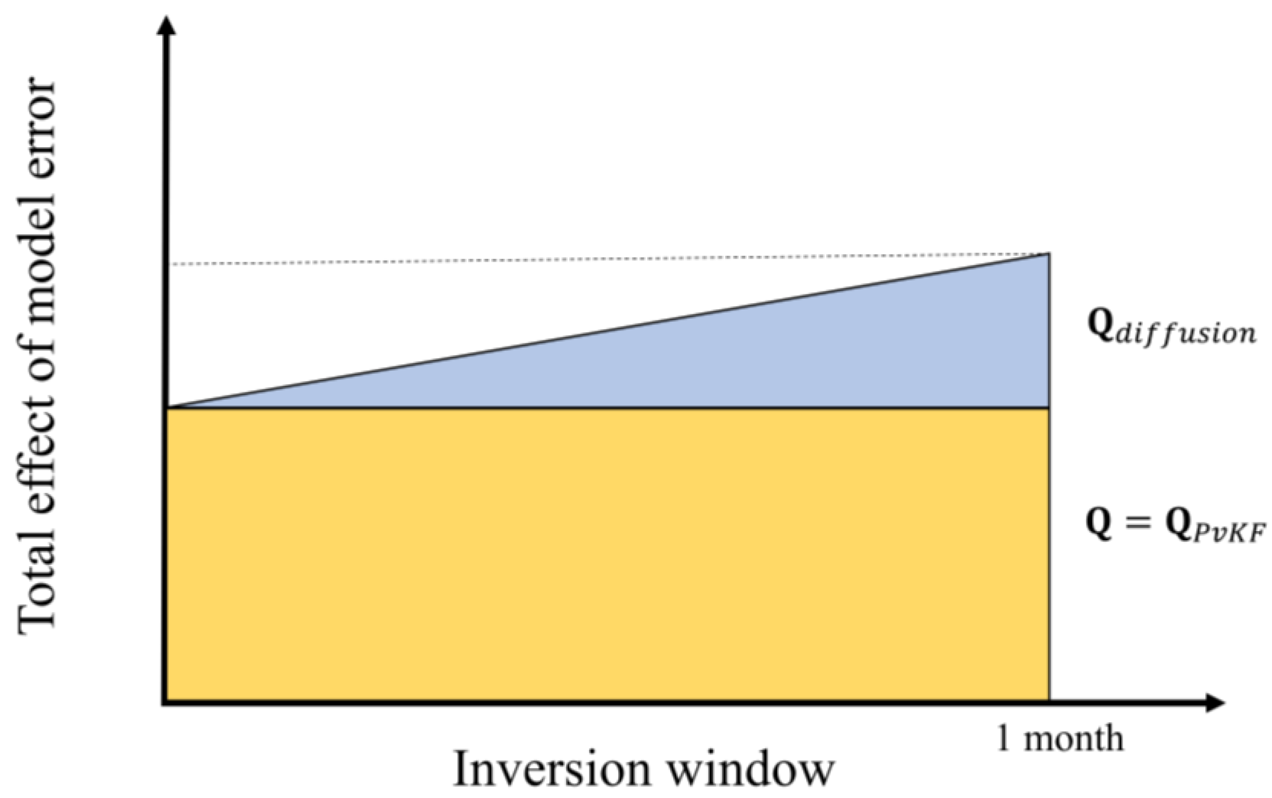
4.2. Implications for Model Error

Model propagated error, P f ( A 1 , Q ) in Equation (7), not only depends on the error covariance of the initial state but can also be produced due to imperfections in the model. We recall that for practical purposes, our inversions neither rely on a perfectly known initial state nor a perfect CTM. We integrate a PvKF formulation that can cost-effectively provide that error information on the initial state and the model (see Section 2.3). Furthermore, as shown earlier in Section 3.1, Section 3.2 and Section 3.3, accounting for those errors during the inversion process can improve emissions estimations; hence, it is important to understand the causes of those improvements.
Using the PvKF assimilation, we obtain the optimal estimation of the analysis error covariance ( A ) that is used to initialize the propagation of errors during the inversion. Propagation of this error covariance ( H o P t f ( A 1 ) H o   T ) is the key element in forming correlations that exist by nature in the model space but are often missed in a typical 4D-Var inversion (see Appendix A, Figure A1); thus, not accounting for this error may cause significant degradation of the inversion results (see Section 3).
Nevertheless, the entire error during inversion does not necessarily originate from the initial state, but may also be formed by the model, given that the model is not perfect. As in any Kalman filter, the PvKF does not depend on a perfect model assumption and thus allows for the inclusion of the model error during the inversion window. Contrary to the model propagation of the initial analysis error covariance ( H o P t f ( A 1 ) H o   T ), which involves the finer structure of the model background correlations, modelling error covariance ( Q ) is assumed to be proportional to the field due to a lack of information about its shape. In fact, there is little knowledge about the underlying processes driving model error covariance Q [18,25].
The origin of Q is generally unknown, so that identifying its underlying structure is almost implausible [75]. It has been shown in previous studies as well as here that the effect of model error is not negligible [25,78], while there are several explanations of their causes. In this study, the effect of adding model error can be explained in two ways, based on their forms and effects (although its origin remains unknown). The first type is a domain-wide stationery (bulk) error associated with various modelling characteristics. Using criteria based on innovation variance consistency in PvKF assimilation according to Voshtani et al., 2022b [38], we obtain the estimated value of the corresponding model error covariance Q , hereafter referred to as Q P v K F , which is used in our OSSE experiments (i.e., Q = Q P v K F ). Note that numerical discretization error was identified as the first source of error to be associated with the need for Q [61,79,80,81,82,83]. In particular, Menard et al., 2021 [82] argue that although we rely on the continuous behaviour of the linear advection, a discretized scheme used in the model can lead to a loss of total variance. Therefore, part of this bulk model error tends to compensate for that loss. Here in this section, we discuss the actual model error, which may be caused by neglecting the explicit diffusion of the model.
The model error can also be produced due to assumptions employed in our inversion/assimilation system. For example, here, the propagation of the error during inversion/assimilation is performed using a continuous formulation based on the advection of variance. It has been shown previously that over the 3-day revisit time of GOSAT the total variance remains conserved to a great extent (>95%) [34]. Relying on that assumption for a month of inversion in our experiments may lead to a degradation in realistically simulating the forecast model error. In fact, for the extended period of a month, diffusion spreads a portion of the variance in the form of spatial correlation, which is not considered in error propagation formulation based on the advection-only scheme used in PvKF. Those missing correlations might be addressed using a general form of parametric Kalman filter [81], where besides the variance, the evolution of characteristic parameters of correlations are computed, yet at a sizeable additional cost. Nevertheless, using a simple form of model error, we can compensate for the missing correlations due to diffusion by approximating its impact on the model concentrations. In Appendix B, we present a simple approach to approximate the violation of diffusion assumption that appears in the form of modelling error ( Q d i f f u s i o n ). We found an almost linear growth of this type of error over time. Therefore, the actual modelling error can be derived from a relationship as Q = Q P v K F + Q d i f f u s i o n . Figure 8 shows a schematic view of the estimated modelling error ( Q P v K F ) over time that is compounded by the approximated modelling error due to neglecting diffusion.

4.3. Computational Timing of Inversions

We showed earlier in our OSSE results in Section 3 that both the initial analysis field and model-propagated analysis error covariance can substantially impact inversion results in reproducing the true emissions. This section examines the computational time required for our modified inversion schemes that link PvKF assimilation to 4D-Var inversion. We recall that the 4D-Var inversion is designed in a way that the estimation iteratively converges to a local minimum (considered as an optimal solution) by minimizing a quadratic cost function ( J ) of the residuals between the model and observations (Equation (3)). It is also assumed that when the reduction of the cost function between successive iterations is less than 1%, the iteration process will be terminated (see Section 3.2). Using consistent convergence criteria for all experiments, we compare the computational time of employing different cost functions (Type 0–3 inversions or Equations (7)–(10)) in terms of the required iterations. Accordingly, Figure 9a depicts the value of the cost functions J at each iteration until convergence for all types of inversions. Note that the results here are associated with the OSSE of non-uniform perturbations, as described in Section 3.3, Figure 6.
Our results in Figure 9a indicate that performing Type 1 inversions with a biased model forecast initial and assuming a perfectly known state of the model (light blue line) requires 23 iterations for convergence. However, only accounting for an improved initial field (red line) from our optimal PvKF analysis ( c i a ) significantly reduces the computational cost of inversion. In fact, the number of iterations reaches nine in Type 2 (~one-third compared to the cost of Type 1). Now, once the model-propagated error covariance ( H o P f ( A 1 ) H o   T ) is also considered in our cost function of Type 3 (purple line), the number of iterations for convergence reaches eight, indicating that the cost of inversion does not change significantly. A similar effect is observed when the model error is considered (green line) in our cost function Type 0 ( H o P f ( A 1 , Q ) H o   T ), and the number of iterations remains the same. These comparisons imply that although accounting for the propagation of error covariance, either from imperfect transport or the initial state, does not provide a noticeable computational benefit, it exerts a substantial impact on the quality of the posterior emissions (e.g., see Table 3). On the other hand, considering the optimal initial analysis field maintains not only a better emissions constraint but also a lower cost of inversion. Note that the PvKF before the inversion window is computationally inexpensive, as it requires a little more than two model runs [34]. Hence, the overall cost of inversion combined with the PvKF assimilation remains low enough compared to the cost of Type 1 inversion (without PvKF assimilation).
Consistent with the experiments in Section 3, in Figure 9a we only look at the marginal difference in adding improved error statistics to the inversion once the initial state has already been corrected with assimilation analysis. Now, in another experiment, we keep the initial field of the model forecast and replace only the error covariance term in the cost function (Figure 9b). In fact, during the assimilation window, besides the model forecast ( c f ), we account for the model propagation of error covariance without updating them by observation assimilation. Accordingly, at the end of the assimilation window, instead of the analysis error covariance matrix A 1 , we obtain the forecast error covariance P 1 sto initialize the inversion. In addition, an updated form of model error ( Q ), as described in Section 4.2, is used in this experiment. Therefore, we can test if the error statistics alone (due to initial or model transport) are sufficient to reduce the computational cost.
Figure 9b presents three forms of inversions, all of which carry on the same model forecast ( c f ). Besides the Type 1 baseline inversion (light blue line), the figure shows an inversion (dark blue line) where the model-propagated forecast error is considered ( H o P f ( P 1 ) H o   T ), and another inversion (grey line) where model error is added to the forecast error ( H o P f ( P 1 , Q ) H o   T ). The results of the computational cost of inversions indicate that accounting for those error covariances in the cost function can reduce the number of iterations to 20 and 18, respectively. It suggests that the effect of error statistics alone would barely reduce the computational cost (up to ~20%). Although this amount is greater than the cost of the marginal difference of adding error statistics once the analysis is already used as the initial field (~10% reduction in cost; Figure 9a), it is still insignificant compared to the cost of replacing the initial forecast field by the analysis (~65% reduction). Note that the effect of error statistics alone (given the same c f ) on recovering the spatial distribution of true emissions is also more significant than the marginal effect of adding those errors when the analysis field is used. Finally, we remark that using the updated form of model error ( Q ) than the initial form ( Q ) provides no further reduction of the computational time of inversion (see Figure S4).

5. Summary and Conclusions

We present a new approach for performing methane source estimation, where the PvKF assimilation system of methane concentrations is combined with the 4D-Var source inversion. Previous methane inversion studies typically assume that the initial state uncertainties are negligible compared to the effect of accumulated emissions uncertainties for a typical duration of methane inversion (e.g., one month) in a limited domain. As a result, the state is considered to be close to the truth, and thus the inversion is nearly insensitive to the initial state uncertainties. However, in this study, we not only produce an assimilation analysis with small uncertainties to initialize the 4D-Var inversion but also account for those state uncertainties for the duration of the inversion. Our PvKF assimilation scheme provides this information. It is a lightweight assimilation system that allows for the propagation of errors using an advection scheme while remaining capable of taking the model error approximation into account. These state estimation properties allow us to examine their effect on the source estimation when it is linked to an inversion system.
It is also commonly assumed in methane inversion studies that errors in observation space are not correlated (or correlations are insignificant), and thus independent measurement errors dominate the total error weight, resulting in a diagonal observation error covariance. This assumption is indirectly attributed to the perfect model assumption made in many methane inversion studies. However, in our proposed assimilation–inversion system, the effect of the model forecast errors in the observation space leads to a non-diagonal error covariance matrix. This covariance matrix aims to provide proper correlations when the state of the system is not considered perfect, which is the case in reality. Accordingly, besides the impact of the initial analysis field provided by our PvKF assimilation, we examine the influence of forecast error covariance (model-propagated initial error and modelling error) on the inversion results.
We demonstrate observing system simulation experiments (OSSEs) to achieve our goals using the hemispheric CMAQ model and simulated GOSAT methane observations. Our source estimation system considers a monthly mean correction on methane emissions at the grid level across the domain. We construct modified inversion cost functions to account for those state characteristics, including (i) the effect of the optimal initial analysis field, (ii) the forecast of analysis error covariance, and (iii) the approximated modelling error, in reproducing true emissions. In addition, different perturbations of prior methane emissions, including (i) uniform perturbations of all sectors together, (ii) individual sectoral perturbations, and (iii) non-uniform perturbations, are generated to address the limitation of a typical 4D-Var inversion that relies on perfect state assumptions and a diagonal observation error covariance.
Our base case OSSE with uniform perturbation of total methane emissions indicates that not only the initial analysis concentrations but their model-propagated uncertainties have a substantial impact on recovering the true emissions. Comparing the proposed modified inversion cost function, which is fully linked to the assimilation of state and uncertainty (Type 0), with the regular cost function that only relies on the (biased) model forecast with the perfect assumption (Type 1) shows a considerable improvement in posterior emissions statistics. As a result, NMB and NME indicate 37% and 51% reduction while the correlation R increases from 0.88 to 0.98. In addition, using a biased initial state (model forecast with perfect model assumption instead of assimilation analysis) results in a significant overestimation of posterior emissions in many regions with large sources. Accounting for the initial analysis field instead of forecast concentrations improves inversion results but still remains inaccurate, particularly over the large local sources. However, including the model-propagation analysis uncertainty can significantly improve emissions constraints over those areas. This is mainly due to the structures of the error correlations that exist in the model forecast but are usually ignored by making perfect model assumptions in 4D-Var inversion. We also found that by accounting for the estimated model error Q , in addition to the analysis field and model propagation of uncertainties, slight overall improvements are obtained for the posterior emissions. This impact is more effective in areas where the density of observations is smaller, suggesting that added model error Q makes those observations more impactful in recovering the true emissions.
Our results using individual sectoral perturbation also emphasize the importance of considering both the analysis field and model propagation of errors for each sectoral inversion experiment. Nevertheless, the analysis field reflects a more tangible impact on improving local (or point) sources, such as those in the energy sector, while the influence of the model error propagation is more substantial on area sources, such as those in the agriculture sector. In addition, when the initial state is biased or when the model is assumed to be perfect, inversion with only one sector perturbation can negatively impact the posterior emissions of other sectors, which were initially unperturbed. This effect is also resolved when we use the initial analysis together with model-propagated uncertainties (Type 0). Finally, variable perturbations of different sectors together (a more realistic case) are examined in our OSSE experiments. The results overall go along with our previous finding with uniform perturbations, indicating 20% and 32% decreases in NMB and NME, respectively, and an increase from 0.90 to 0.99 in R.
The computational timing of using different inversion cost functions is also examined. Using a modified form of 4D-Var inversion, as proposed in this study (Type 0), suggests a significant reduction (of more than 60%) in the computational cost of inversion. This reduction occurs mainly when the optimal analysis initial field from PvKF assimilation, instead of the biased model forecast, is used. On the other hand, the propagation of analysis errors (and transport errors) in our OSSE experiment (Type 3 and Type 0) shows a negligible improvement in the computational time of inversion (10–20% reduction). An implication for the computational benefit of the 4D-Var inversion with optimal analysis is that the initial state is the closest to the truth, so that inversion requires fewer iterations to converge. In other words, the optimal analysis field avoids the additional iterations that 4D-Var inversion might use to compensate for the bias in the model forecast initial. Those additional iterations may appear in the case of not providing the optimal analysis field, even though a more realistic error covariance is taken into account in the cost function.
One main limitation of this modified 4D-Var source estimation, despite its practical application as well as high computational efficiency, exists in the simplified assumptions for simulating and evolving errors. In fact, using an advection-only scheme for propagating errors over a month-long inversion window may cause a loss of variance, which eventually can impact our ability to constrain emissions with our inversion system. Although we can partially compensate for that loss by using an extra modelling error in a simple form (see Section 4.2), a more precise solution for an extended period of inversion is to account for that loss by propagating the correlations using a diffusion scheme together with the advection of variance. This, however, entails extra computational costs.
Another limitation of the current approach that can be resolved in the future is associated with the simple form of model error, Q . We assumed a fairly primitive form of the model error, which is spatially proportional to the methane variance field; however, this leads to inadequate correction for the energy and waste sector, contrary to the agriculture and wetlands. Thus, the structure of the model error can be designed to be more sophisticated in the future to address emissions inversions of large and local sources, such as those in the energy and waste sectors.
Finally, the proposed source estimation framework provides a practical application for real observations of different types to address the limitations of similar inverse modelling and to improve the current inventories. However, the current method is yet capable of estimating the error statistics of the emissions. To efficiently provide that information using the current source estimation approach, we need to develop a coupled source–state estimation system with joint assimilation–inversion capabilities in the future. This allows one to propagate the emissions error besides the state error and estimate their uncertainties as part of the solution.

Supplementary Materials

The following supporting information can be downloaded at: https://www.mdpi.com/article/10.3390/atmos14040758/s1, Figure S1: Given the cost function of Equation (7) in the main manuscript, the prior and observation term of the cost function has the form J b = 1 2 ( x x b ) T B 1 ( x x b ) and J o = t = 0 n 1 2 y t o H t ( c 1 a , x ) T H o P t f ( A 1 , Q ) H o   T + R t 1 y t o H t ( c 1 a , x ) , respectively. (a) Show a traditional method of estimating γ that minimizes the sum of a normalized cost function [67]. J 0 is the magnitude of the total cost function ( J = γ J b + J o ) once γ = 0, indicating an optimization without prior constraint; and J 1 e 6 is the magnitude of the total cost function at γ = 106, showing an optimization with a dominant prior constraint. In this method, we aim at a γ among a few selected values that minimize the total normalized error. It shows that γ = 900 is the appropriate choice, although, for a wider range of this parameter (e.g., 500–2000), the choice of γ has little impact on the overall optimization (inversion) solution. (b) The L-curve method for the determination of the regularization parameter shows a comparison between the prior term of the cost function ( J b ) in the y-axis and the observation term of the cost function ( J o ) in the x-axis for different choices of γ . According to the method of Hansen (1999) [70], γ = 900 is an optimal (balanced) choice for the regularization parameter. In principle, the optimal γ is obtained when the solution tends to change in nature from being dominated by the prior cost (or perturbation error, where a small variation of γ causes rapid changes in J b ) to being dominated by the observation cost (or regularization/smoothing error where a large variation of γ makes a slow improvement in J b ); Figure S2: (a–e) statistical comparison of the prior and posterior emissions against true emissions in scatter plots for the only perturbed agriculture sector, (f–j) only perturbed energy sector, (k–o) only perturbed waste sector, and (p–t) only perturbed wetland sector. The prior emissions are generated using 50% uniform perturbation of each sector individually; Figure S3: (a) the prior–true emissions (±25–50% variable perturbation); (b) posterior–true emissions in Type 0 inversion using analysis initial ( c 1 a ) and both observation R and model-propagated analysis error covariance H o P t f ( A 1 , Q ) H o   T ; (c) posterior–true emissions in Type 1 inversion using forecast initial ( c 1 f ) and observation error covariance R, (d) posterior–true emissions in Type 2 inversion using analysis initial ( c 1 a ) and observation error covariance R; € posterior–true emissions in Type 3 inversion using analysis initial ( c 1 a ) and both observation R and model-propagated analysis error covariance H o P t f ( A 1 ) H o   T , but with no model error. Statistical comparison of the (f) the prior emissions and (g–j) posterior emissions of Type 0–3 inversion, respectively. x-axis and y-axis represent the true and the prior/posterior emissions, respectively. In (f–j), P f ( A 1 , Q ) is shown as P , and P f ( A 1 ) is shown as P . Synthetic observations are generated using the nature run initialized by the analysis, and a 2-week spin-up is used for the initialization; Figure S4: Comparison between the computational cost of two inversions in which only model error is different in the cost function. Q is the updated form of model error ( Q = Q + Q d i f f u s i o n ). Q is the estimated model error during the PvKF assimilation (or Q P v K F ) and Q d i f f u s i o n is approximated model error due to neglecting propagation of error correlations by diffusion; Figure S5: Normalized difference of concentrations between two cases where in the first one, the model diffusion scheme is deactivated, and in the second one, it is activated. It shows the distribution at the model’s first layer after one month of simulation. Except for this difference, all other inputs and configurations between the two cases are the same.

Author Contributions

Conceptualization, S.V., R.M., T.W.W. and A.H.; methodology, S.V. and R.M.; software, S.V.; formal analysis, S.V. and T.W.W.; investigation, S.V.; writing—original draft preparation, S.V.; writing—review and editing, R.M., T.W.W. and A.H.; visualization, S.V.; supervision, R.M., T.W.W. and A.H. All authors have read and agreed to the published version of the manuscript.

Funding

This research received no external funding.

Institutional Review Board Statement

Not applicable.

Informed Consent Statement

Not applicable.

Data Availability Statement

The GOSAT satellite data are available from the European Space Agency Greenhouse Gases Climate Change Initiative at http://cci.esa.int/ghg (last access: 31 August 2022). EDGAR v6 anthropogenic emission inventories are available at https://edgar.jrc.ec.europa.eu/dataset_ghg60 (European Commission, 2021), accessed on 31 August 2022. The source code for PvKF assimilation is accessible through https://github.com/Sinavo/PvKF_crv_methane.git. The CMAQ Adjoint model is available from https://github.com/usepa/cmaq_adjoint. Modelling data can be accessed by contacting the corresponding author: Sina Voshtani (SinaVoshtani@cmail.carleton.ca).

Acknowledgments

The authors of this paper acknowledge the free use of methane emissions data from the Emissions Database for Global Atmospheric Research (EDGAR) (https://edgar.jrc.ec.europa.eu/index.php/dataset_ghg60). Simulations for this study were performed in part by computational resources provided by Compute Canada (http://www.computecanada.ca).

Conflicts of Interest

The authors declare no conflict of interest.

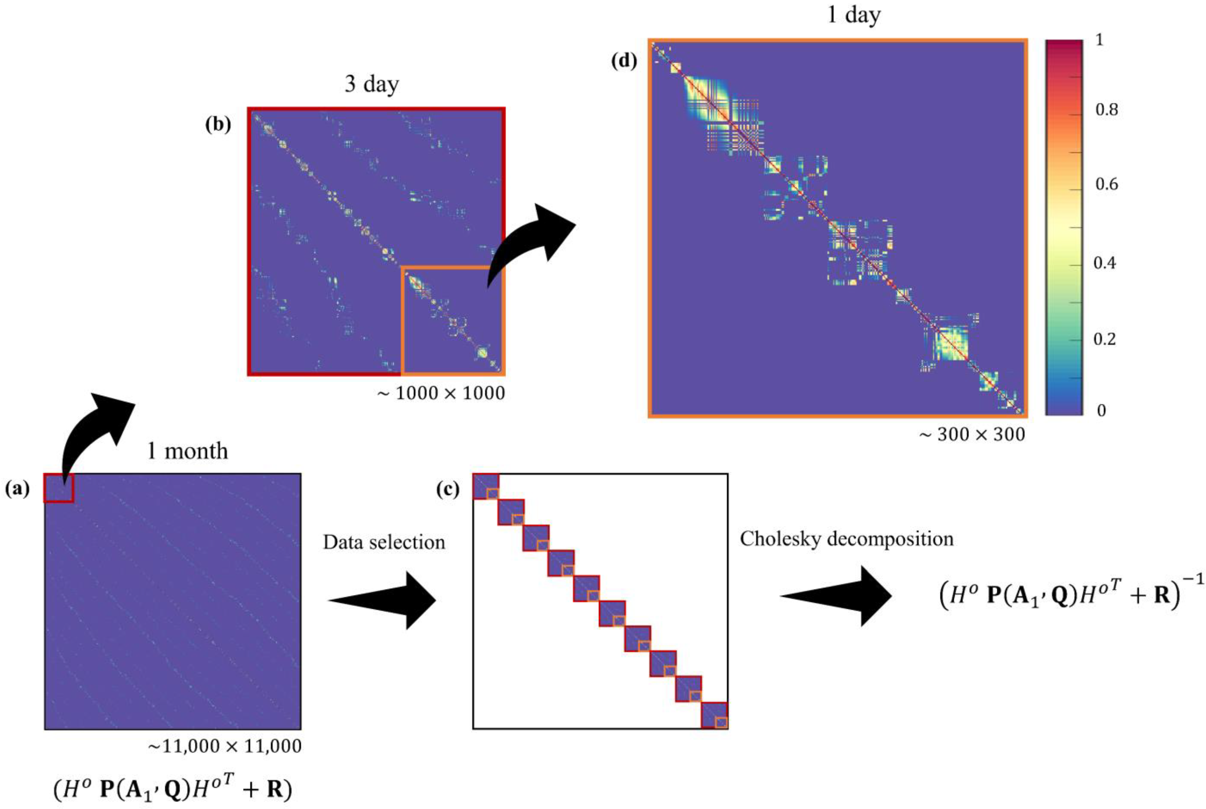
Appendix A. Numerical Aspects of Matrix Inversion

We use GOSAT methane observations for a period of a month, which contains 11,489 observations after all quality control and bias removal. It is typically assumed in methane inversion studies that the observation errors of this type are uncorrelated (or with insignificant correlations) both in space and time, resulting in a diagonal observation error covariance (R) [19,25,30,40,42]. Contrary to the observation error covariance, the forecast error covariance in observation space ( H o P f H o   T ) is not diagonal (Equation (7)). From a physical point of view, since the forecast error is propagated in time and space, its error covariance mapped into a one-month-long observation space is no longer a diagonal matrix (in observation space). To make this clearer, the elements of the 11,489 × 11,489 covariance matrix (i.e., H o P f H o   T + R ) are, in fact, ordered by observation ID numbers (not by time and not with space). Therefore, the forecast error correlates with different ID numbers (or observation space), resulting in a covariance matrix, H o P f H o   T + R , that is not a diagonal matrix for a month-long data window. In contrast, if we would only account for observation errors that are spatially and temporally uncorrelated, it would lead to a diagonal matrix in the observation space.
Since the number of observations is significant, as is the case here, inverting the covariance matrix, H o P f H o   T + R , becomes problematic. For regular matrices of that size (i.e., non-diagonal, non-sparse), the matrix inversion is not only computationally expensive but could lead to numerical issues [84].
In data assimilation, a traditional approach known as the data selection procedure [72,85,86] is used to avoid inverting large covariance matrices in observation space, H o P f H o   T + R . The data selection procedure involves partitioning the entire set of observations into smaller sets, known as batches of observations, that are mutually uncorrelated (also referred to as observation packets by Rodgers, 2000 [87]). In this case, the sizeable non-diagonal observation error covariance matrix transforms into a block diagonal matrix (with a reasonable block dimension), where each block represents the corresponding batch of observations (Figure A1).
Figure A1. (a) One-month non-diagonal error covariance, H o P f H o   T + R , is applied to the data selection procedure with (b) 3 days batch of observations to form (c) a block diagonal matrix of the same size. (d) Non-diagonal covariance matrix in one day.
Atmosphere 14 00758 g0a1
In data selection, in general, we divide the model domain into N regions and perform the analysis for each region. By limiting the number of observations (p) that influence analysis in a given region (e.g., p  < 1000), the size of the error covariance matrix to invert will be reduced (i.e., p  × p) and thus be manageable. The influence of observations on a region is determined by the correlation length scale. For example, any observation that is farther than five times the correlation length will not contribute to the analysis equation of the corresponding region. Thus, the number of regions to consider depends on the correlation length scale and the maximum number of observations that we can process in matrix inversion. This procedure is typical for optimal interpolation (OI) [72]. Note that some variants of this scheme (not discussed here) are also designed for the ensemble Kalman filter [85,88].
In the case of GOSAT satellite observations, each observation in space is considered with its own time (i.e., satellite retrieval time). Thus, it is more appropriate to partition the GOSAT observations according to their retrieval times, meaning that the error correlations between two observations depend not only on their geographical distance but also on their time difference. In this study, we simply assume that there are no correlations after three days between two locations of observations. As shown in Figure A1, we conduct a data selection procedure by considering a 3-day batch of GOSAT observations equivalent to the satellite revisit time. In this case, the number of observations within a batch remains as low as about 1000. Note that for a larger number of observations (p  1500 herein), the condition number of the covariance matrix increases rapidly, resulting in a non-full rank matrix.
Figure A1a displays the full error covariance matrix for a period of a month (and of a size ~11,000 × ~11,000). Ignoring the small covariances between the 3-day batches results in a block diagonal matrix (Figure A1c). Each block is represented in Figure A1b, where we perform matrix inversion using the Cholesky decomposition [89] to solve a system of linear equations of the same size as in that block. In Figure A1d, the covariance elements are shown within a day and are normalized relative to the values in the main diagonal. The correlation structures (off-diagonal elements) in this figure retain values that are as substantial as the main diagonal. Figure A1b indicates that the sub-diagonal elements (i.e., non-zero values that run parallel to the main diagonal) are from observations that occur one day (for the closest sub-diagonal line) or two days (for the second sub-diagonal line) later, but at slightly different locations. It implies that observations in a subsequent day are being translated into space according to the 3-day revisit cycle of GOSAT, but because of accounting for correlations using H o P f H o   T , they appear as non-zero correlations, although R remains diagonal.

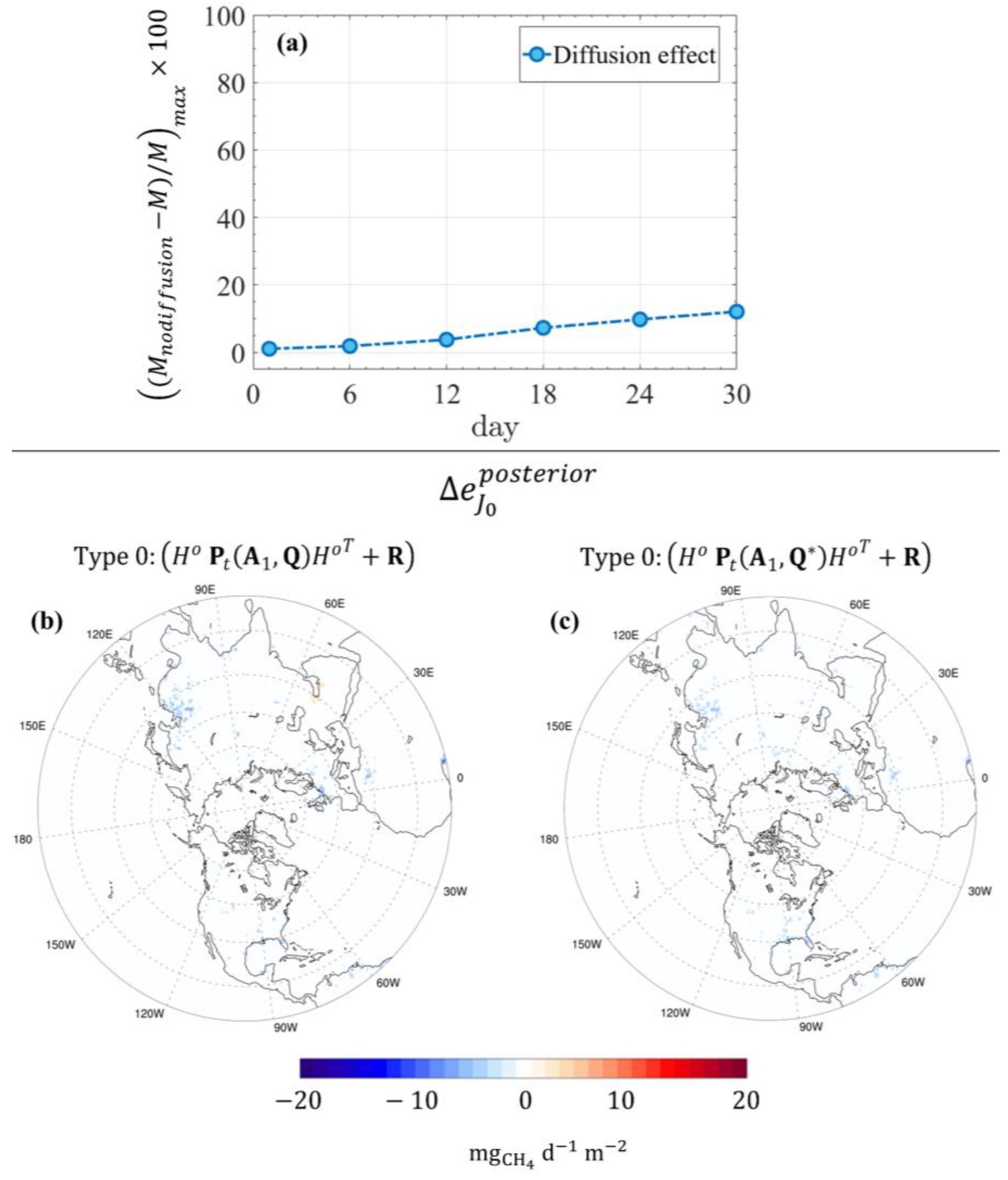
Appendix B. Approximation of Modelling Error Due to Violation of Diffusion

We perform a series of model forecast simulation experiments to determine how the forecast error variance remains conserved after a month of integration. We approximate the evolution of error variance as proportional to model forecast concentrations while considering the model with an active or deactivated diffusion scheme. Our results indicate that a maximum of 12% violation of the innovation covariance consistency occurs after one month if we do not account for the model error covariance Q (Figure A2a). Figure S5 also shows the map of methane concentrations of that difference in the first layer of the model after one month. We consider this effect (unaccounted diffusion of error variance) on the forecast error covariance as the modelling error due to the diffusion ( Q d i f f u s i o n ). Thus, it is recommended to include Q d i f f u s i o n for the extended period of error propagation (e.g., Δ T one month) using the PvKF advection-only scheme. We also found an approximately linear behaviour of this effect on the total model error, as shown in Figure A2a. To compare Q d i f f u s i o n with the model error covariance that is already estimated ( Q P v K F ), we perform the same procedure to retain its impact on domain concentrations over the same month of integration. Our results indicate that the effect of Q P v K F is nearly two times larger than the effect of Q d i f f u s i o n at the end of a month-long simulation.
To test the effect of Q d i f f u s i o n on emissions inversion results, we assume a simple form of that error (Figure A2b) as explained above (proportional to the field with linear growth over time). We repeat our OSSE experiment in Section 3.3 with the same inputs and configuration, except that the model error covariance Q is replaced with Q in Type 0 inversion (see Table 2). Besides the estimated model errors ( Q P v K F ), Q includes model error covariance due to the violation of diffusion ( Q d i f f u s i o n ); thus, Q = Q P v K F + Q d i f f u s i o n . Figure A2b,c compares the spatial distribution of posterior–true emissions for two inversion cases: (i) with Q = Q P v K F and (ii) with Q . The result shows a similar spatial distribution of posterior emissions with minor changes in magnitude over some large emissions areas. It implies that the additional part of the model error covariance due to diffusion ( Q d i f f u s i o n ) has a rather small impact on recovering true emissions, although it was shown in Section 3.3 that removing the entire model error covariance can exert a substantial impact on the inversion results.
Figure A2. (a) Diffusion effect of model error ( Q d i f f u s i o n ) estimated using a series of forecast simulations. Comparison between posterior–true emissions of Type 1 of Section 3.3 (based on ± 25–50% non-uniform perturbation) where (b) uses model error covariance Q = Q P v K F and (c) uses model error covariance Q = Q P v K F + Q d i f f u s i o n .
Atmosphere 14 00758 g0a2

References

  1. Staniaszek, Z.; Griffiths, P.T.; Folberth, G.A.; O’Connor, F.M.; Abraham, N.L.; Archibald, A.T. The role of future anthropogenic methane emissions in air quality and climate. Npj Clim. Atmos. Sci. 2022, 5, 8. [Google Scholar] [CrossRef]
  2. Saunois, M.; Stavert, A.R.; Poulter, B.; Bousquet, P.; Canadell, J.G.; Jackson, R.B.; Raymond, P.A.; Dlugokencky, E.J.; Houweling, S.; Patra, P.K.; et al. The Global Methane Budget 2000–2017. Earth Syst. Sci. Data 2020, 12, 1561–1623. [Google Scholar] [CrossRef]
  3. Nisbet, E.G.; Jones, A.E.; Pyle, J.A.; Skiba, U. Rising methane: Is there a methane emergency? Preface. Philos. Trans. R. Soc. A Math. Phys. Eng. Sci. 2022, 380, 4. [Google Scholar] [CrossRef] [PubMed]
  4. Worden, J.R.; Cusworth, D.H.; Qu, Z.; Yin, Y.; Zhang, Y.; Bloom, A.A.; Ma, S.; Byrne, B.K.; Scarpelli, T.; Maasakkers, J.D.; et al. The 2019 methane budget and uncertainties at 1° resolution and each country through Bayesian integration Of GOSAT total column methane data and a priori inventory estimates. Atmos. Chem. Phys. 2022, 22, 6811–6841. [Google Scholar] [CrossRef]
  5. Dlugokencky. NOAA/GML. 2022. Available online: www.esrl.noaa.gov/gmd/ccgg/trends_ch4/ (accessed on 31 August 2022).
  6. Minx, J.C.; Lamb, W.F.; Andrew, R.M.; Canadell, J.G.; Crippa, M.; Dobbeling, N.; Forster, P.M.; Guizzardi, D.; Olivier, J.; Peters, G.P.; et al. A comprehensive and synthetic dataset for global, regional, and national greenhouse gas emissions by sector 1970-2018 with an extension to 2019. Earth Syst. Sci. Data 2021, 13, 5213–5252. [Google Scholar] [CrossRef]
  7. Brasseur, G.P.; Jacob, D.J. Modeling of Atmospheric Chemistry; Cambridge University Press: New York, NY, USA, 2017; p. 606. [Google Scholar]
  8. Ganesan, A.L.; Schwietzke, S.; Poulter, B.; Arnold, T.; Lan, X.; Rigby, M.; Vogel, F.R.; van der Werf, G.R.; Janssens-Maenhout, G.; Boesch, H.; et al. Advancing Scientific Understanding of the Global Methane Budget in Support of the Paris Agreement. Glob. Biogeochem. Cycles 2019, 33, 1475–1512. [Google Scholar] [CrossRef]
  9. Palmer, P.I.; Feng, L.; Lunt, M.F.; Parker, R.J.; Bosch, H.; Lan, X.; Lorente, A.; Borsdorff, T. The added value of satellite observations of methane forunderstanding the contemporary methane budget. Philos. Trans. R. Soc. A Math. Phys. Eng. Sci. 2021, 379, 21. [Google Scholar] [CrossRef]
  10. Jacob, D.J.; Varon, D.J.; Cusworth, D.H.; Dennison, P.E.; Frankenberg, C.; Gautam, R.; Guanter, L.; Kelley, J.; McKeever, J.; Ott, L.E.; et al. Quantifying methane emissions from the global scale down to point sources using satellite observations of atmospheric methane. Atmos. Chem. Phys. Discuss. 2022, 2022, 9617–9646. [Google Scholar] [CrossRef]
  11. Dlugokencky, E.J.; Nisbet, E.G.; Fisher, R.; Lowry, D. Global atmospheric methane: Budget, changes and dangers. Philos. Trans. R. Soc. A Math. Phys. Eng. Sci. 2011, 369, 2058–2072. [Google Scholar] [CrossRef]
  12. Bergamaschi, P.; Karstens, U.; Manning, A.J.; Saunois, M.; Tsuruta, A.; Berchet, A.; Vermeulen, A.T.; Arnold, T.; Janssens-Maenhout, G.; Hammer, S.; et al. Inverse modelling of European CH4 emissions during 2006–2012 using different inverse models and reassessed atmospheric observations. Atmos. Chem. Phys. 2018, 18, 901–920. [Google Scholar] [CrossRef]
  13. Maasakkers, J.D.; Jacob, D.J.; Sulprizio, M.P.; Scarpelli, T.R.; Nesser, H.; Sheng, J.X.; Zhang, Y.Z.; Lu, X.; Bloom, A.A.; Bowman, K.W.; et al. 2010–2015 North American methane emissions, sectoral contributions, and trends: A high-resolution inversion of GOSAT observations of atmospheric methane. Atmos. Chem. Phys. 2021, 21, 4339–4356. [Google Scholar] [CrossRef]
  14. Houweling, S.; Bergamaschi, P.; Chevallier, F.; Heimann, M.; Kaminski, T.; Krol, M.; Michalak, A.M.; Patra, P. Global inverse modeling of CH4 sources and sinks: An overview of methods. Atmos. Chem. Phys. 2017, 17, 235–256. [Google Scholar] [CrossRef]
  15. Wecht, K.J.; Jacob, D.J.; Sulprizio, M.P.; Santoni, G.W.; Wofsy, S.C.; Parker, R.; Bosch, H.; Worden, J. Spatially resolving methane emissions in California: Constraints from the CalNex aircraft campaign and from present (GOSAT, TES) and future (TROPOMI, geostationary) satellite observations. Atmos. Chem. Phys. 2014, 14, 8173–8184. [Google Scholar] [CrossRef]
  16. Frankenberg, C.; Aben, I.; Bergamaschi, P.; Dlugokencky, E.J.; van Hees, R.; Houweling, S.; van der Meer, P.; Snel, R.; Tol, P. Global column-averaged methane mixing ratios from 2003 to 2009 as derived from SCIAMACHY: Trends and variability. J. Geophys. Res. Atmos. 2011, 116, 12. [Google Scholar] [CrossRef]
  17. Prather, M.J.; Zhua, X.; Strahan, S.E.; Steenrod, S.D.; Rodriguez, J.M. Quantifying errors in trace species transport modeling. Proc. Natl. Acad. Sci. USA 2008, 105, 19617–19621. [Google Scholar] [CrossRef] [PubMed]
  18. Locatelli, R.; Bousquet, P.; Saunois, M.; Chevallier, F.; Cressot, C. Sensitivity of the recent methane budget to LMDz sub-grid-scale physical parameterizations. Atmos. Chem. Phys. 2015, 15, 9765–9780. [Google Scholar] [CrossRef]
  19. Turner, A.J.; Jacob, D.J.; Benmergui, J.; Brandman, J.; White, L.; Randles, C.A. Assessing the capability of different satellite observing configurations to resolve the distribution of methane emissions at kilometer scales. Atmos. Chem. Phys. 2018, 18, 8265–8278. [Google Scholar] [CrossRef]
  20. Kopacz, M.; Jacob, D.J.; Fisher, J.A.; Logan, J.A.; Zhang, L.; Megretskaia, I.A.; Yantosca, R.M.; Singh, K.; Henze, D.K.; Burrows, J.P.; et al. Global estimates of CO sources with high resolution by adjoint inversion of multiple satellite datasets (MOPITT, AIRS, SCIAMACHY, TES). Atmos. Chem. Phys. 2010, 10, 855–876. [Google Scholar] [CrossRef]
  21. Janardanan, R.; Maksyutov, S.; Tsuruta, A.; Wang, F.J.; Tiwari, Y.K.; Valsala, V.; Ito, A.; Yoshida, Y.; Kaiser, J.W.; Janssens-Maenhout, G.; et al. Country-Scale Analysis of Methane Emissions with a High-Resolution Inverse Model Using GOSAT and Surface Observations. Remote Sens. 2020, 12, 375. [Google Scholar] [CrossRef]
  22. Lu, X.; Jacob, D.J.; Wang, H.L.; Maasakkers, J.D.; Zhang, Y.Z.; Scarpelli, T.R.; Shen, L.; Qu, Z.; Sulprizio, M.P.; Nesser, H.; et al. Methane emissions in the United States, Canada, and Mexico: Evaluation of national methane emission inventories and 2010–2017 sectoral trends by inverse analysis of in situ (GLOBALVIEWplus CH4 ObsPack) and satellite (GOSAT) atmospheric observations. Atmos. Chem. Phys. 2022, 22, 395–418. [Google Scholar] [CrossRef]
  23. Locatelli, R.; Bousquet, P.; Chevallier, F.; Fortems-Cheney, A.; Szopa, S.; Saunois, M.; Agusti-Panareda, A.; Bergmann, D.; Bian, H.; Cameron-Smith, P.; et al. Impact of transport model errors on the global and regional methane emissions estimated by inverse modelling. Atmos. Chem. Phys. 2013, 13, 9917–9937. [Google Scholar] [CrossRef]
  24. Saad, K.M.; Wunch, D.; Deutscher, N.M.; Griffith, D.W.T.; Hase, F.; De Maziere, M.; Notholt, J.; Pollard, D.F.; Roehl, C.M.; Schneider, M.; et al. Seasonal variability of stratospheric methane: Implications for constraining tropospheric methane budgets using total column observations. Atmos. Chem. Phys. 2016, 16, 14003–14024. [Google Scholar] [CrossRef]
  25. Stanevich, I.; Jones, D.B.A.; Strong, K.; Keller, M.; Henze, D.K.; Parker, R.J.; Boesch, H.; Wunch, D.; Notholt, J.; Petri, C.; et al. Characterizing model errors in chemical transport modeling of methane: Using GOSAT XCH4 data with weak-constraint four-dimensional variational data assimilation. Atmos. Chem. Phys. 2021, 21, 9545–9572. [Google Scholar] [CrossRef]
  26. Stanevich, I.; Jones, D.B.A.; Strong, K.; Parker, R.J.; Boesch, H.; Wunch, D.; Notholt, J.; Petri, C.; Warneke, T.; Sussmann, R.; et al. Characterizing model errors in chemical transport modeling of methane: Impact of model resolution in versions v9-02 of GEOS-Chem and v35j of its adjoint model. Geosci. Model Dev. 2020, 13, 3839–3862. [Google Scholar] [CrossRef]
  27. Tremolet, Y. Model-error estimation in 4D-Var. Q. J. R. Meteorol. Soc. 2007, 133, 1267–1280. [Google Scholar] [CrossRef]
  28. Tremolet, Y. Accounting for an imperfect model in 4D-Var. Q. J. R. Meteorol. Soc. 2006, 132, 3127. [Google Scholar] [CrossRef]
  29. Zhang, Y.; Jacob, D.J.; Maasakkers, J.D.; Sulprizio, M.P.; Sheng, J.-X.; Gautam, R.; Worden, J. Monitoring global tropospheric OH concentrations using satellite observations of atmospheric methane. Atmos. Meas. Technol. 2018, 18, 15959–15973. [Google Scholar] [CrossRef]
  30. Bousserez, N.; Henze, D.K.; Rooney, B.; Perkins, A.; Wecht, K.J.; Turner, A.J.; Natraj, V.; Worden, J.R. Constraints on methane emissions in North America from future geostationary remote-sensing measurements. Atmos. Chem. Phys. 2016, 16, 6175–6190. [Google Scholar] [CrossRef]
  31. Elbern, H.; Strunk, A.; Schmidt, H.; Talagrand, O. Emission rate and chemical state estimation by 4-dimensional variational inversion. Atmos. Chem. Phys. 2007, 7, 3749–3769. [Google Scholar] [CrossRef]
  32. Basu, S.; Guerlet, S.; Butz, A.; Houweling, S.; Hasekamp, O.; Aben, I.; Krummel, P.; Steele, P.; Langenfelds, R.; Torn, M.; et al. Global CO2 fluxes estimated from GOSAT retrievals of total column CO2. Atmos. Chem. Phys. 2013, 13, 8695–8717. [Google Scholar] [CrossRef]
  33. Deng, F.; Jones, D.B.A.; Henze, D.K.; Bousserez, N.; Bowman, K.W.; Fisher, J.B.; Nassar, R.; O’Dell, C.; Wunch, D.; Wennberg, P.O.; et al. Inferring regional sources and sinks of atmospheric CO2 from GOSAT XCO2 data. Atmos. Chem. Phys. 2014, 14, 3703–3727. [Google Scholar] [CrossRef]
  34. Voshtani, S.; Menard, R.; Walker, T.W.; Hakami, A. Assimilation of GOSAT Methane in the Hemispheric CMAQ.; Part I: Design of the Assimilation System. Remote Sens. 2022, 14, 371. [Google Scholar] [CrossRef]
  35. Pannekoucke, O.; Menard, R.; El Aabaribaoune, M.; Plu, M. A methodology to obtain model-error covariances due to the discretization scheme from the parametric Kalman filter perspective. Nonlinear Process. Geophys. 2021, 28, 1–22. [Google Scholar] [CrossRef]
  36. Skachko, S.; Menard, R.; Errera, Q.; Christophe, Y.; Chabrillat, S. EnKF and 4D-Var data assimilation with chemical transport model BASCOE (version 05.06). Geosci. Model Dev. 2016, 9, 2893–2908. [Google Scholar] [CrossRef]
  37. Skachko, S.; Errera, Q.; Menard, R.; Christophe, Y.; Chabrillat, S. Comparison of the ensemble Kalman filter and 4D-Var assimilation methods using a stratospheric tracer transport model. Geosci. Model Dev. 2014, 7, 1451–1465. [Google Scholar] [CrossRef]
  38. Voshtani, S.; Menard, R.; Walker, T.W.; Hakami, A. Assimilation of GOSAT Methane in the Hemispheric CMAQ; Part II: Results Using Optimal Error Statistics. Remote Sens. 2022, 14, 375. [Google Scholar] [CrossRef]
  39. Yu, X.Y.; Millet, D.B.; Henze, D.K. How well can inverse analyses of high-resolution satellite data resolve heterogeneous methane fluxes? Observing system simulation experiments with the GEOS-Chem adjoint model (v35). Geosci. Model Dev. 2021, 14, 7775–7793. [Google Scholar] [CrossRef]
  40. Zhang, Y.Z.; Jacob, D.J.; Lu, X.; Maasakkers, J.D.; Scarpelli, T.R.; Sheng, J.X.; Shen, L.; Qu, Z.; Sulprizio, M.P.; Chang, J.F.; et al. Attribution of the accelerating increase in atmospheric methane during 2010–2018 by inverse analysis of GOSAT observations. Atmos. Chem. Phys. 2021, 21, 3643–3666. [Google Scholar] [CrossRef]
  41. Turner, A.J.; Frankenberg, C.; Kort, E.A. Interpreting contemporary trends in atmospheric methane. Proc. Natl. Acad. Sci. USA 2019, 116, 2805–2813. [Google Scholar] [CrossRef]
  42. Turner, A.J.; Jacob, D.J.; Wecht, K.J.; Maasakkers, J.D.; Lundgren, E.; Andrews, A.E.; Biraud, S.C.; Boesch, H.; Bowman, K.W.; Deutscher, N.M.; et al. Estimating global and North American methane emissions with high spatial resolution using GOSAT satellite data. Atmos. Chem. Phys. 2015, 15, 7049–7069. [Google Scholar] [CrossRef]
  43. Bousserez, N.; Henze, D.K. Optimal and scalable methods to approximate the solutions of large-scale Bayesian problems: Theory and application to atmospheric inversion and data assimilation. Q. J. R. Meteorol. Soc. 2018, 144, 365–390. [Google Scholar] [CrossRef]
  44. Byun, D.; Schere, K.L. Review of the governing equations, computational algorithms, and other components of the models-3 Community Multiscale Air Quality (CMAQ) modeling system. Appl. Mech. Rev. 2006, 59, 51–77. [Google Scholar] [CrossRef]
  45. Alexe, M.; Bergamaschi, P.; Segers, A.; Detmers, R.; Butz, A.; Hasekamp, O.; Guerlet, S.; Parker, R.; Boesch, H.; Frankenberg, C.; et al. Inverse modelling of CH4 emissions for 2010–2011 using different satellite retrieval products from GOSAT and SCIAMACHY. Atmos. Chem. Phys. 2015, 15, 113–133. [Google Scholar] [CrossRef]
  46. Cressot, C.; Chevallier, F.; Bousquet, P.; Crevoisier, C.; Dlugokencky, E.J.; Fortems-Cheiney, A.; Frankenberg, C.; Parker, R.; Pison, I.; Scheepmaker, R.A.; et al. On the consistency between global and regional methane emissions inferred from SCIAMACHY, TANSO-FTS, IASI and surface measurements. Atmos. Chem. Phys. 2014, 14, 577–592. [Google Scholar] [CrossRef]
  47. Bergamaschi, P.; Houweling, S.; Segers, A.; Krol, M.; Frankenberg, C.; Scheepmaker, R.; Dlugokencky, E.; Wofsy, S.; Kort, E.; Sweeney, C. Atmospheric CH4 in the first decade of the 21st century: Inverse modeling analysis using SCIAMACHY satellite retrievals and NOAA surface measurements. J. Geophys. Res. Atmos. 2013, 118, 7350–7369. [Google Scholar] [CrossRef]
  48. Kuze, A.; Suto, H.; Nakajima, M.; Hamazaki, T. Thermal and near infrared sensor for carbon observation Fourier-transform spectrometer on the Greenhouse Gases Observing Satellite for greenhouse gases monitoring. Appl. Opt. 2009, 48, 6716–6733. [Google Scholar] [CrossRef]
  49. Butz, A.; Guerlet, S.; Hasekamp, O.; Schepers, D.; Galli, A.; Aben, I.; Frankenberg, C.; Hartmann, J.-M.; Tran, H.; Kuze, A.; et al. Toward accurate CO2 and CH4 observations from GOSAT. Geophys. Res. Lett. 2011, 38, 1–6. [Google Scholar] [CrossRef]
  50. Buchwitz, M.; Reuter, M.; Schneising, O.; Hewson, W.; Detmers, R.G.; Boesch, H.; Hasekamp, O.P.; Aben, I.; Bovensmann, H.; Burrows, J.P.; et al. Global satellite observations of column-averaged carbon dioxide and methane: The GHG-CCI XCO2 and XCH4 CRDP3 data set. Remote Sens. Environ. 2017, 203, 276–295. [Google Scholar] [CrossRef]
  51. Mathur, R.; Xing, J.; Gilliam, R.; Sarwar, G.; Hogrefe, C.; Pleim, J.; Pouliot, G.; Roselle, S.; Spero, T.L.; Wong, D.C.; et al. Extending the Community Multiscale Air Quality (CMAQ) modeling system to hemispheric scales: Overview of process considerations and initial applications. Atmos. Chem. Phys. 2017, 17, 12449–12474. [Google Scholar] [CrossRef]
  52. Olsen, E.; Fetzer, E.; Hulley, G.; Manning, E.; Blaisdell, J.; Iredell, L.; Susskind, J.; Warner, J.; Wei, Z.; Blackwell, W. AIRS/AMSU/HSB version 6 level 2 product user guide. USA NASA-JPL Technol. Rep. 2013, 1, 760. [Google Scholar]
  53. CMAQ Tutorials. Available online: https://www.epa.gov/cmaq/cmaq-documentation (accessed on 14 October 2021).
  54. Crippa, M.; Solazzo, E.; Huang, G.L.; Guizzardi, D.; Koffi, E.; Muntean, M.; Schieberle, C.; Friedrich, R.; Janssens-Maenhout, G. High resolution temporal profiles in the Emissions Database for Global Atmospheric Research. Sci. Data 2020, 7, 121. [Google Scholar] [CrossRef]
  55. Wang, F.J.; Maksyutov, S.; Tsuruta, A.; Janardanan, R.; Ito, A.; Sasakawa, M.; Machida, T.; Morino, I.; Yoshida, Y.; Kaiser, J.W.; et al. Methane Emission Estimates by the Global High-Resolution Inverse Model Using National Inventories. Remote Sens. 2019, 11, 2489. [Google Scholar] [CrossRef]
  56. Crippa, M.; Guizzardi, D.; Muntean, M.; Schaaf, E.; Lo Vullo, E.; Solazzo, E.; Monforti-Ferrario, F.; Olivier, J.; Vignati, E. EDGAR v6.0 Greenhouse Gas Emissions. Available online: http://data.europa.eu/89h/97a67d67-c62e-4826-b873-9d972c4f670b (accessed on 5 November 2021).
  57. Bloom, A.A.; Bowman, K.W.; Lee, M.; Turner, A.J.; Schroeder, R.; Worden, J.R.; Weidner, R.; McDonald, K.C.; Jacob, D.J. A global wetland methane emissions and uncertainty dataset for atmospheric chemical transport models (WetCHARTs version 1.0). Geosci. Model Dev. 2017, 10, 2141–2156. [Google Scholar] [CrossRef]
  58. UNC. Community Modeling and Analysis System CMAS [WWW Document]. SMOKE v3.6 User’s Man. Available online: https://www.cmascenter.org/smoke/ (accessed on 2 November 2021).
  59. IPCC. The Physical Science Basis; IPCC; Cambridge Univ Press: New York, NY, USA, 2013; p. 2013. [Google Scholar]
  60. Cohn, S.E. Dynamics of short-term univariate forecast error covariances. Mon. Weather Rev. 1993, 121, 3123–3149. [Google Scholar] [CrossRef]
  61. Menard, R.; Cohn, S.E.; Chang, L.P.; Lyster, P.M. Assimilation of stratospheric chemical tracer observations using a Kalman filter. Part I: Formulation. Mon. Weather Rev. 2000, 128, 2654–2671. [Google Scholar] [CrossRef]
  62. Menard, R.; Deshaies-Jacques, M. Evaluation of Analysis by Cross-Validation. Part I: Using Verification Metrics. Atmosphere 2018, 9, 86. [Google Scholar] [CrossRef]
  63. Hakami, A.; Henze, D.K.; Seinfeld, J.H.; Singh, K.; Sandu, A.; Kim, S.T.; Byun, D.W.; Li, Q.B. The adjoint of CMAQ. Environ. Sci. Technol. 2007, 41, 7807–7817. [Google Scholar] [CrossRef] [PubMed]
  64. Zhao, S.L.; Russell, M.G.; Hakami, A.; Capps, S.L.; Turner, M.D.; Henze, D.K.; Percell, P.B.; Resler, J.; Shen, H.; Russell, A.G.; et al. A multiphase CMAQ version 5.0 adjoint. Geosci. Model Dev. 2020, 13, 2925–2944. [Google Scholar] [CrossRef] [PubMed]
  65. Turner, M.D.; Henze, D.K.; Hakami, A.; Zhao, S.L.; Resler, J.; Carmichael, G.R.; Stanier, C.O.; Baek, J.; Sandu, A.; Russell, A.G.; et al. Differences Between Magnitudes and Health Impacts of BC Emissions Across the United States Using 12 km Scale Seasonal Source Apportionment. Environ. Sci. Technol. 2015, 49, 4362–4371. [Google Scholar] [CrossRef]
  66. Chen, Y.L.; Shen, H.Z.; Kaiser, J.; Hu, Y.T.; Capps, S.L.; Zhao, S.L.; Hakami, A.; Shih, J.S.; Pavur, G.K.; Turner, M.D.; et al. High-resolution hybrid inversion of IASI ammonia columns to constrain US ammonia emissions using the CMAQ adjoint model. Atmos. Chem. Phys. 2021, 21, 2067–2082. [Google Scholar] [CrossRef]
  67. Hakami, A.; Henze, D.K.; Seinfeld, J.H.; Chai, T.; Tang, Y.; Carmichael, G.R.; Sandu, A. Adjoint inverse modeling of black carbon during the Asian Pacific Regional Aerosol Characterization Experiment. J. Geophys. Res. Atmos. 2005, 110, 17. [Google Scholar] [CrossRef]
  68. Sandu, A.; Daescu, D.N.; Carmichael, G.R.; Chai, T.F. Adjoint sensitivity analysis of regional air quality models. J. Comput. Phys. 2005, 204, 222–252. [Google Scholar] [CrossRef]
  69. Byrd, R.H.; Lu, P.H.; Nocedal, J.; Zhu, C.Y. A limited memory algorithm for bound constrained optimization. SIAM J. Sci. Comput. 1995, 16, 1190–1208. [Google Scholar] [CrossRef]
  70. Hansen, P.C. The L-curve and its use in the numerical treatment of inverse problems. In Computational Inverse Problems in Electrocardiology; Johnston, P., Ed.; Advances in Computational Bioengineering Series; WIT: Boston, MA, USA, 2000; Volume 5, pp. 119–142. [Google Scholar]
  71. Bergamaschi, P.; Corazza, M.; Karstens, U.; Athanassiadou, M.; Thompson, R.L.; Pison, I.; Manning, A.J.; Bousquet, P.; Segers, A.; Vermeulen, A. Top-down estimates of European CH4 and N2O emissions based on four different inverse models. Atmos. Chem. Phys. 2015, 16, 715–736. [Google Scholar] [CrossRef]
  72. Lahoz, W.A.; Schneider, P. Data assimilation: Making sense of Earth Observation. Front. Environ. Sci. 2014, 2, 16. [Google Scholar] [CrossRef]
  73. Basu, S.; Lan, X.; Dlugokencky, E.; Michel, S.; Schwietzke, S.; Miller, J.B.; Bruhwiler, L.; Oh, Y.; Tans, P.P.; Apadula, F.; et al. Estimating Emissions of Methane Consistent with Atmospheric Measurements of Methane and δ13C of Methane. Atmos. Chem. Phys. Discuss. 2022, 2022, 15351–15377. [Google Scholar] [CrossRef]
  74. Wu, X.R.; Elbern, H.; Jacob, B. The assessment of potential observability for joint chemical states and emissions in atmospheric modelings. Stoch. Environ. Res. Risk Assess. 2022, 36, 1743–1760. [Google Scholar] [CrossRef]
  75. Tandeo, P.; Ailliot, P.; Bocquet, M.; Carrassi, A.; Miyoshi, T.; Pulido, M.; Zhen, Y.C. A Review of Innovation-Based Methods to Jointly Estimate Model and Observation Error Covariance Matrices in Ensemble Data Assimilation. Mon. Weather Rev. 2020, 148, 3973–3994. [Google Scholar] [CrossRef]
  76. Maasakkers, J.D.; Jacob, D.J.; Sulprizio, M.P.; Scarpelli, T.R.; Nesser, H.; Sheng, J.X.; Zhang, Y.Z.; Hersher, M.; Bloom, A.A.; Bowman, K.W.; et al. Global distribution of methane emissions, emission trends, and OH concentrations and trends inferred from an inversion of GOSAT satellite data for 2010–2015. Atmos. Chem. Phys. 2019, 19, 7859–7881. [Google Scholar] [CrossRef]
  77. Qu, Z.; Jacob, D.J.; Shen, L.; Lu, X.; Zhang, Y.Z.; Scarpelli, T.R.; Nesser, H.; Sulprizio, M.P.; Maasakkers, J.D.; Bloom, A.A.; et al. Global distribution of methane emissions: A comparative inverse analysis of observations from the TROPOMI and GOSAT satellite instruments. Atmos. Chem. Phys. 2021, 21, 14159–14175. [Google Scholar] [CrossRef]
  78. Orbe, C.; Waugh, D.W.; Yang, H.; Lamarque, J.F.; Tilmes, S.; Kinnison, D.E. Tropospheric transport differences between models using the same large-scale meteorological fields. Geophys. Res. Lett. 2017, 44, 1068–1078. [Google Scholar] [CrossRef]
  79. Daley, R. Estimating model-error covariances for application to atmospheric data assimilation. Mon. Weather Rev. 1992, 120, 1735–1746. [Google Scholar] [CrossRef]
  80. Daley, R. Estimating the wind-field from chemical-constituent observations—Experiments with a one-dimensional extended kalman filter. Mon. Weather Rev. 1995, 123, 181–198. [Google Scholar] [CrossRef]
  81. Pannekoucke, O.; Ricci, S.; Barthelemy, S.; Menard, R.; Thual, O. Parametric Kalman filter for chemical transport models. Tellus Ser. Dyn. Meteorol. Oceanogr. 2016, 68, 14. [Google Scholar] [CrossRef]
  82. Menard, R.; Skachko, S.; Pannekoucke, O. Numerical discretization causing error variance loss and the need for inflation. Q. J. R. Meteorol. Soc. 2021, 147, 3498–3520. [Google Scholar] [CrossRef]
  83. Gilpin, S.; Matsuo, T.; Cohn, S.E. Continuum Covariance Propagation for Understanding Variance Loss in Advective Systems. SIAM/ASA J. Uncertain. Quantif. 2022, 10, 886–914. [Google Scholar] [CrossRef]
  84. Strang, G.; Borre, K. Linear Algebra, Geodesy, and GPS; Wellesley-Cambridge Press: Wellesley, MA, USA, 1997. [Google Scholar]
  85. Houtekamer, P.L.; Mitchell, H.L. A sequential ensemble Kalman filter for atmospheric data assimilation. Mon. Weather Rev. 2001, 129, 123–137. [Google Scholar] [CrossRef]
  86. Cohn, S.E.; da Silva, A.; Guo, J.; Sienkiewicz, M.; Lamich, D. Assessing the effects of data selection with the DAO physical-space statistical analysis system. Mon. Weather Rev. 1998, 126, 2913–2926. [Google Scholar] [CrossRef]
  87. Rodgers, C.D. Inverse Methods for Atmospheric Sounding: Theory and Practice; World Scientific: Singapore, 2000; Volume 2. [Google Scholar]
  88. Migliorini, S. Information-based data selection for ensemble data assimilation. Q. J. R. Meteorol. Soc. 2013, 139, 2033–2054. [Google Scholar] [CrossRef]
  89. Krishnamoorthy, A.; Menon, D. Matrix inversion using Cholesky decomposition. In Proceedings of the 2013 Signal Processing: Algorithms, Architectures, Arrangements, and Applications (SPA), Poznan, Poland, 26–28 September 2013; pp. 70–72. [Google Scholar]
Figure 1. Schematic view of using the cost-efficient PvKF assimilation system for estimating methane emissions through 4D-Var inversion. Chemical Transport Model (CTM), PvKF Data Assimilation (DA), and 4D-Var Inverse Modelling (IM) systems are shown by grey arrows. ϵ q , ϵ o , and ϵ a represents model, observation, and analysis error, respectively.
Atmosphere 14 00758 g001
Figure 2. Sketch of the assimilation window in blue, followed by the inversion window in yellow, used in the proposed approach for estimating methane emissions. Depending on the assumptions, four types of experiments are shown to provide various initial fields and error covariances during the inversion window. * Experiment 4 represents what this study proposes and is equivalent to inversion Type 0 in Table 2. M denotes the CMAQ model and P f is model-propagated error covariance.
Atmosphere 14 00758 g002
Figure 3. Flowchart of the OSSE framework for optimizing methane emissions.
Atmosphere 14 00758 g003
Figure 4. (a) The prior–true emissions (+50% uniform perturbation); (b) the posterior–true emissions in Type 0 inversion using analysis initial ( c 1 a ) and both observation R and model-propagated analysis error covariance H o P t f ( A 1 , Q ) H o   T ; (c) the posterior–true emissions in Type 1 inversion using forecast initial ( c 1 f ) and observation error covariance R, (d) the posterior–true emissions in Type 2 inversion using analysis initial ( c 1 a ) and observation error covariance R; (e) the posterior–true emissions in Type 3 inversion using analysis initial ( c 1 a ) and both observation and model-propagated analysis error covariance H o P t f ( A 1 ) H o   T , but without model error. Statistical comparison of (f) the prior emissions and (gj) the posterior emissions of Type 0–3 inversions, respectively. The x-axis and y-axis represent the true and the prior/posterior emissions, respectively. In (fj), P f ( A 1 , Q ) is shown as P , and P f ( A 1 ) is shown as P . Simulated observations are generated using the nature run initialized by the analysis, and a 2-week spin-up is used for the initialization.
Atmosphere 14 00758 g004
Figure 5. (ae) The prior–true emissions and comparison of the posterior against the true emissions for the only perturbed agriculture sector, (fj) only perturbed energy sector, (ko) only perturbed waste sector, and (pt) only perturbed wetland sector. The prior emissions are generated using 50% uniform perturbation. Type 1 OSSE uses ( c 1 f ) and (R). Type 2 performs with analysis initial ( c 1 a ) and (R). Type 3 OSSE operates with analysis initial ( c 1 a ) and forecast of analysis error covariance ( H o P f ( A 1 ) H o   T ), and Type 0 OSSE works with analysis initial ( c 1 a ) and forecast of analysis error covariance with model error ( H o P f ( A 1 , Q ) H o   T ).
Atmosphere 14 00758 g005
Figure 6. (a) The prior–true emissions (±25–50% variable perturbation); the posterior–true emissions in (b) Type 0 inversion, (c) Type 1 inversion, (d) Type 2 inversion, and (e) Type 3 inversion. Statistical comparison of the (f) the prior emissions and (gj) posterior emissions of Type 0–3 inversions, respectively.
Atmosphere 14 00758 g006
Figure 7. (a) Total emissions of the truth, prior, and four types of posteriors (Type 0–3) associated with Case 1 inversion with uniform perturbation of total emissions; (b) total emissions of the truth, prior, and four types of posteriors (Type 0–3) associated with Case 6 inversion with non-uniform perturbation of total emissions.
Atmosphere 14 00758 g007
Figure 8. Schematic view of estimated part of the model error ( Q P v K F ) using an advection-only scheme in yellow, compared with an approximation of Q d i f f u s i o n in blue.
Atmosphere 14 00758 g008
Figure 9. (a) Comparison between the value of cost function against the number of iterations to show the required computational time of four different inversion types (Type 0–3); (b) Comparison between the computational time of inversions when the initial field is provided with the model forecast ( c i f ) for all the cases (Type 1 inversion); however, the impact of adding only error statistics to the cost function is shown.
Atmosphere 14 00758 g009
Table 1. Total daily mean methane emissions in four main sectors and their subsets. Anthropogenic emissions are based on EDGAR v6, and natural emissions are obtained from WetCHARTs v3.0 with the full ensemble mean.
AnthropogenicNatural
Agriculture
G g C H 4 d 1
Energy
G g C H 4 d 1
Waste
G g C H 4 d 1
Wetland
G g C H 4 d 1
386.42 (28.2%)303.65 (22.1%)196.9 (14.4%)483.81 (35.3%)
Agriculture Soil [93.830]
Agriculture waste burning [8.582]
Enteric fermentation a [249.04]
Manure management [34.96]
Aviation b (all types) [0.013]
Chemical process [0.526]
Combustion manufacturing [1.454]
Energy for building [28.247]
Fossil fuel fire [0.409]
Coal [89.05]
Gas [97.246]
Oil [73.233]
Iron-steel production [0.298]
Oil refineries [11.935]
Power industry [0.876]
Off-road [0.020]
Road transportation [0.175]
Shipping [0.167]
Solid waste incineration [33.997]
Solid waste c [74.114]
Water waste handling [88.79]
Wetland [483.81]
a Enteric fermentation and manure management represent the emissions of “livestock” used in similar inversion studies. b All types of aviation refer to three subsets in EDGAR v6, including aviation climb descent, aviation cruise, and aviation landing takeoff. c Solid waste is equivalent to landfills in similar studies.
Table 3. Normalized mean bias (NMB), Normalized mean error (NME), and Pearson’s correlation coefficient (R) for each perturbation case and inversion cost functions (Equations (7)–(10)). In cases 1–5, sector/sectors are all uniformly scaled up by 50%. In cases 6 and 7, sectors are perturbed non-uniformly between 25–50% (see Section 3.3 for the details).
Cost FunctionType 0:
J 0 ( c i a , P t f ( A 1 , Q ) , R )
Type 1:
J 1 ( c i f , R )
Type 2:
J 2 ( c i a , R )
Type 3:
J 3 ( c i a , P t f ( A 1 ) , R )
Perturbation NMBNMERNMBNMERNMBNMERNMBNMER
Case 1:
All sectors/Uniform
+0.020.060.98−0.390.570.88−0.110.290.94−0.030.100.97
Case 2:
Agriculture/Uniform
+0.010.040.99−0.070.280.96−0.050.120.930.000.060.95
Case 3:
Energy/Uniform
+0.030.030.98−0.180.310.95−0.090.220.94+0.030.030.97
Case 4:
Waste/Uniform
+0.020.020.99+0.110.450.94−0.030.100.95−0.020.030.98
Case 5:
Wetland/Uniform
−0.010.010.99−0.060.110.99−0.050.090.99−0.050.040.99
Case 6:
All sectors/Non-uniform
−0.020.050.99+0.220.370.90−0.070.190.92−0.050.110.95
Case 7:
All sectors/Non-uniform
−0.040.060.98−0.100.350.87−0.100.190.93−0.040.070.96
Disclaimer/Publisher’s Note: The statements, opinions and data contained in all publications are solely those of the individual author(s) and contributor(s) and not of MDPI and/or the editor(s). MDPI and/or the editor(s) disclaim responsibility for any injury to people or property resulting from any ideas, methods, instructions or products referred to in the content.

