A Comparative Study on Four Methods of Boundary Layer Height Calculation in Autumn and Winter under Different PM_2.5 Pollution Levels in Xi’an, China

Abstract

In this paper, L-band sounding and surface observation data are used to calculate the boundary layer height (BLH) and evaluated CMA (China Metrological Administration Numerical Forecast System) and ERA5 in Xi’an for 2017–2021 using the Richardson (Ri) and Nozaki methods. For different PM_2.5 pollution levels, the correlation between the vertical profile of meteorological factors and BLH is explored. There is a certain negative correlation between BLH and PM_2.5 concentration. The BLH mean values of Nozaki, Ri, ERA5, and CMA from high to low are ~980 m, ~640 m, ~410 m, and ~240 m, respectively. The highest correlation is between ERA5 and CMA BLH with r² > 0.85 for all pollution processes, while it between other methods is significantly lower (r² < 0.58). The observational BLH is generally higher than the model results. Nozaki has a good adaptability on the light pollution, while Ri is more applicable to the stable boundary layer. In moderate and higher pollution, the ERA5 has a slightly better performance than CMA in BLH, while in light pollution there is a significant underestimation for both. Overall, the correlation between any two BLH methods gradually increases with increasing pollution level. In this study, there is about ~30% probability of polluted weather when BLH < 200 m and only <7% probability when BLH > 2000 m. It is difficult to simulate the neutral boundary layer and inversion processes for CMA and ERA5, but ERA5 has higher forecasting skills than CMA. This study can provide the data and theoretical support for the development of haze numerical forecast.

1. Introduction

With the fast development of the economy and urbanization in China, persistent haze events with fine particulate matter (PM_2.5) as the primary pollutant has been of much concern recently [1,2,3]. Since the implementation of the Action Plan on Air Pollution Prevention in 2013, a majority of Chinese critical regions have performed well in reducing airborne pollutants and the air quality has been improved considerably, such as Beijing–Tianjin–Hebei, Yangtze River Delta, and Pearl River Delta [4,5]. However, the problem of air pollution in Fen-Wei Plain, with its closed topographic conditions and an energy structure dominated by coal-fired power stations, demonstrates this. Xi’an is a core city in the central Shanxi plain, and the air pollution is characterized by a compound action stage of soot-vehicle exhaust. Especially in autumn and winter, unfavorable atmospheric diffusion conditions are combined with industrial and heating emissions, which cause the frequent occurrence of serious pollution weather [6].

The kinetic and thermal processes in the atmospheric boundary layer, including radiation transmission [7], energy budget [8], boundary layer height [9] and turbulence intensity, directly regulate the generation and development of air pollution [10]. Previous studies have shown that there is a feedback between aerosol and boundary layer processes [11,12,13]. Moreover, due to the emission of pollutants that are released in the boundary layer, the stable boundary layer structure provides favorable meteorological conditions for the accumulation of pollutants near the surface [14]. Meanwhile, the accumulation of pollutant concentrate, to a certain extent, will weaken the capacity of the vertical mixing capacity in the boundary layer and result in poor diffusion conditions [15].

BLH can reflect the physical processes such as turbulence mixing and convection development and can produce effects on the vertical structure profile of heat, water vapor, aerosols and other substances, or forms of energy in the boundary layer [16], which is a crucial factor for describing the vertical structure of the atmospheric boundary layer, environmental assessment and air quality forecasting [17,18]. Moreover, a lot of studies on the characteristics of boundary layer structure and BLH [19] are conducted in Beijing–Tianjin–Hebei [20,21,22,23], Yangtze River Delta [2,23,24], Northwest China [25] and Pearl River Delta [24,25,26,27]. However, there are few similar studies in the Fen-Wei Plain and the central Shanxi plain. The studies by Li et al. [27] and Zhao et al. [28] concluded that the decrease of BLH led to a lower atmospheric environmental capacity and higher particulate matter concentration, while under the convective boundary layer, air pollutant concentration can be expressed by the power function of BLH. Normally, the BLH of pollution processes is usually less than 1000 m, and even only a few dozen meters [29,30,31] in serious pollution processes. In addition, the results of Gui et al. [31] indicate that the BLH is one of the crucial meteorological factors affecting the inter-annual variation of PM_2.5 concentrations.

There are many challenges and difficulties in the investigation of BLH characteristics, due to various complex factors such as land-use/land-cover, geography, climate and intricate physical processes [32]. The BLH cannot be directly measured and should be determined by a diagnostic method based on observational data or numerical simulations. The BLH discrepancy from different BLH calculation methods can be hundreds of meters [33]. The methods for calculating the BLH from measurement are classified into two types: methods based on sounding-based vertical profile; and simple parametrization methods based on surface observation. The standard methods for calculating the vertical profile of sounding are the thermal inversion method, potential temperature gradient method [34] and bulk Richardson number (Ri) methods [35]. The most common method for parametric calculations based on surface measurement is the Nozaki method [36]. Various methods have their own advantages and disadvantages. For example, under a stable boundary layer, the BLH calculated by the thermal inversion method differs greatly from that calculated by the potential temperature gradient method [37]. Although the Nozaki method only requires surface observation data, which makes it remarkably universal, its calculation results are inevitably overestimated [34]. The China Meteorological Administration (CMA) has currently established a national wide L-band sounding radiosonde system, whose profile data have an ultra-high vertical resolution and can thoroughly describe the structural characteristics of free atmosphere and boundary layers [38]. Meanwhile, with fast development of numerical weather forecasting, the models become an irreplaceable research tools for researching atmospheric boundary layers [39,40,41,42]. However, due to complex turbulent flows in the boundary layer and insufficient research on the stable boundary layer mechanism, some uncertainties still exist in the simulation of the BLH using numerical models.

In this study, the L-band sounding data, surface observational data, ERA5 reanalysis and the China Metrological Administration–Global Forecast System (CMA Global Assimilation Forecast System, CMA–GFS) data are integrated to compare and evaluate various BLH calculation methods and simulation results, and the correlation between vertical profiles of meteorological elements and BLH under different pollution levels is explored, so as to provide empirical and theoretical support for improving the numerical forecast of haze and the joint prevention and control mechanism of air pollution.

2. Data and Methods

2.1. Observational and Model Data

The L-band atmospheric sounding data (profiles of pressure, altitude, temperature, relative humidity, wind speed and direction) for 2017–2021 used in this study are obtained from the Jinghe station of the China Meteorological Administration (CMA, 34.43° N, 108.97° E) radiosonde sounding network with 411 m site altitude. A total of 3643 sounding samples at 08:00 and 20:00 every day (Beijing time) were collected, with a height vertical resolution >10 m within a 3000 m altitude. The surface observation data (temperature, relative humidity, wind speed and direction, and surface pressure) are obtained from the national station of Xi’an, CMA. In addition, hourly PM_2.5 measurement were obtained from Xi’an National Environmental Monitoring Stations, as provided by China National Environmental Monitoring Center (CNEMC). The observation stations from CNEMC and CMA stations are shown in Figure 1.

The CMA-GFS model is China’s new-generation global medium-term grid point model developed independently by China Meteorological Administration. In this study, we obtained 7304 BLH samples of Xi’an during 2017–2021 using CMA-GFS with a horizontal resolution of 0.25° × 0.25°, 87 layers in vertical and 6-hourly temporal resolution. The CMA–GFS boundary layer parameterization scheme adopted new medium-range forecast (NMRF) boundary layer scheme [42] with the Charney–Pillips (CP) grid [43]. This scheme is implemented by convective–radiative cooling of cumulus clouds and entrainment at the top of the boundary layer to the MRF scheme [43]. Additionally, the high-resolution L-band radiosonde soundings and GPS data have been used to improve the modelling of the boundary layer after 2019. Consequently, the NMRF scheme performs better than MRF in convective conditions. However, the NMRF may show a considerably underestimation in the BLH modeling [44].

The ERA5 reanalysis data based on the ECMWF model are obtained from the European Centre for Medium-Range Weather Forecasts (ECMWF). There are 14,608 ERA5 BLH samples in this study, while ERA5 product has a horizontal resolution of 0.25° × 0.25°, 137 model layers in vertical and 3 h temporal resolution. The ECMWF model system uses a boundary layer parameterization method with K-theory turbulence closure generally. The scheme considers the impact of the heterogeneous terrain on the boundary layer parameterization process [45], and takes some optimization for stable boundary layer scenarios.

2.2. Boundary Layer Height Calculation Method

2.2.1. Bulk Richardson Number (Ri) Method

The bulk Ri number method obtained from sounding data, which was originally proposed by Vogelzang and Holtslag [46], is applied to estimate the BLH in Xi’an and is suitable for both stable and convective planetary boundary layers [33]. It identifies a non-negative height in all cases, and is not strongly dependent on sounding vertical resolution. The Ri is defined as the ratio of turbulence associated with buoyancy to that associated with mechanical shear, and the calculation formula is as follows:

$$\mathrm{Ri}\left(z\right)=\frac{\left(g/{\theta }_{vs}\right)\left({\theta }_{vz}-{\theta }_{vx}\right)\left(z-z_s\right)}{{\left(u_z-u_s\right)}^2+{\left(v_z-v_s\right)}^2+\left(b{u}_{*}^2\right)}$$

(1)

where $z$ is the height; $\mathrm{s}$ denotes the surface; and $g$ is the acceleration of gravity; ${\theta }_v$ is the virtual potential temperature (excluding condensate loading); $u$ and $v$ are component wind speed, $b$ is a constant; $u_{*}$ is the surface friction velocity. Since $u_{*}$ can not be found from radiosonde data, we set $b=0$ and thus the surface frictional effects are ignored, which are much smaller than the bulk shear term in the denominator and is not significant in stable conditions [46]. The BLH is referred to as the lowest level $z$ at which the interpolated Ri crosses the critical value of 0.25 [33]. A similar criterion was applied to investigate planetary boundary layer (PBL) climatology by Seidel et al. [33] in the US. The altitude of Jinghe sounding station is 411 m, and BLHs in this study are the heights from the ground (with the altitudes being subtracted).

2.2.2. Nozaki Method

The Nozaki method for the BLH calculation using surface observation was earlier and originally proposed by Nozaki [36]. This method considers that PBL is the synthesis result of thermal turbulence and mechanical turbulence, and the atmospheric motion in the upper part of the atmospheric boundary layer is closely related to the surface meteorological factors. Therefore, the height of the atmospheric boundary layer can be estimated using surface observations, and the calculation formula [36] is as follows:

$$\mathrm{H}=\frac{121}{6}\left(6-P\right)\left(T-T_d\right)+\frac{0.169P\left(U_z+0.257\right)}{12fln\left(z/z_0\right)}$$

(2)

where $T$ is the surface temperature; $T_d$ is the surface dew point temperature; $U_z$ is the average wind speed at $z$ height; $z_0$ is the surface roughness; $f$ is the Coriolis force; and $P$ is the Pasquill Stability Classes. Compared with other methods, the greatest advantage of the Nozaki method is that it has a wider range of applications than the Ri method. The calculation of BLH can be achieved with only surface observations, which has very important applications for areas where there is no upper-air sounding. Therefore, this method has been widely used in atmospheric boundary layer studies in China and other countries [47,48,49].

3. Results and Discussion

3.1. Selection of the PM_2.5 Pollution Processes

In this study, according to the National Ambient Air Quality Standards of China GB 3092–2012 [49] for Fine Particulate Matter Level 2, a pollution process is defined as a daily mean PM_2.5 (M-PM_2.5) concentration M-PM_2.5 ≥75 µg·m⁻³ with a duration ≥3 days. The pollution processes are classified into four pollution classes: light pollution process (75 µg·m⁻³ < M-PM_2.5 ≤ 115 µg·m⁻³), moderate pollution process (115 µg·m⁻³ < M-PM_2.5 ≤ 150 µg·m⁻³), severe pollution process (150 µg·m⁻³ < M-PM_2.5 ≤ 250 µg· m⁻³) and serious pollution process (M-PM_2.5 ≥ 250 µg·m⁻³), according to the maximum daily mean value of PM_2.5. From 2017 to 2021, there were 56 pollution processes in Xi’an, with 9, 13, 25, and 9 of light, moderate, severe and serious pollution processes, respectively. Additionally, we also consider the ratio value of PM_2.5/PM₁₀ for the pollution process. If PM_2.5/PM₁₀ was <0.6 and it lasts more than 6 h in a day, the air pollution on that day was considered to be dominated by coarse particles. Otherwise, it was dominated by fine particles. If the number of fine-particle-dominated days during the process was higher than half of the total number of days in the process, the process was considered to be a fine-particle-dominated pollution process. Otherwise, it was a coarse-particle-dominated pollution process. There were 4 coarse-particle-dominated pollution processes among the 56 processes selected. As this study focused on fine-particle-dominated (PM_2.5-dominated) air pollution processes (hereafter referred to as pollution processes), a total of 52 cases of pollution processes were involved in the study.

The pattern of the yearly cases number of the different pollution grades in Xi’an from 2017 to 2021 is illustrated in Figure 2. It can be seen from the figure that the number of serious pollution processes decreased considerably year by year, with five serious pollution processes in 2017, two in 2019, zero in 2020 and one in 2021. Severe and moderate pollution processes also show a decreasing trend. However, their downward trend becomes weaker as the degree of pollution becomes lighter. Meanwhile, there is no significant change in the timely occurrence of light pollution processes. Generally, from 2017 to 2021 the air quality in Xi’an has improved year by year, which may be linked to the following three factors:

1.

The promotion of China’s Air Pollution Prevention and Control Action Plan has led to a large reduction in pollutant emissions, which results in a significant reduction in emissions of pollutants into the atmosphere;

2.

Since 2019, the COVID-19 epidemic has reduced the intensity of working and living, which has brought out a reduction in pollutant emissions;

3.

Due to the general circulation of atmosphere, the annual variation in the boundary layer profiles and dispersion conditions are attributed to the improvement of air quality.

3.2. Comparative Analysis of Different BLH Calculation Methods

Based on L-band sounding data and surface meteorological data, the Ri and Nozaki methods are used to calculate the Xi’an BLH during the 52 pollution processes and in all periods from 2017 to 2021. The comparison between different BLH calculation methods from CMA, ERA5 and observations are conducted in this study (Figure 3). Overall, for the simultaneous period the BLH values calculated from the observation data are significantly higher than the simulation results of the numerical models. Among the statistical results of all samples from 2017 to 2021, the mean BLH values in the Xi’an region estimated using Nozaki, Ri, ERA5, and CMA are ~980 m, ~640 m, ~410 m, and ~240 m in descending order, with the largest standard deviation of Ri-BLH (~740 m) and the standard deviations of the other three methods are between 400–550 m. Meanwhile, the BLHs calculated based on observations are higher than the ERA5 and CMA in general. Particularly Nozaki-BLHs may be considerably overestimated. Meanwhile, the lower BLH obtained by ERA5 and CAM model may be related to the significant low night-time BLH simulations.

The mean BLH values of different pollution processes calculated by four methods show similar characteristics to those of all samples from 2017 to 2021, which are as follows: Nozaki-BLH > Ri-BLH > CMA-BLH > ERA5-BLH. The BLH values calculated by all four methods gradually decrease with the increase of pollution level, which shows there is a negative correlation between BLH and PM_2.5 pollution grade, and that BLH is a good indicator for the evolution of the pollution processes for PM_2.5 forecasting and simulation. The PM_2.5 concentration increases to a certain level, particularly reaching severe or serious pollution level, which will in turn lead to the continuous deterioration of meteorological dispersion conditions in the boundary layer and a decrease in BLH values. Unfavorable atmospheric dispersion conditions will further promote the accumulation of pollutants, causing substantial effects of “two-way feedback” and “vicious circle” [13]. It is noteworthy that the mean Nozaki-BLH decreases from ~920 m to ~750 m from light to serious pollution, and the mean Ri-BLH and ERA5-BLH decrease by ~120 m and ~100 m, respectively. However, the CMA-BLH decreases by only ~60 m. Compared with the observational BLH values, the weak declines from ERA5 and CMA models under different pollution levels show that the simulation results of the model are less indicative in the forecasting of PM_2.5 pollution level than the observation-based calculations.

To further investigate the similarities and differences among the four BLH methods for the different PM_2.5 pollution levels in Xi’an, the correlation analysis of the four BLH results under different pollution levels was conducted separately (Figure 4). The correlation coefficients ($r^2$) between ERA5-BLH and CMA-BLH are highest with $r^2$ > 0.85 for all four pollution levels, and even up to 0.89 for serious pollution. There is a very high consistency of BLH between the ERA5 and CMA, which is related to the fact that the physical process of the boundary layer described by a PBL parameterization scheme selected by the two model is basically consistent. Additionally, the results show that the ERA5-BLH may be significantly underestimated, and ERA5-BLH during daytime is about 130 m lower than the Ri-BLH [47,48,50,51]. However, the CMA-BLH is lower than ERA5-BLH and is only about 0.78 to 0.83 times ERA5-BLH. The correlation coefficient between observational and model BLH or between Nozaki-BLH and Ri-BLH are extraordinarily low with the $r^2$ < 0.5, while the r² between Ri-BLH and ERA5-BLH in a serious pollution process is 0.58. The BLH values from different calculation methods show great uncertainty, which is also one of the factors causing great uncertainty in the haze weather forecast.

The analysis from the perspective of different pollution level processes shows that in serious pollution processes the correlation between any two BLH methods is significantly higher that other situations (light, moderate and severe). In light pollution processes, the correlation is lowest, for example, the $r^2$ between ERA5-BLH and Ri-BLH is only 0.10 for light pollution, while the $r^2$ is up to 0.58 for the serious pollution and Ri-BLH values are significantly higher than ERA5-BLH numerically. Synthetically, for light pollution the BLH values differ significantly and have the greatest uncertainty. Moreover, for serious pollution the correlation between the different BLH calculation methods is obviously increased, and the uncertainty of BLH values is significantly lower than that of light pollution. Overall, the correlation between the different BLH calculation methods increases and there is a greater consistency, with the increase of pollution levels.

The comparison analysis between the observational and model method indicates that, for light pollution processes, the correlation between Nozaki and two model methods (ERA5-BLH and ERA5-BLH) is slightly higher than the values between Ri and two model methods. The difference between the two model and observation method is not significant. For the light pollution, Nozaki-BLH may be slightly more reliable than Ri-BLH. Conversely, for other three pollution level processes, the correlation between Ri and two model methods is significantly higher than the values of Nozaki, which implies that Ri has a slight advantage over the Nozaki method under a stable boundary layer. From the perspective of model BLH results, the correlation between ERA5 and observations is generally higher than that of CMA for moderate, severe and serious pollution. It shows that ERA-BLH is slightly more reliable than CMA-BLH.

3.3. Correlation Analysis of BLH and PM_2.5

In pollution processes, the emergence of peak concentration marks the most critical time in the development and evolution of pollution, particularly for severe and serious pollution processes. The peak concentrations are usually preceded by a complex secondary transformation of pollutants and an explosive growth process of PM_2.5 [15,51,52]. The accurate prediction of peak PM_2.5 concentrations for pollution processes is also a major problem in atmospheric chemistry modeling, which is partly related to the complex physical processes of the boundary layer and the uncertainty of their influence on pollutants [30]. Among them, the BLH is an important factor that directly affects the dispersion of atmospheric pollutants, which influences the concentration of pollutants by controlling the vertical distribution of pollutants and influencing the turbulence motion within the boundary layer [29,30,40,41]. The highest daily mean PM_2.5 concentrations during the 52 cases in Xi’an from 2017 to 2021 were selected as the peak PM_2.5 concentrations for the respective pollution processes, and the comparison analysis of BLH values obtained by four methods was conducted in Figure 5. During the 52 pollution cases, more than 95% of the PM_2.5 peak concentration days occurred on the last day or the 1–2 days before the end of pollution processes. Generally, the beginning of a pollution process is accompanied by the establishment of a stable atmospheric circulation. Before reaching the peak concentration of the process, the poor atmospheric diffusion conditions afford gradual accumulation of pollutants, which results in the occurrence of peak PM_2.5 concentration in most pollution processes, usually corresponding to a low BLH. However, in some cases, the peak concentration occurs on the other day or the day before the end of the pollution process. At this time Xi’an city is already located at the front or bottom of the high pressure, various factors such as the cold front, wind field convergence lines, and topography, which makes a large number of pollutants and water vapor converge in Xi’an, resulting in the explosive growth of PM_2.5 concentration and reaching the peak. At the same time, the cold air from the upper levels has gradually penetrated down and the boundary layer height begins to rise, as in the two peak value days of 20 February 2019 and 6 February 2017, where the mean BLH obtained by the four methods were significantly higher than those of other pollution processes for the same pollution level.

In all peak PM_2.5 concentration days of light pollution processes, the CMA-BLH is <500 m and may be significantly underestimated compared to the other three methods. Nozaki-BLH values are intensively concentrated between 608 m and 989 m, whereas ERA5-BLH (174–606 m) and Ri-BLH (308–1214 m) values vary in a larger range. In most moderate, severe and serious pollution cases, Nozaki-BLH results are mostly the highest, and significantly overestimated, particularly for moderate and severe pollution processes. Additionally, Nozaki-BLH with values >500 m for the peak PM_2.5 concentration days of serious pollution are considerably reduced compared to those for moderate and severe pollution processes. Therefore, the Nozaki method for BLH calculation is mainly applicable to light pollution and is considerably overestimated for other pollution levels, which may be related to the fact that the surface meteorological elements can only indirectly describe the boundary layer structure.

Without considering the pollution process, the probability distributions of BLH from the four methods for all statistical periods from 2017 to 2021 are shown in Figure 6. The probability distribution of the four methods is calculated by matching the BLH values with the hourly PM_2.5 concentration at the same time and counting the corresponding proportion to obtain the probability distribution of BLH under different PM_2.5 pollution levels, in which the hourly PM_2.5 concentration between 0–75 µg·m⁻³ is clear, 75–115 µg·m⁻³ is light pollution, 115–150 µg·m⁻³ is moderate pollution, 150–125 µg·m⁻³ is severe pollution, and >250 µg·m⁻³ is serious pollution. The occurrence frequencies of pollution processes for CMA-BLH, ERA5-BLH, and Ri-BLH decrease gradually with the increase of BLH values, especially for CMA-BLH. The occurrence probability of pollution processes below 200 m can reach 62.0% and the probability above 1000 m is only 6.3%. Unlike CMA-BLH and ERA5-BLH, the probability for Ri-BLH above 800 m shows a significant decreasing trend with the increase of Ri-BLH, with the percentage of 71.4% in the 0–800 m range. The probability of Nozaki-BLH tends to increase below 800 m and then decrease at the turning point of ~800 m, while the percentage between 0–200 m is only ~10%, and the percentage between 0–800 m is ~43.7%, which is much lower than the other three BLH methods.

Overall, the probability of PM_2.5 pollution gradually decreases with the increase of BLH values in all four methods, with the probability <7% when BLH >2000 m. When BLH is extremely low with values <200 m, the probabilities of CMA-BLH, ERA5-BLH and Nozaki-BLH are similar 26.2%, 28.0%, and 28.4% respectively, while probability of Ri-BLH was higher (~37.6%). Additionally, the probability of light pollution from the four methods does not differ significantly and ranged between 45–52%. As mentioned above, Nozaki-BLH has larger deviation and weaker applicability in severe or serious pollution. When BLH <200 m the probability of about 22–35% for the other three methods in severe or serious pollution is significantly higher than that of moderate pollution. Based on the comprehensive comparison of the four BLH methods, it can be seen from the whole year that there is about 30% probability of polluted weather in Xi’an of very low BLH (<200 m), and the probability of serious pollution is very high except for light pollution. Moreover, when the BLH is between 200–1000 m, the probability of polluted weather from the four BLH methods is concentrated between 19–27% in most cases (>70%).

3.4. Comparative Analysis of Modeling Temperature Profile and Sounding Data

The vertical profile of temperature in boundary layer can influence the vertical mixing of pollutants in the boundary layer [52]. Specifically, the formation of thermal inversion plays a crucial role in the evolution, accumulation, diffusion and transport of pollutants. The results of Largeron and Staquet [53] also suggest that the occurrence of a severe pollution process is closely related to the persistent inversion in the boundary layer. The accurate simulation of the temperature vertical profile in the boundary layer can significantly improve the forecast skill of pollutant concentration in atmospheric chemistry models. However, the complex turbulence mechanism and the unclear “two-way feedback” between the meteorological factors and PM_2.5 in the boundary layer result in great uncertainty in the modeling of vertical meteorological factors. The L-band sounding, which is a very important, stable and continuous source of data to obtain the vertical structure of the boundary layer, also plays a great role in the improvement of the model boundary layer parameterization scheme.

Due to the missing of L-band radiosonde sounding data in a few cases, a total of 48 L-band temperature vertical sounding data points from 52 are used to compare and evaluate the simultaneous profiles of CMA and ERA5 (in Figure 7). The temperature vertical profile of L-band radiosonde sounding shows that there is no obvious inversion process in the peak concentration days of light or moderate pollution cases. In most cases, the vertical temperature decreases with the increase of height. Only in four cases (accounting for ~19%), 14 December 2018, 26 December 2018, 18 November 2021 and 20 March 2017, there is some isothermal distribution near the surface, indicating that the middle and lower layers have neutral stratification.

Unlike for light and moderate pollution, the stability of PBL in the peak concentration days of severe and serious pollution is obviously strengthened. For severe pollution cases, the proportion of neutral stratification or weak inversion is about ~50%. For serious pollution, the stability of PBL is further strengthened, the proportion of thermal inversion itself is high, reaching ~56% and the intensity of inversion is further strengthened. For example, on 6 February 2017, the temperature in Xi’an was −6.7 °C at 18 m height, which increased to −2.3 °C at 226 m and reached the highest value −0.6 °C at 413 m in the boundary layer. For severe pollution, the maximum temperature difference at various heights in PBL generally was below 2 °C.

Compared with the L-band radiosonde sounding data, it is difficult for CMA and ERA5 to accurately model the neutral or inversion processes in a boundary layer, especially when there is usually large bias in the simulations of near-surface temperature, which may be related to the factors such as the strong local processes of the boundary layer, the resolution of modeling and the representativeness of grids. The comparison analysis of CMA and ERA5 in the modeling of temperature vertical profiles shows that they have their own advantages. The RMSE (root mean square error) of ERA5 (the L-band radiosonde sounding is used to derive the real data) with ~0.35 °C is obviously lower than that of CMA (~0.74 °C). From the modeling consistency of the temperature profile, the percentage of CMA and sounding data when consistent (RSMC < 0.5) is about 22%, of which the percentage of inconsistency (RSMC > 1.0) is ~18%. For ERA5 the percentage of good consistency is as high as 81% and the percentage of inconsistency is zero. This indicates that ERA5 has better forecast skills in the modeling of temperature profiles. However, the temperature vertical curve of CMA is closer to that of sounding observations.

3.5. The PM_2.5 Simulation Analysis of CMA−CUACE

CMA-CUACE is an integrated haze and fog forecasting system of the China Meteorological Administration (CMA) Unified Atmospheric Chemistry Environment for haze, independently developed by the China Academy of Meteorological Sciences, which is a comprehensive numerical chemistry module incorporating emissions, gaseous chemistry and a size-segregated multi-component aerosol algorithm. CMA-CUACE started to operate in 2014 and provided Chinese state and local meteorological administrations with numerical haze and fog forecasting products for 0–9 days. Since 2017, CUACE has adopted the CMA-GFS global model products as the meteorological background field and its spatial range is currently China and surrounding areas with a horizontal resolution of 15 km. The RADM2 atmospheric chemistry scheme and the Gong aerosol scheme [54] were used in CMA-CUACE, while the aerosol thermodynamic equilibrium, the aerosol-cloud radiation feedback effect and sulfate liquid phase reaction mechanism were well realized, which makes CMA-CUACE perform well in the forecasting of air pollutants such as gases, aerosols and visibility.

In this paper, in order to investigate the performance of CMA-CUACE, we have conducted a full comparison and analysis on the performance of CUACE simulation results in all 52 cases, and then summarized and selected two cases with common characteristics for the detailed illustration and explanation. One serious pollution case (25 January 2017) and light pollution case (6 December 2021) were selected from 52 cases to simulate the PM_2.5 concentration using CMA-CUACE in Xi’an (Figure 8). It can be seen from the figure that, in terms of contamination scope, the simulation results of the two pollution cases are highly consistent with the observation. However, for the simulation results of single-point concentration, there is an obvious bias for CMA-CUACE modeling results. The simulation results of the serious pollution case on 25 January 2017 are significantly lower than the observation, which is presumed to be partly due to the insufficient modeling of the atmospheric stability situation and the vertical structure of PBL in the model such as thermal inversion. At the same time, the simulation deviation of meteorological elements in the boundary layer also contributes to the uncertainty of the BLH forecast to a certain extent. As mentioned above, there is an obvious underestimation of BLH in CMA, while the degree of underestimation and the extent of uncertainty increases significantly with the reduction of pollution level. In the light pollution case of 6 December 2021, the PM_2.5 concentration in Xi’an was slightly higher than the observation, and it can be seen from the comparison of the temperature vertical profile that CMA performs well in trend forecasting of BLH, and shows a high conformity with the observation. However, the CMA-BLH <150 m are significantly underestimated compared with Ri-BLH (~490 m), which also leads to the higher PM_2.5 concentration to a certain extent. In addition to meteorological factors and BLH in the boundary layer, the complex variation of emission plays an important role in the deviations between model forecast results and observations.

4. Conclusions and Discussion

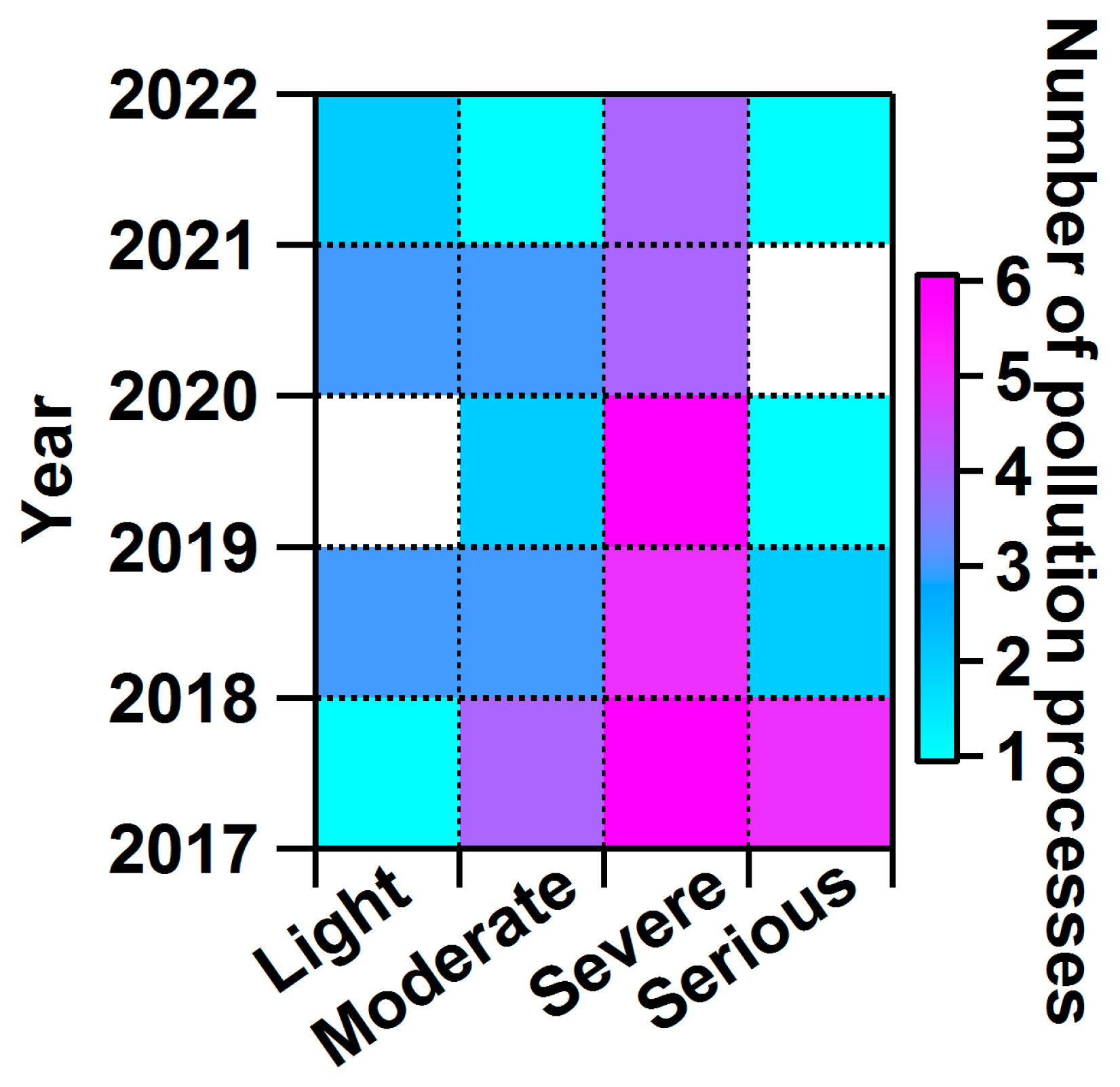
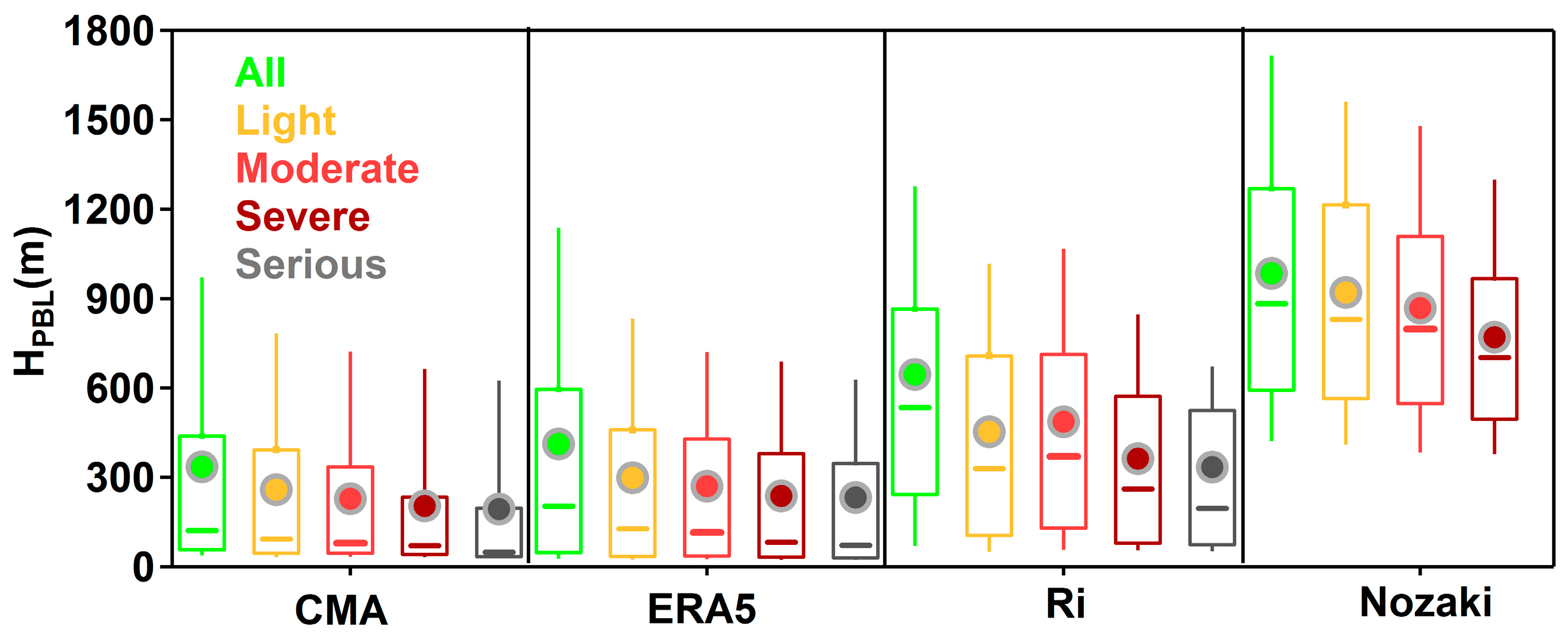
In this paper, L-band radiosonde sounding and surface observation data were used to calculate the BLH in Xi’an for 2017–2021 using the Ri and Nozaki methods, respectively. These results are also used to compare and evaluate the numerical simulation results of CMA and ERA5 in the simultaneous period. For PM_2.5 pollution processes at different levels, the correlation between the vertical structure of meteorological factors and BLH is explored, which can provide the data and theoretical support for development of haze numerical forecasts. The main conclusions are as follows:

1.

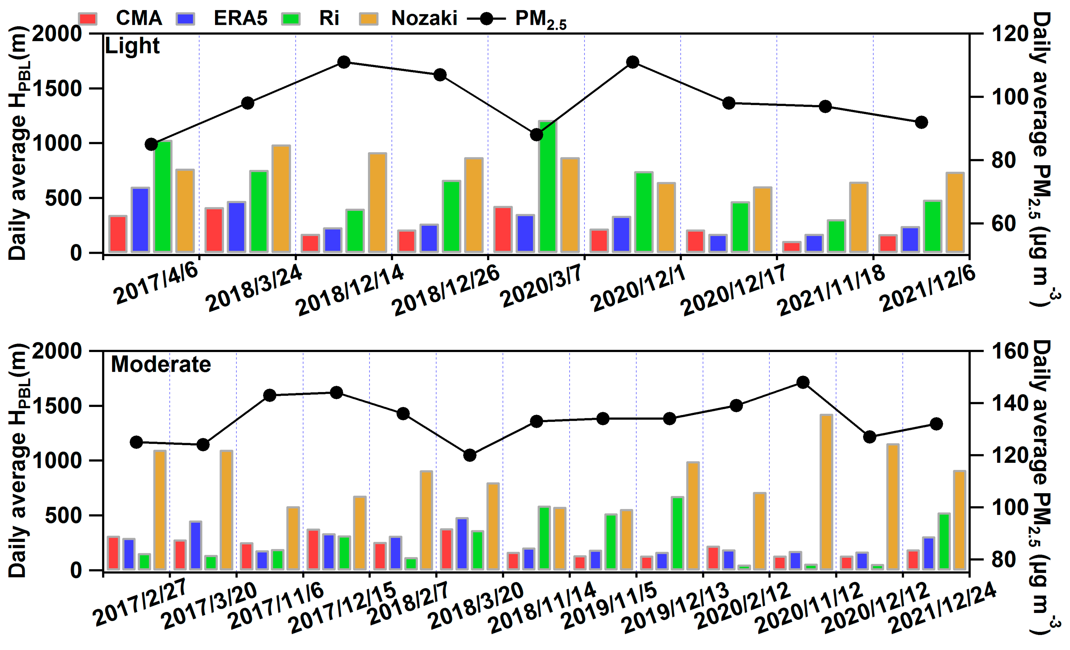
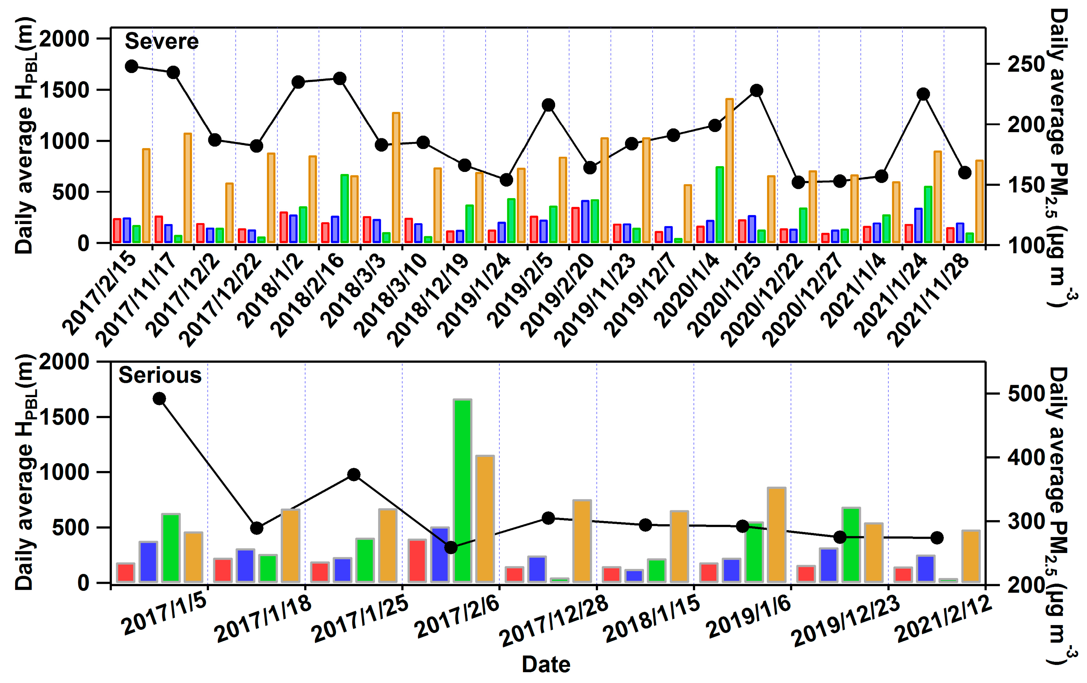
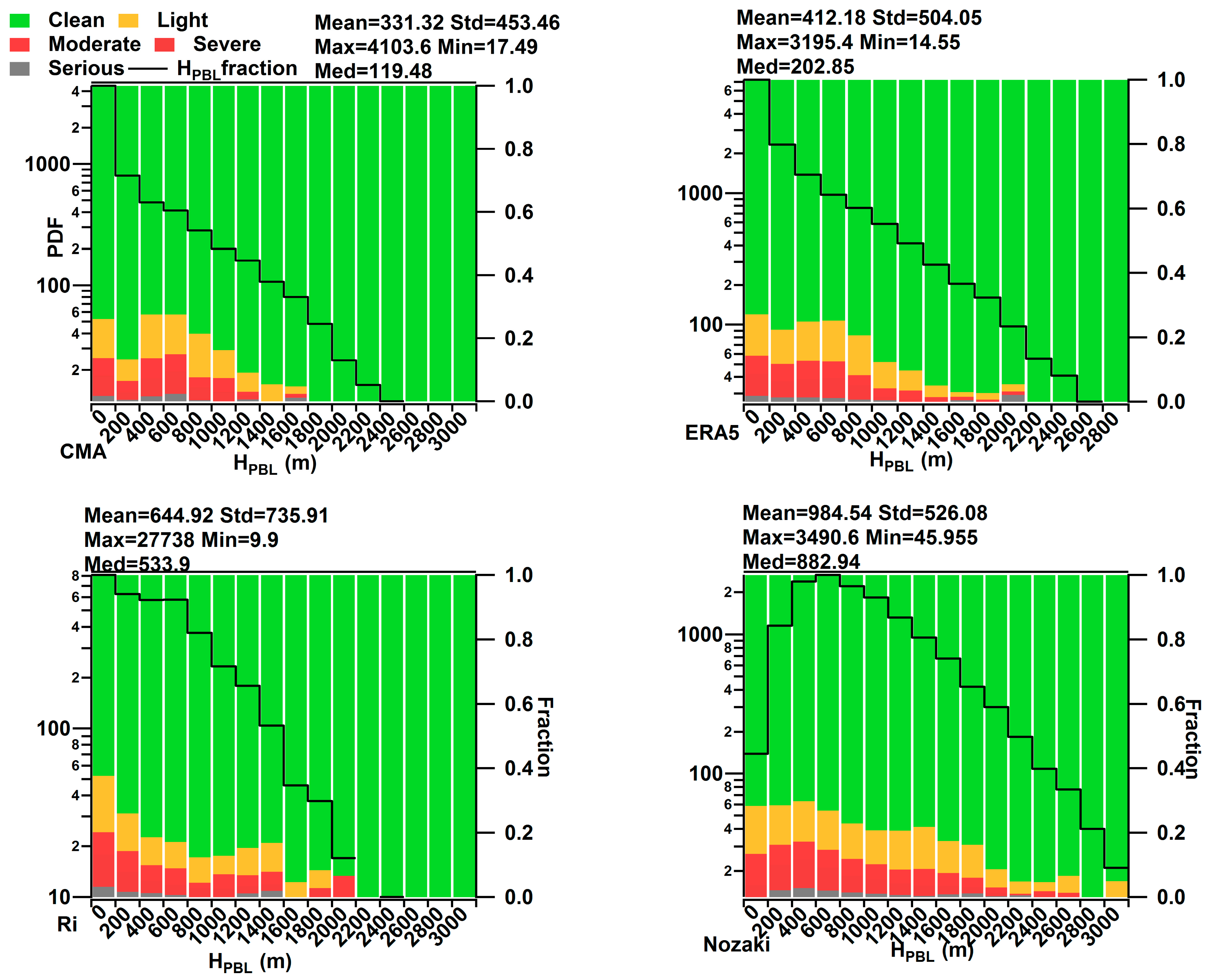
From 2017 to 2021, there was a total of 52 PM_2.5 pollution events in Xi’an, which shows a gradual decreasing trend of moderate, severe and serious pollution and an insignificant trend of light pollution year by year. For the statistical results of all BLH samples, the mean BLH values obtained by Nozaki, Ri, ERA5 and CMA methods from high to low are ~980 m, ~640 m, ~410 m and ~240 m, respectively. The BLH obtained by all four methods decrease gradually with the increase of PM_2.5 pollution level, indicating that there is a certain negative correlation between BLH and PM_2.5 concentration.

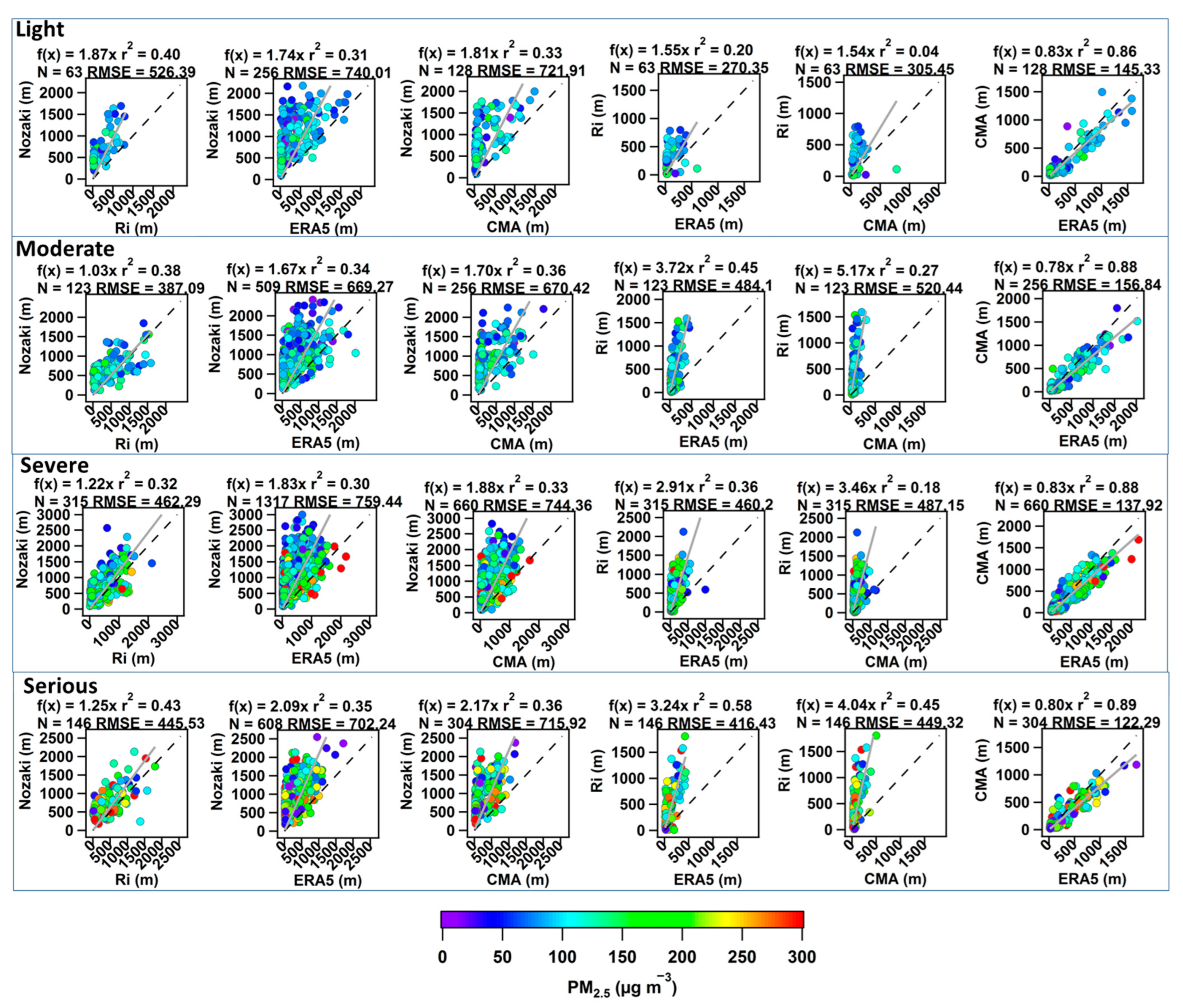
2.

Among the four BLH calculation methods, ERA5-BLH and CMA-BLH have the highest correlation with $r^2$ > 0.85 in all pollution cases, while the correlation between the model and observational method or between Nozaki and Ri methods are significantly lower ($r^2$ < 0.58). The BLH calculated by observation data is generally higher than the model results. The Nozaki method has a good adaptability on the light pollution, and Ri-BLH is more applicable to a stable boundary layer. In moderate or higher pollution, the performance of ERA5-BLH is slightly higher than that of CMA-BLH, and in light pollution there is significant underestimation of both model results. Overall, the correlation among the four BLH methods increases gradually with the increase of pollution level.

3.

In this study, more than 95% cases of the PM_2.5 peak concentration occur on the end day or 1–2 days before the end of the pollution processes with a low BLH; and, there is about ~30% probability of polluted weather with a very low BLH (<200 m) and only <7% probability when BLH > 2000 m.

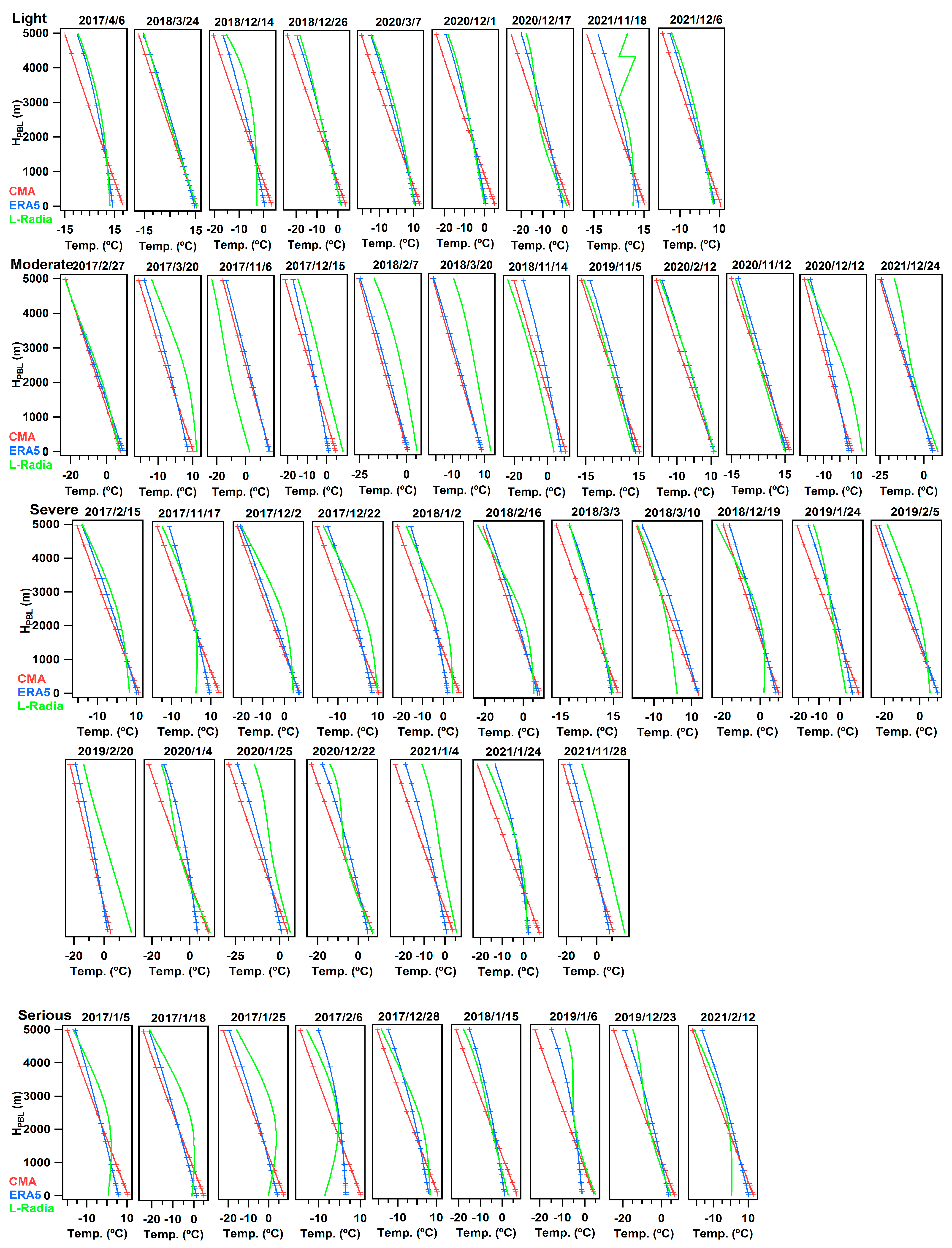
4.

The probability of thermal inversion increases significantly with the increase of pollution level. Compared with the observation results, it is difficult to simulate the neutral boundary layer and inversion processes for CMA and ERA5, especially if there is a large error in the modeling of near-ground temperature. The temperature vertical curve of CMA is closer to that of sounding observations, while ERA5 has higher forecasting skills in boundary layer stability prediction.

The above conclusions, including the relationship between the BLH and the PM_2.5 pollution processes, the underestimation of the simulation BLH of CMA-GFS, and the PM_2.5 forecast inaccuracy of the CUACE, will become the basis and impetus for us to improve the atmospheric boundary layer parameterization scheme of CMA and atmospheric chemistry parameterization scheme of CUACE in the next step.

References

1. Jiang, Q.; Sun, Y.L.; Wang, Z.; Yin, Y. Aerosol composition and sources during the Chinese Spring Festival: Fireworks, secondary aerosol, and holiday effects. Atmos. Chem. Phys. 2015, 15, 6023–6034. [Google Scholar] [CrossRef]
2. Sulaymon, I.D.; Zhang, Y.; Hu, J.; Hopke, P.K.; Zhang, Y.; Zhao, B.; Xing, J.; Li, L.; Mei, X. Evaluation of regional transport of PM2.5 during severe atmospheric pollution episodes in the western Yangtze River Delta, China. J. Environ. Manag. 2021, 293, 112827. [Google Scholar] [CrossRef] [PubMed]
3. Sun, Y.; Lei, L.; Zhou, W.; Chen, C.; He, Y.; Sun, J.; Li, Z.; Xu, W.; Wang, Q.; Ji, D.; et al. A chemical cocktail during the COVID-19 outbreak in Beijing, China: Insights from six-year aerosol particle composition measurements during the Chinese New Year holiday. Sci. Total Environ. 2020, 742, 140739. [Google Scholar] [CrossRef] [PubMed]
4. Dang, R.; Liao, H. Severe winter haze days in the Beijing–Tianjin–Hebei region from 1985 to 2017 and the roles of anthropogenic emissions and meteorology. Atmos. Chem. Phys. 2019, 19, 10801–10816. [Google Scholar] [CrossRef]
5. Zhang, X.; Xu, X.; Ding, Y.; Liu, Y.; Zhang, H.; Wang, Y.; Zhong, J. The impact of meteorological changes from 2013 to 2017 on PM2.5 mass reduction in key regions in China. Sci. China Earth Sci. 2019, 62, 1885–1902. [Google Scholar] [CrossRef]
6. Zhang, R.; Rui, S.; Wang, W.; Wang, J.; Hao, Y. Effects of meteorological conditions on the characteristics of near-surface atmospheric environmental pollution in summer and winter in Xi’an, China. Ecol. Environ. Sci. 2020, 29, 165–174. (In Chinese) [Google Scholar]
7. Yim, S.H.L. Development of a 3D Real-Time Atmospheric Monitoring System (3DREAMS) Using Doppler LiDARs and Applications for Long-Term Analysis and Hot-and-Polluted Episodes. Remote Sens. 2020, 12, 1036. [Google Scholar] [CrossRef]
8. Liu, B.; Ma, Y.; Gong, W.; Zhang, M.; Yang, J. Determination of boundary layer top on the basis of the characteristics of atmospheric particles. Atmos. Environ. 2018, 178, 140–147. [Google Scholar] [CrossRef]
9. Miao, S.; Chen, F.; Li, Q.; Fan, S. Impacts of Urban Processes and Urbanization on Summer Precipitation: A Case Study of Heavy Rainfall in Beijing on 1 August 2006. J. Appl. Meteorol. Clim. 2011, 50, 806–825. [Google Scholar] [CrossRef]
10. Wang, L.; Wang, H.; Liu, J.; Gao, Z.; Yang, Y.; Zhang, X.; Li, Y.; Huang, M. Impacts of the near-surface urban boundary layer structure on PM2.5 concentrations in Beijing during winter. Sci. Total Environ. 2019, 669, 493–504. [Google Scholar] [CrossRef]
11. Liu, Q.; Jia, X.; Quan, J.; Li, J.; Li, X.; Wu, Y.; Chen, D.; Wang, Z.; Liu, Y. New positive feedback mechanism between boundary layer meteorology and secondary aerosol formation during severe haze events. Sci. Rep. 2018, 8, 6095. [Google Scholar] [CrossRef]
12. Lolli, S.; Khor, W.Y.; Matjafri, M.Z.; Lim, H.S. Monsoon Season Quantitative Assessment of Biomass Burning Clear-Sky Aerosol Radiative Effect at Surface by Ground-Based Lidar Observations in Pulau Pinang, Malaysia in 2014. Remote Sens. 2019, 11, 2660. [Google Scholar] [CrossRef]
13. Zhong, J.; Zhang, X.; Wang, Y. Reflections on the threshold for PM2.5 explosive growth in the cumulative stage of winter heavy aerosol pollution episodes (HPEs) in Beijing. Tellus B Chem. Phys. Meteorol. 2019, 71, 1528134. [Google Scholar] [CrossRef]
14. Shi, Y.; Hu, F.; Fan, G.; Zhang, Z. Multiple technical observations of the atmospheric boundary layer structure of a red-alert haze episode in Beijing. Atmos. Meas. Tech. 2019, 12, 4887–4901. [Google Scholar] [CrossRef]
15. Zhong, J.; Zhang, X.; Dong, Y.; Wang, Y.; Liu, C.; Wang, J.; Zhang, Y.; Che, H. Feedback effects of boundary-layer meteorological factors on cumulative explosive growth of PM2.5 during winter heavy pollution episodes in Beijing from 2013 to 2016. Atmos. Meas. Tech. 2018, 18, 247–258. [Google Scholar] [CrossRef]
16. Zhang, H.; Zhang, X.; Li, Q.; Cai, X.; Fan, S.; Song, Y.; Hu, F.; Che, H.; Quan, J.; Kang, L.; et al. Research progress on estimation of atmospheric boundary layer height. Acta Meteorol. Sin. 2020, 78, 522–536. (In Chinese) [Google Scholar] [CrossRef]
17. Quan, J.; Gao, Y.; Zhang, Q.; Tie, X.; Cao, J.; Han, S.; Meng, J.; Chen, P.; Zhao, D. Evolution of planetary boundary layer under different weather conditions, and its impact on aerosol concentrations. Particuology 2012, 11, 34–40. [Google Scholar] [CrossRef]
18. Seibert, P.; Beyrich, F.; Gryning, S.-E.; Joffre, S.; Rasmussen, A.; Tercier, P. Review and intercomparison of operational methods for the determination of the mixing height. Atmos. Environ. 2000, 34, 1001–1027. [Google Scholar] [CrossRef]
19. Miao, Y.; Liu, S. Linkages between aerosol pollution and planetary boundary layer structure in China. Sci. Total Environ. 2018, 650, 288–296. [Google Scholar] [CrossRef]
20. Miao, Y.; Guo, J.; Liu, S.; Zhao, C.; Li, X.; Zhang, G.; Wei, W.; Ma, Y. Impacts of synoptic condition and planetary boundary layer structure on the trans-boundary aerosol transport from Beijing-Tianjin-Hebei region to northeast China. Atmos. Environ. 2018, 181, 1–11. [Google Scholar] [CrossRef]
21. Wei, J.; Tang, G.; Zhu, X.; Wang, L.; Liu, Z.; Cheng, M.; Münkel, C.; Li, X.; Wang, Y. Thermal internal boundary layer and its effects on air pollutants during summer in a coastal city in North China. J. Environ. Sci. 2017, 70, 37–44. [Google Scholar] [CrossRef] [PubMed]
22. Ye, X.; Song, Y.; Cai, X.; Zhang, H. Study on the synoptic flow patterns and boundary layer process of the severe haze events over the North China Plain in January 2013. Atmos. Environ. 2016, 124, 129–145. [Google Scholar] [CrossRef]
23. Leng, C.; Duan, J.; Xu, C.; Zhang, H.; Zhang, Q.; Wang, Y.; Li, X.; Kong, L.; Tao, J.; Cheng, T.; et al. Insights into a historic severe haze weather in Shanghai: Synoptic situation, boundary layer and pollu-tants. Atmos. Chem. Phys. Discuss. 2015, 15, 32561–32605. [Google Scholar] [CrossRef]
24. Xu, J.; Wang, Z.; Yu, G.; Sun, W.; Qin, X.; Ren, J.; Qin, D. Seasonal and diurnal variations in aerosol concentrations at a high-altitude site on the northern boundary of Qinghai-Xizang Plateau. Atmos. Res. 2013, 120–121, 240–248. [Google Scholar] [CrossRef]
25. Fan, S.J.; Fan, Q.; Yu, W.; Luo, X.Y.; Wang, B.M.; Song, L.L.; Leong, K.L. Atmospheric boundary layer characteristics over the Pearl River Delta, China, during the summer of 2006: Measurement and model results. Atmos. Chem. Phys. 2011, 11, 6297–6310. [Google Scholar] [CrossRef]
26. Song, L.; Deng, T.; Wu, D.; He, G.; Sun, J.; Weng, J.; Wu, C. Study on planetary boundary layer height in a typical haze period and different weather types over Guangzhou. Acta Sci. Circumstantiae 2019, 39, 1381–1391. (In Chinese) [Google Scholar] [CrossRef]
27. Li, Q.; Wu, B.; Liu, J.; Zhang, H.; Cai, X.; Song, Y. Characteristics of the atmospheric boundary layer and its relation with PM2.5 during haze episodes in winter in the North China Plain. Atmos. Environ. 2020, 223, 117265. [Google Scholar] [CrossRef]
28. Zhao, H.; Che, H.; Xia, X.; Wang, Y.; Wang, H.; Wang, P.; Ma, Y.; Yang, H.; Liu, Y.; Wang, Y.; et al. Climatology of mixing layer height in China based on multi-year meteorological data from 2000 to 2013. Atmos. Environ. 2019, 213, 90–103. [Google Scholar] [CrossRef]
29. Qu, Y.; Han, Y.; Wu, Y.; Gao, P.; Wang, T. Study of PBLH and Its Correlation with Particulate Matter from One-Year Observation over Nanjing, Southeast China. Remote Sens. 2017, 9, 668. [Google Scholar] [CrossRef]
30. Wang, Q.; Sun, Y.; Xu, W.; Du, W.; Zhou, L.; Tang, G.; Chen, C.; Cheng, X.; Zhao, X.; Ji, D.; et al. Vertically-resolved Char-acteristics of Air Pollution during Two Severe Winter Haze Episodes in Urban Beijing, China. Atmos. Chem. Phys. 2018, 18, 2495–2509. [Google Scholar] [CrossRef]
31. Gui, K.; Che, H.; Wang, Y.; Wang, H.; Zhang, L.; Zhao, H.; Zheng, Y.; Sun, T.; Zhang, X. Satellite-derived PM2.5 concentration trends over Eastern China from 1998 to 2016: Relationships to emissions and meteorological parameters. Environ. Pollut. 2019, 247, 1125–1133. [Google Scholar] [CrossRef]
32. Ma, M.; Pu, Z.; Wang, S.; Zhang, Q. Characteristics and Numerical Simulations of Extremely Large Atmospheric Boundary-layer Heights over an Arid Region in North-west China. Bound.-Layer Meteorol. 2011, 140, 163–176. [Google Scholar] [CrossRef]
33. Seidel, D.J.; Zhang, Y.; Beljaars, A.; Golaz, J.-C.; Jacobson, A.R.; Medeiros, B. Climatology of the planetary boundary layer over the continental United States and Europe. J. Geophys. Res. Atoms. 2012, 117. [Google Scholar] [CrossRef]
34. Liu, S.; Liang, X.-Z. Observed Diurnal Cycle Climatology of Planetary Boundary Layer Height. J. Clim. 2010, 23, 5790–5809. [Google Scholar] [CrossRef]
35. Vickers, D.; Mahrt, L. Evaluating formulations of stable boundary layer height. J. Appl. Meteor. 2004, 43, 1736–1749. [Google Scholar] [CrossRef]
36. Nozaki, K.Y. Mixing Depth Model Using Hourly Surface Observations; Report 7053; USAF Environmental Technical Application Center: Scott AFB, IL, USA, 1973. [Google Scholar]
37. Liu, C.; Hua, C.; Zhang, H.; Lv, M.; Zhang, B. Application of L-band radar sounding datain analyziing polluted weather boundary layer. Meteorol. Mon. 2017, 043, 591–597. (In Chinese) [Google Scholar] [CrossRef]
38. Li, H.; Liu, B.; Ma, X.; Jin, S.; Ma, Y.; Zhao, Y.; Gong, W. Evaluation of retrieval methods for planetary boundary layer height based on radiosonde data. Atmos. Meas. Tech. 2021, 14, 5977–5986. [Google Scholar] [CrossRef]
39. Banks, R.F.; Tiana-Alsina, J.; Baldasano, J.M.; Rocadenbosch, F.; Papayannis, A.; Solomos, S.; Tzanis, C.G. Sensitivity of boundary-layer variables to PBL schemes in the WRF model based on surface meteorological observations, lidar, and radiosondes during the HygrA-CD campaign. Atmos. Res. 2016, 176–177, 185–201. [Google Scholar] [CrossRef]
40. Li, T.; Wang, H.; Zhao, T.; Xue, M.; Wang, Y.; Che, H.; Jiang, C. The Impacts of Different PBL Schemes on the Simulation of PM2.5 during Severe Haze Episodes in the Jing-Jin-Ji Region and Its Surroundings in China. Adv. Meteorol. 2016, 2016, 6295878. [Google Scholar] [CrossRef]
41. Musthafa, M.; Turyanti, A.; Nuryanto, D.E. Sensitivity of Planetary Boundary Layer Scheme in WRF-Chem Model for Predicting PM10 Concentration (Case study: Jakarta). IOP Conf. Ser. Earth Environ. Sci. 2019, 303, 012049. [Google Scholar] [CrossRef]
42. Zhu, W.; Li, H.W.; Wang, B.M.; Wu, M.; Bu, Q.L.; Dong, G.Y.; Yan, L.J.; Fan, S.J. Joint application of multiple remote sensing equipment on the study of the relationship between regional air quality change and boundary layer structure. Acta Sci. Circumstantiae 2018, 38, 1689–1698. (In Chinese) [Google Scholar] [CrossRef]
43. Chen, J.; Ma, Z.; Li, Z.; Shen, X.; Su, Y.; Chen, Q.; Liu, Y. Vertical diffusion and cloud scheme coupling to the Charney–Phillips vertical grid in GRAPES global forecast system. Q. J. R. Meteorol. Soc. 2020, 146, 2191–2204. [Google Scholar] [CrossRef]
44. Long, H.; Chen, Q.; Gong, X.; Zhu, K. Evaluation of the Planetary Boundary Layer Height in China Predicted by the CMA-GFS Global Model. Atmosphere 2022, 13, 845. [Google Scholar] [CrossRef]
45. Mason, P. Boundary-layer parametrization in heterogeneous terrain. In Proceedings of the Workshop on Fine-Scale Modelling and the Development of Parametrization Schemes, Berkshire, UK, 16–18 September 1991. [Google Scholar]
46. Vogelezang, D.H.P.; Holtslag, B. Evaluation and model impacts of alternative boundary-layer height formulations. Bound.-Layer Meteorol. 1996, 81, 245–269. [Google Scholar] [CrossRef]
47. Du, C.; Liu, S.; Yu, X.; Li, X.; Chen, C.; Peng, Y.; Dong, Y.; Dong, Z.; Wang, F. Urban Boundary Layer Height Characteristics and Relationship with Particulate Matter Mass Concentrations in Xi’an, Central China. Aerosol Air Qual. Res. 2013, 13, 1598–1607. [Google Scholar] [CrossRef]
48. Ma, J.; Zheng, X. Comparisons of Boundary Mixing Layer Heights at 7 Sites in China: Radiosonde Measurement Determination and the Empirical Calculation. J. Appl. Meteorol. Sci. 2011, 22, 567–576. (In Chinese) [Google Scholar]
49. GB 3092-2012; Technical Regulation of National Standard System on Ambient Air Quality Standards. Available online: https://www.mee.gov.cn/ywgz/fgbz/bz/bzwb/dqhjbh/dqhjzlbz/201203/W020120410330232398521.pdf (accessed on 29 February 2012).
50. Guo, J.; Zhang, J.; Yang, K.; Liao, H.; Zhang, S.; Huang, K.; Lv, Y.; Shao, J.; Yu, T.; Tong, B.; et al. Investigation of near-global daytime boundary layer height using high-resolution radiosondes: First results and comparison with ERA5, MERRA-2, JRA-55, and NCEP-2 reanalyses. Atmos. Chem. Phys. 2021, 21, 17079–17097. [Google Scholar] [CrossRef]
51. Dong, Z.; Li, Z.; Yu, X.; Cribb, M.; Li, X.; Dai, J. Opposite Long-term Trends in Aerosols between Lower and Higher Altitudes: A Testimony to the Aerosol-PBL Feedback. Atmos. Chem. Phys. 2017, 17, 7997–8009. [Google Scholar] [CrossRef]
52. Li, L.; Lu, C.; Chan, P.-W.; Zhang, X.; Yang, H.-L.; Lan, Z.-J.; Zhang, W.-H.; Liu, Y.-W.; Pan, L.; Zhang, L. Tower observed vertical distribution of PM2.5, O3 and NOx in the Pearl River Delta. Atmos. Environ. 2019, 220, 117083. [Google Scholar] [CrossRef]
53. Largeron, Y.; Staquet, C. Persistent inversion dynamics and wintertime PM10 air pollution in Alpine valleys. Atmos. Environ. 2016, 135, 92–108. [Google Scholar] [CrossRef]
54. Gong, S.L.; Barrie, L.A.; Blanchet, J.; Von Salzen, K.; Lohmann, U.; Lesins, G.; Špaček, L.; Zhang, L.M.; Girard, E.; Lin, H.; et al. Canadian Aerosol Module: A size-segregated simulation of atmospheric aerosol processes for climate and air quality models 1. Module development. J. Geophys. Res. Atmos. 2003, 108, 4007. [Google Scholar] [CrossRef]
Figure 1. Geographic location of Xi’an (a) and air quality forecast range (b), where the red point is the location of the Jinghe station in Xi’an, and the blue point is the location of the PM2.5 monitoring station.
Atmosphere 14 00728 g001
Figure 2. Annual evolution of the number of different PM2.5 pollution level processes from 2017 to 2021.
Atmosphere 14 00728 g002
Figure 3. Statistics of the results of the four BLH methods for all and different levels of PM2.5 pollution processes from 2017 to 2021. (HPBL: BLH; all: 52 PM2.5 pollution processes; Light: light pollution processes; Moderate: moderate pollution processes; Severe: severe pollution processes; Serious: serious pollution processes; solid circle are mean values, short horizontal lines from top to bottom are 75th, median and 25th quartiles respectively, vertical lines indicate 90th and 10th quartiles).
Atmosphere 14 00728 g003
Figure 4. BLH scatter diagram of four BLH methods under different pollution processes. ( r 2 : correlation coefficient; N: number of samples; RMSE: Root-mean-square Error; Color indicates the mass concentration of PM2.5).
Atmosphere 14 00728 g004
Figure 5. The histogram of different BLH values and the diagram of PM2.5 concentrations in peak concentration days under different pollution processes. (CMA−BLH: red bar; ERA5-BLH: blue bar; Ri-BLH: geen bar; Nozaki−BLH: goldenrod bar; PM2.5 concentration: dotted line).
Atmosphere 14 00728 g005aAtmosphere 14 00728 g005b
Figure 6. The probability distribution diagram of BLH and the proportion of different levels of PM2.5 pollution from the four BLH calculation methods. (The left vertical axis is BLH, the right vertical axis is the probability distribution for different levels of PM2.5 pollution; black short line is the number of occurrences of BLH in different interval, corresponding to the left logarithmic co-ordinates; the color bars are the proportion of different levels of PM2.5 pollution, corresponding to the right coordinates; the upper right or left corner of each panel shows the statistical parameter of BLH).
Atmosphere 14 00728 g006
Figure 7. The vertical profiles of CMA, ERA5 and L−band radiosonde sounding temperature in peak concentration days under different levels of PM2.5 pollution processes.
Atmosphere 14 00728 g007
Figure 8. The PM2.5 concentration distribution of 25 January 2017 and 6 December 2021 cases simulated by CMA−CUACE (the soild dots represent the observed values).
Atmosphere 14 00728 g008
Disclaimer/Publisher’s Note: The statements, opinions and data contained in all publications are solely those of the individual author(s) and contributor(s) and not of MDPI and/or the editor(s). MDPI and/or the editor(s) disclaim responsibility for any injury to people or property resulting from any ideas, methods, instructions or products referred to in the content.