
Assessing Urban Flood Hazard Vulnerability Using Multi-Criteria Decision Making and Geospatial Techniques in Nabadwip Municipality, West Bengal in India
 ,
,  , ,
, ,
Abstract
:1. Introduction
- To identify the physical and environmental factors of flood hazard in the study area in 2000 and 2015;
- To delineate the flood vulnerability zones in the study area in 2000 and 2015;
- To analyze the relationship between flood vulnerability and urban development;
- To measure a flood mitigation strategy using strengths–weaknesses–opportunities–challenges analysis.
2. Hypothesis
3. Materials and Methods
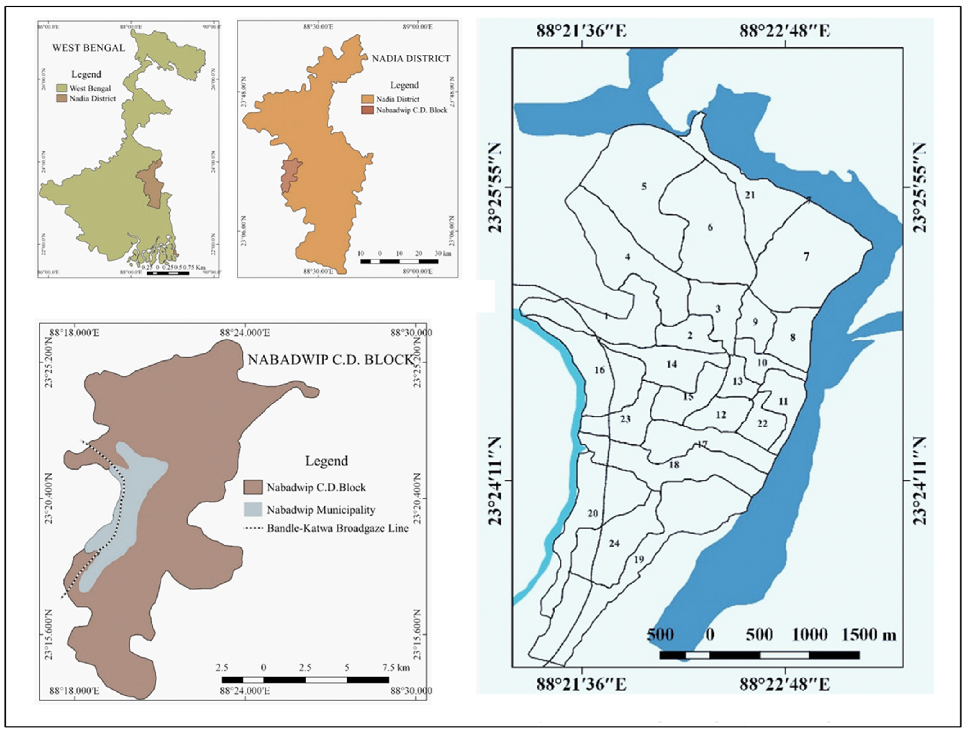
3.1. Study Area
3.2. Data Sources
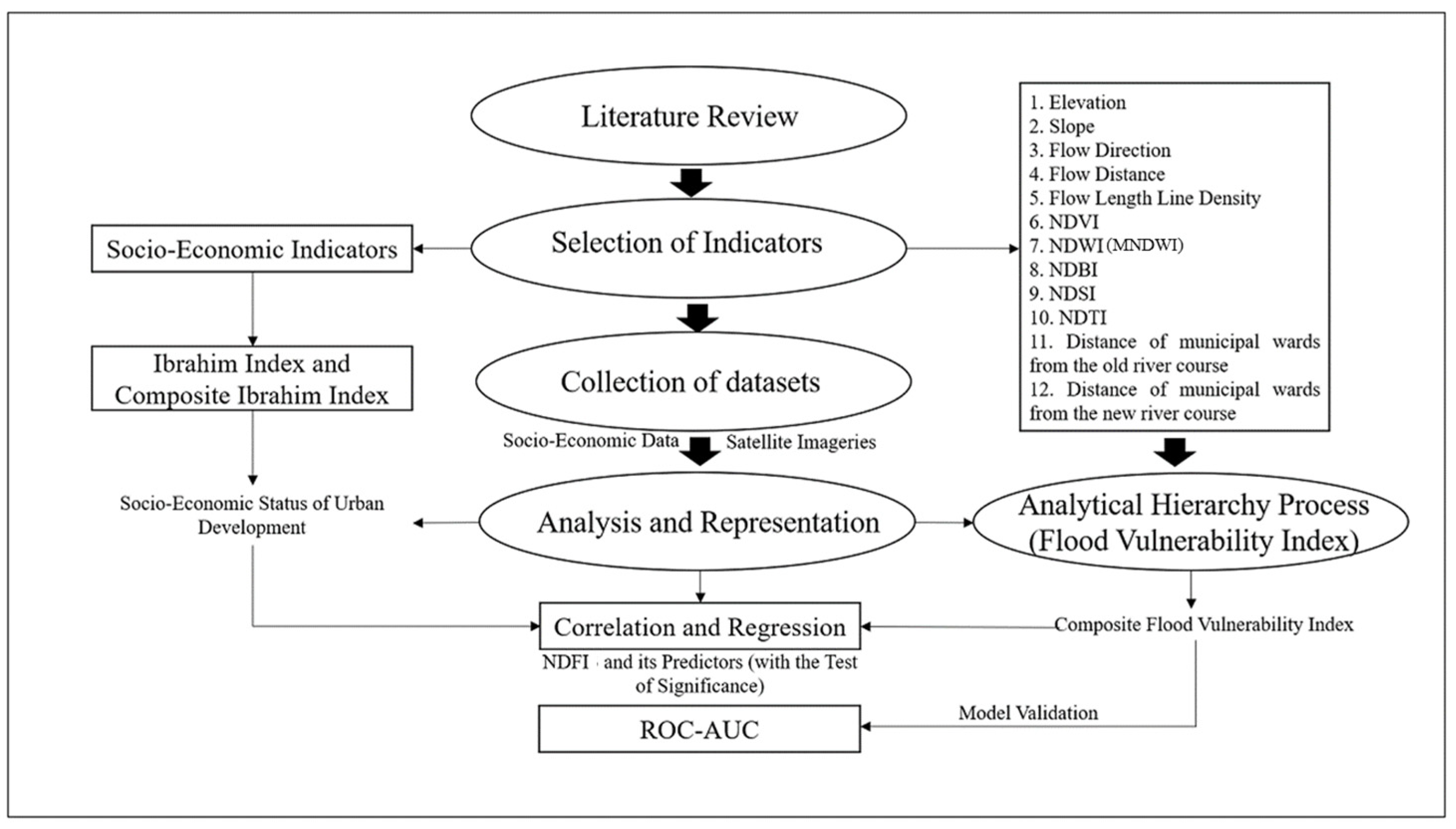
3.3. Research Design
3.4. Methods and Techniques
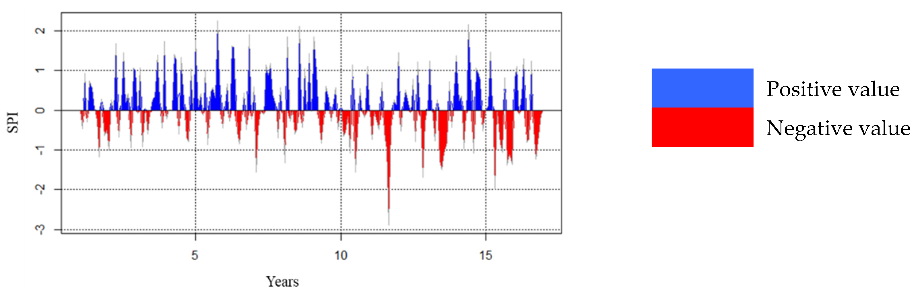
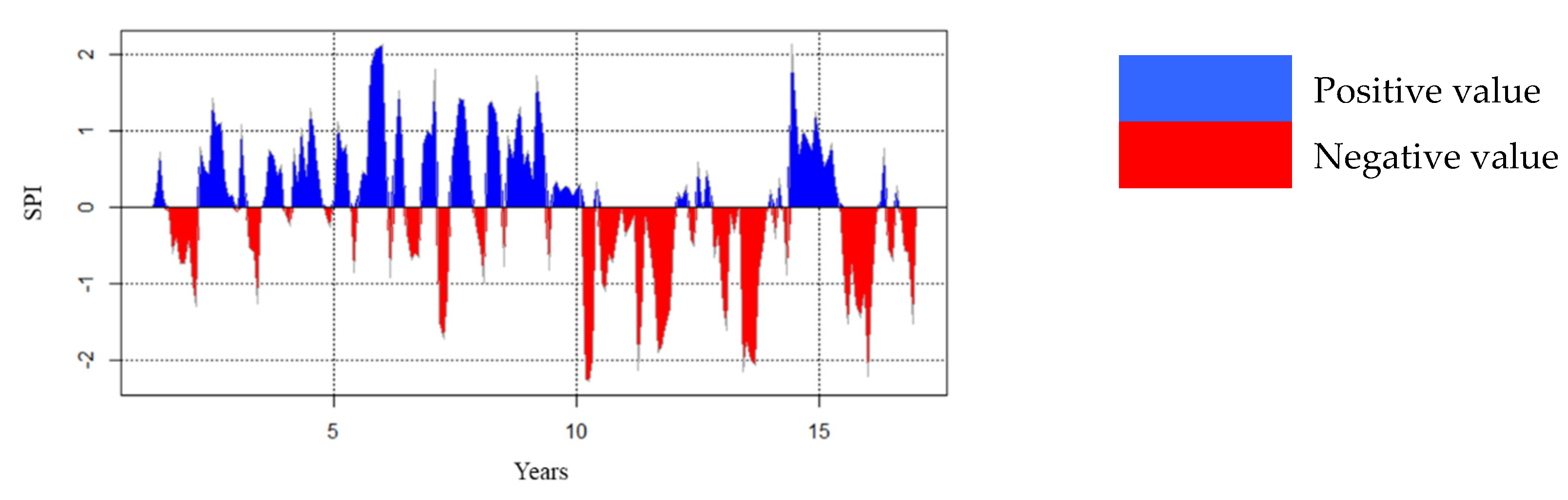
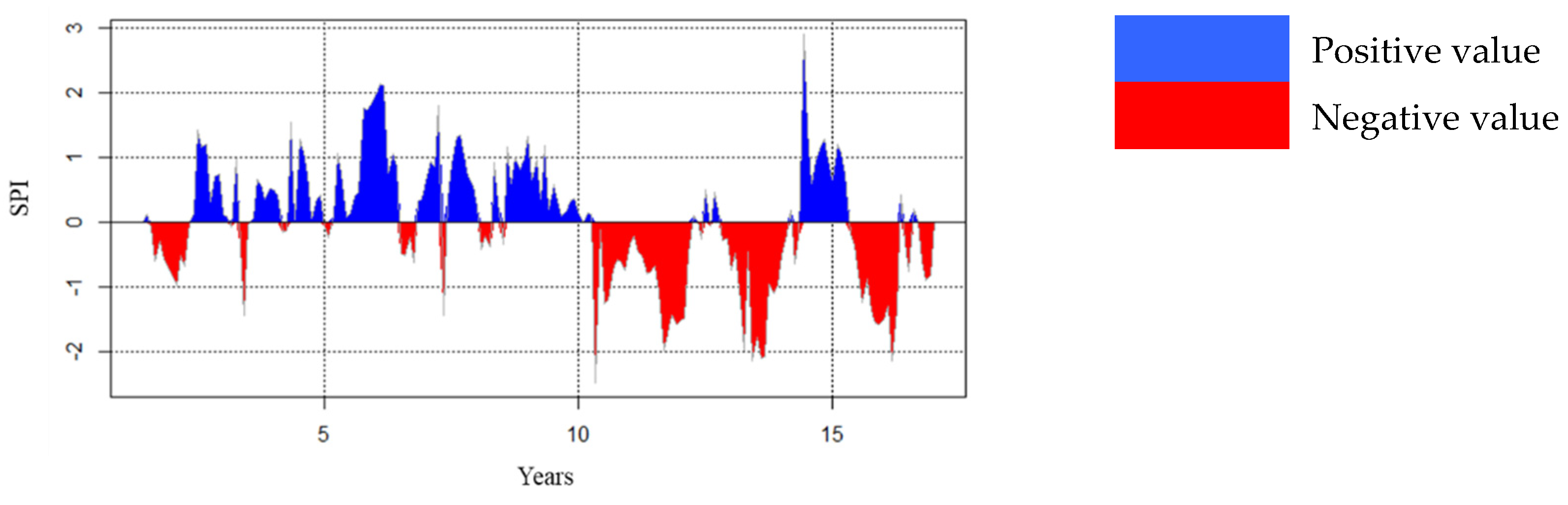
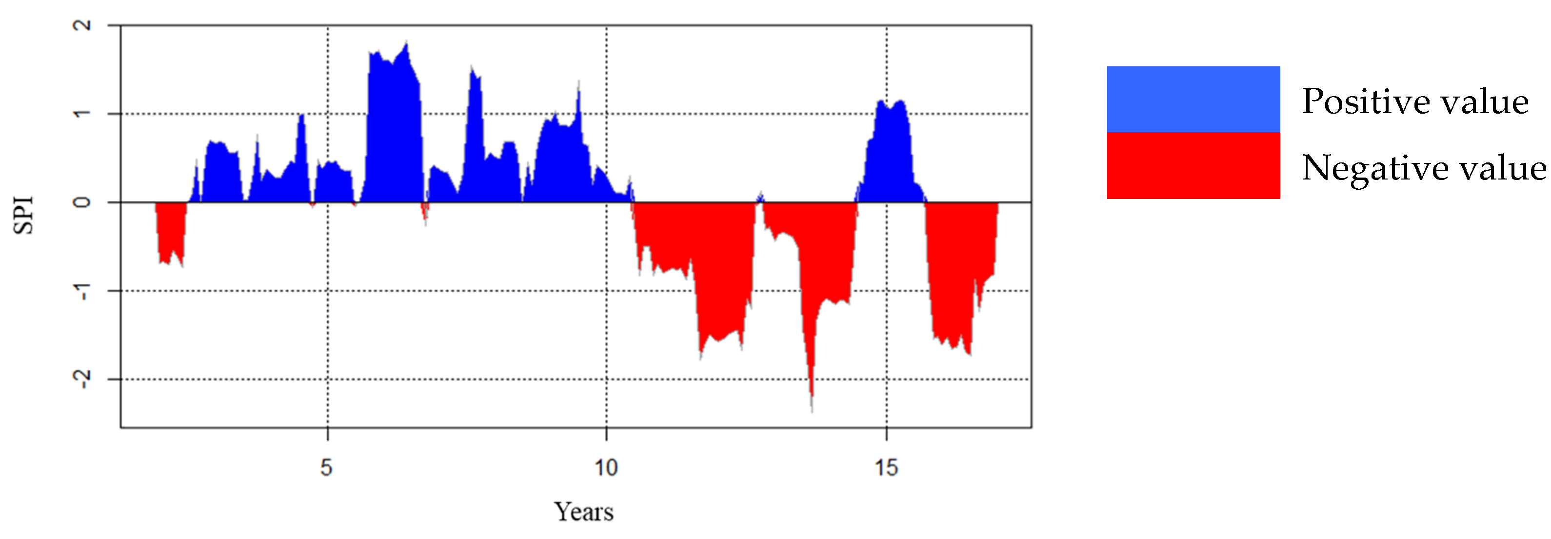
3.4.1. Standardized Precipitation Index (SPI) Analysis
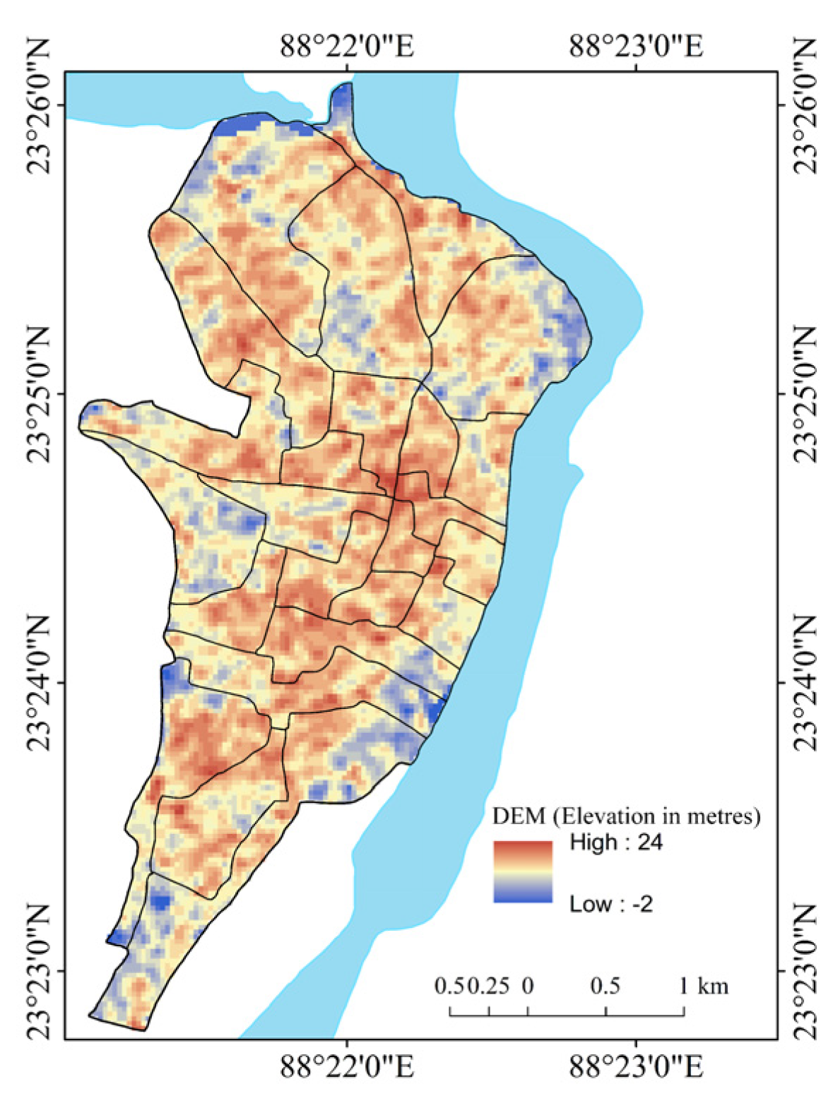
3.4.2. Digital Elevation Model (DEM) and Raster Analyses
3.4.3. Flood Vulnerability Index (FVI)
3.4.4. Composite Ibrahim Index (CIb) of Socio-Economic Development
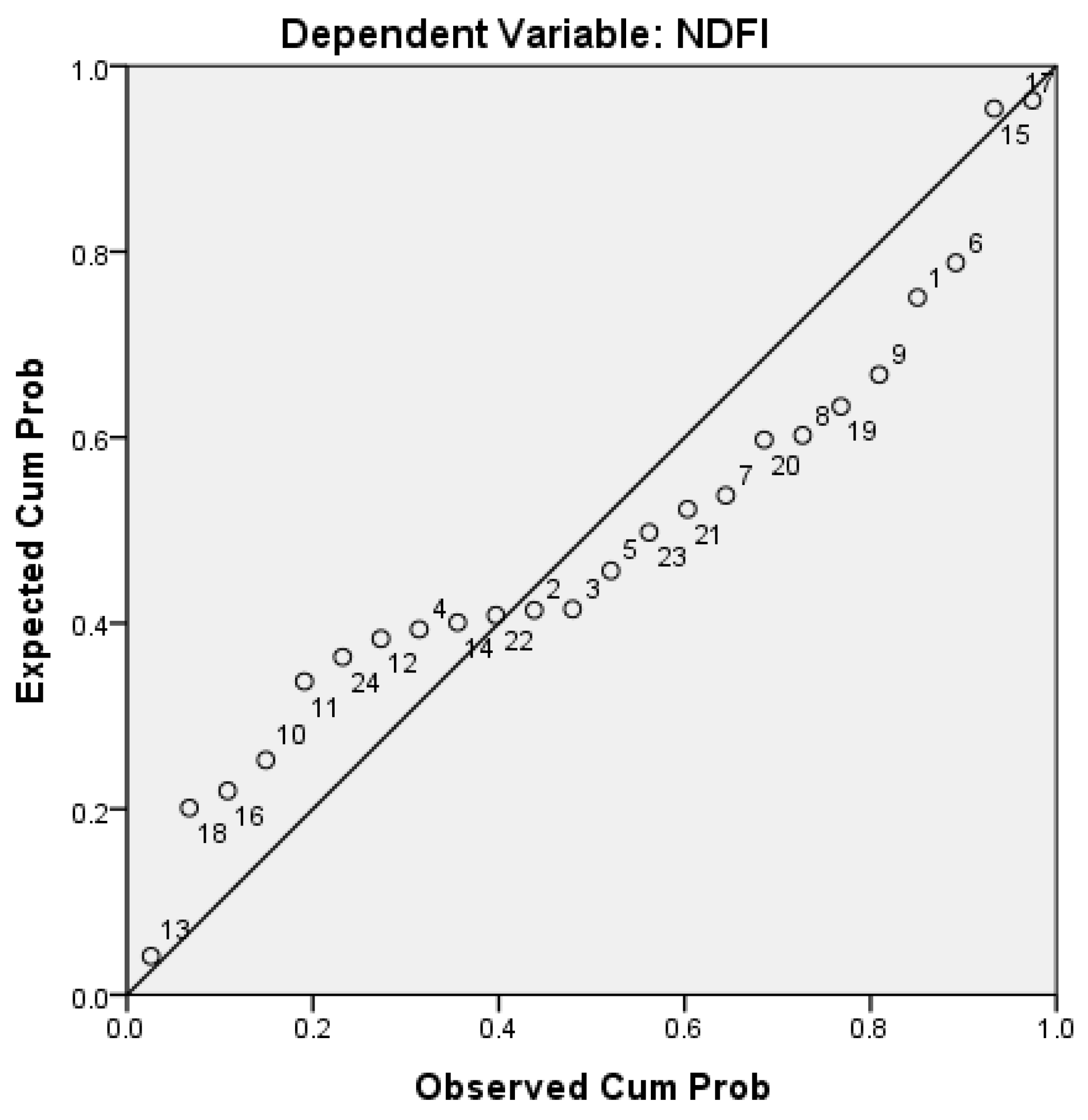
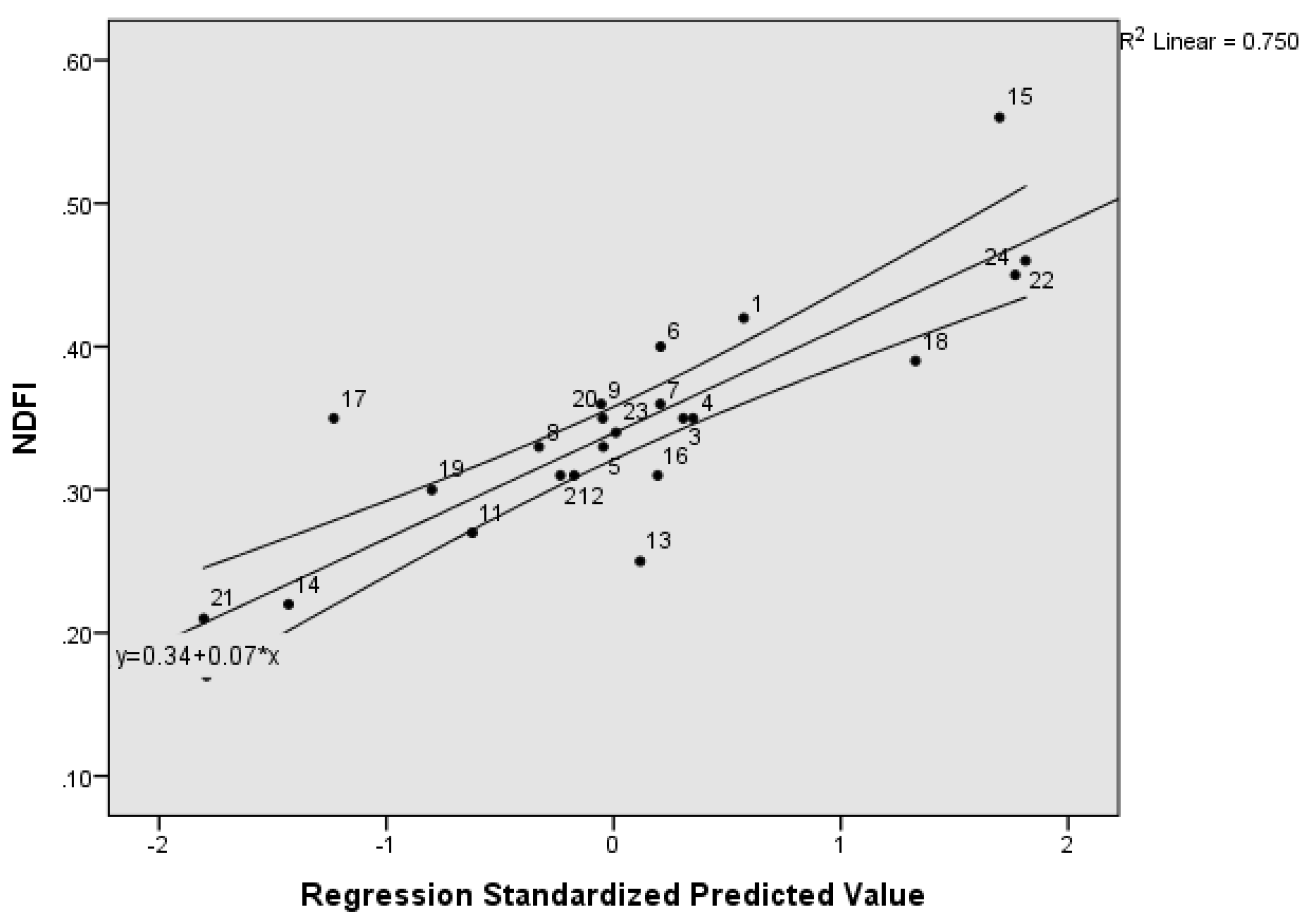
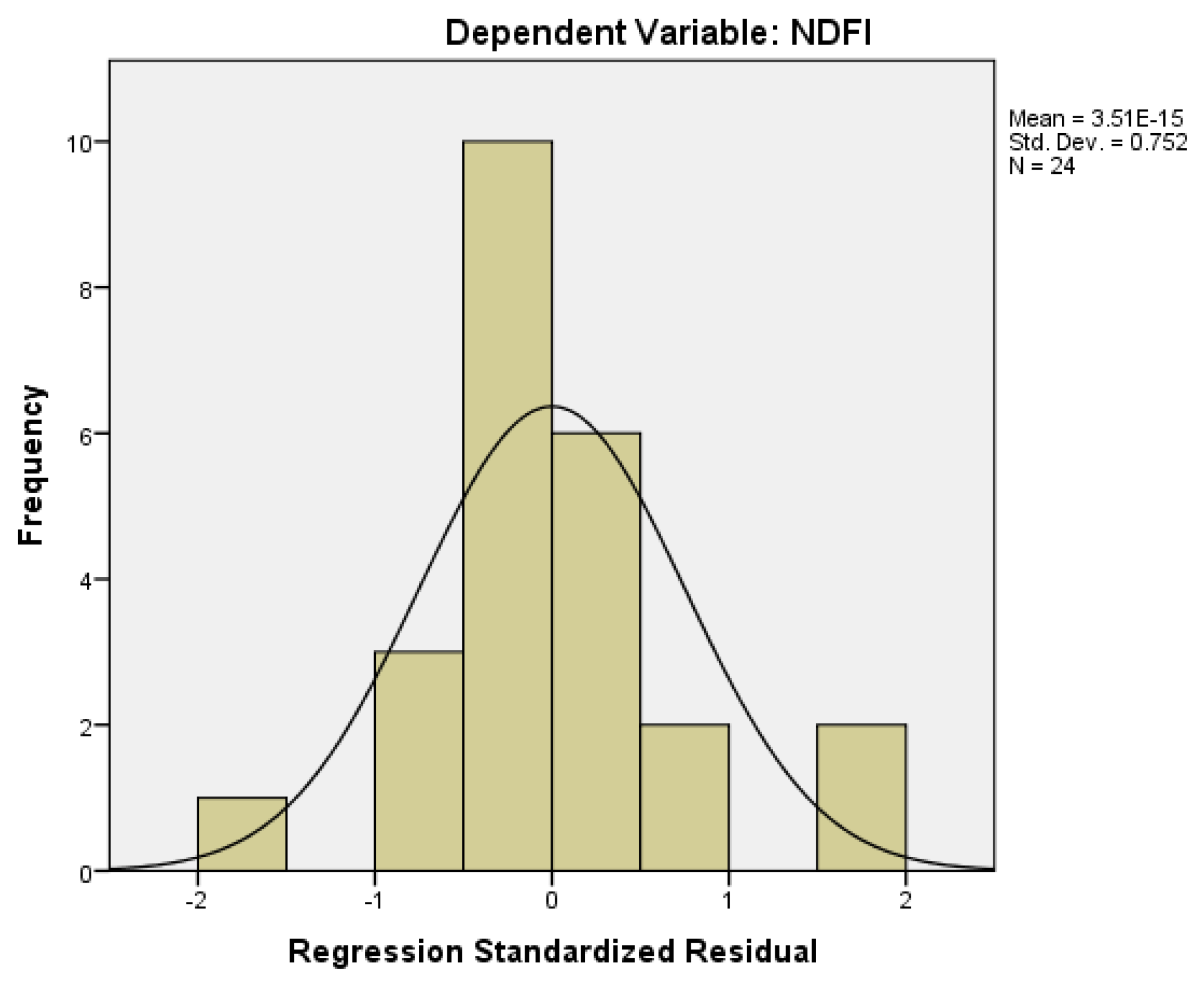
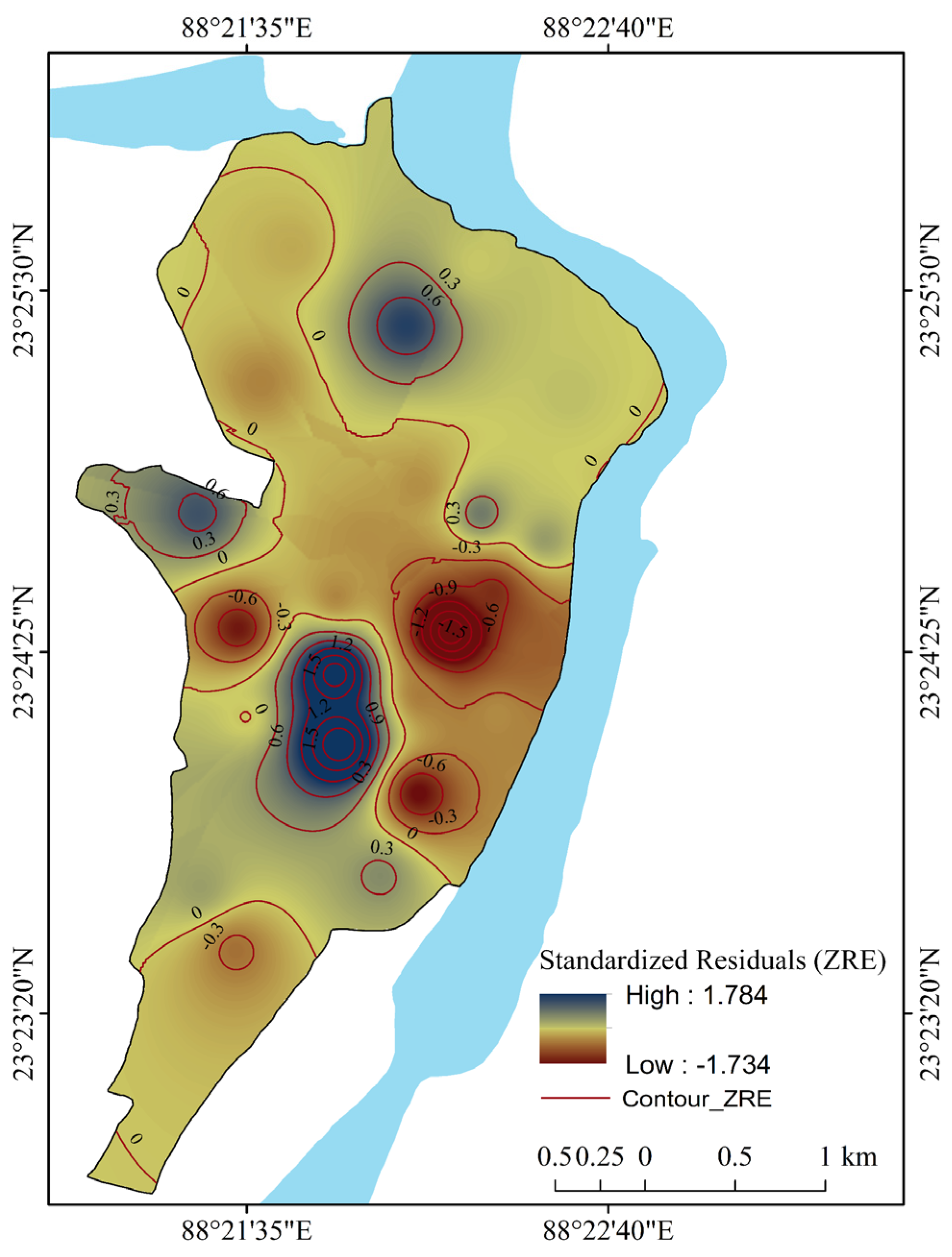
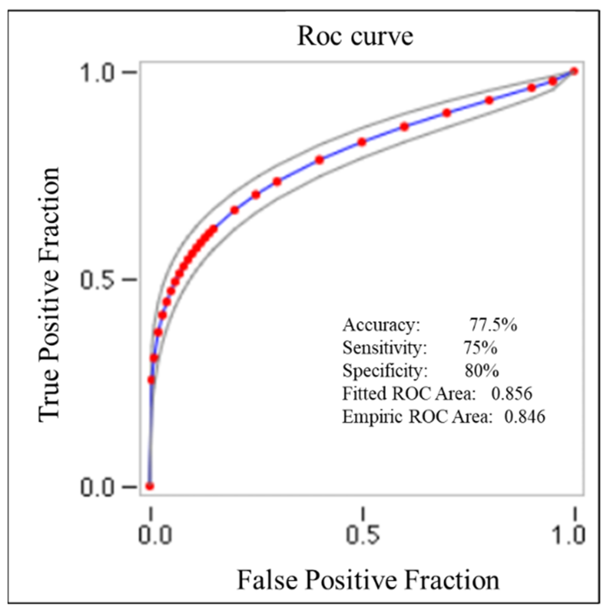
3.4.5. Correlation, Regression, Hypothesis Testing, and Model Validation
4. Results
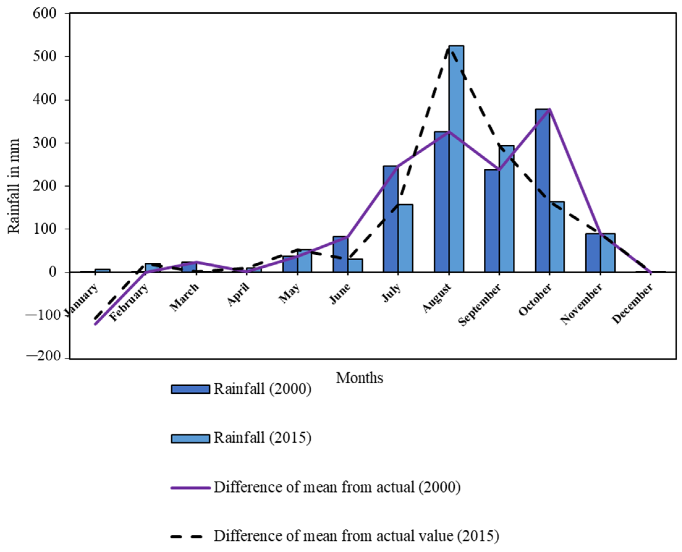
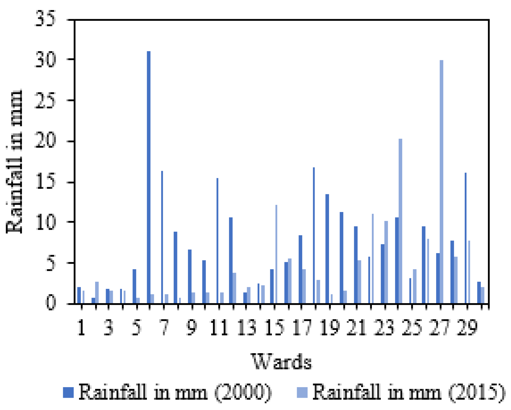
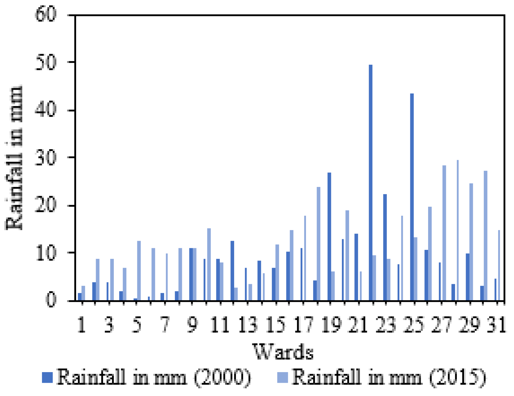
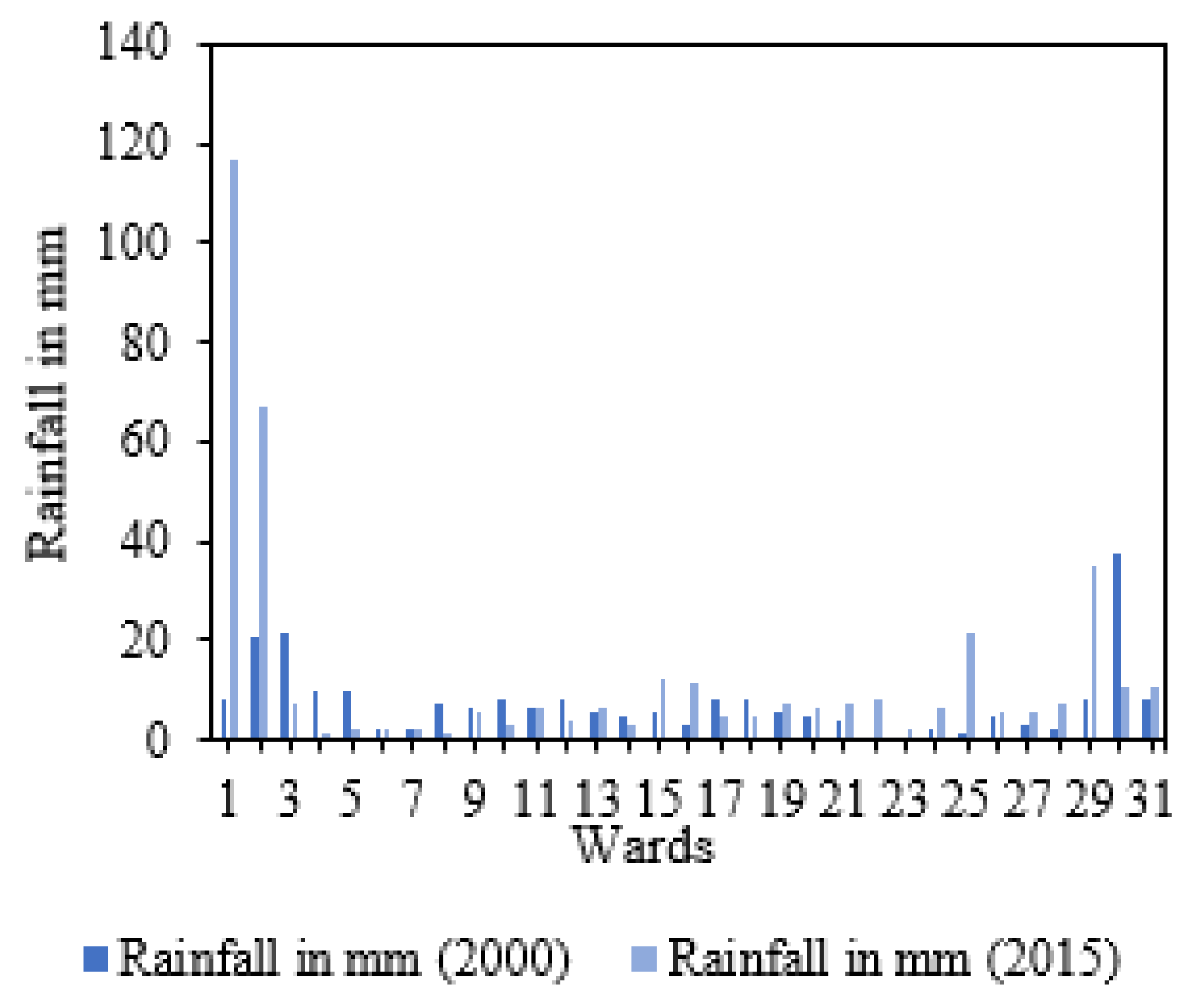
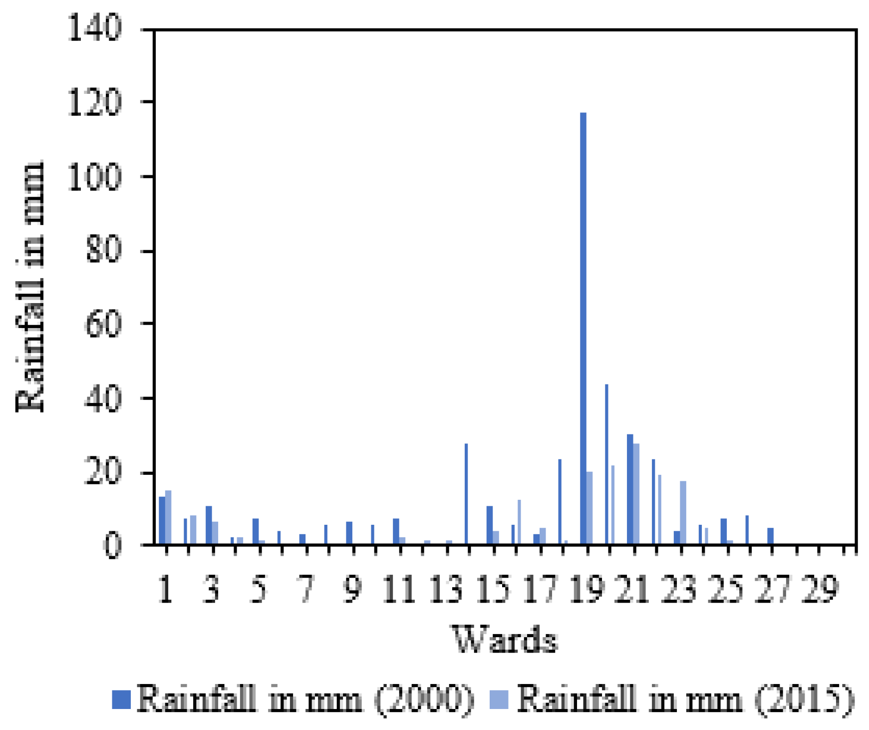
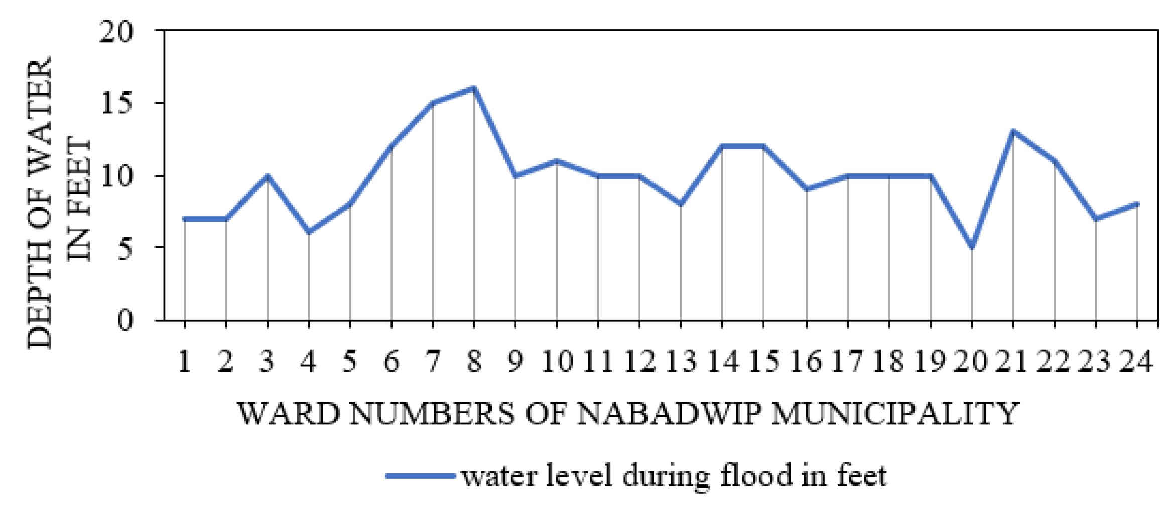
4.1. An Outline of Rainfall Situation and Flood Occurrences in Nabadwip Municipality
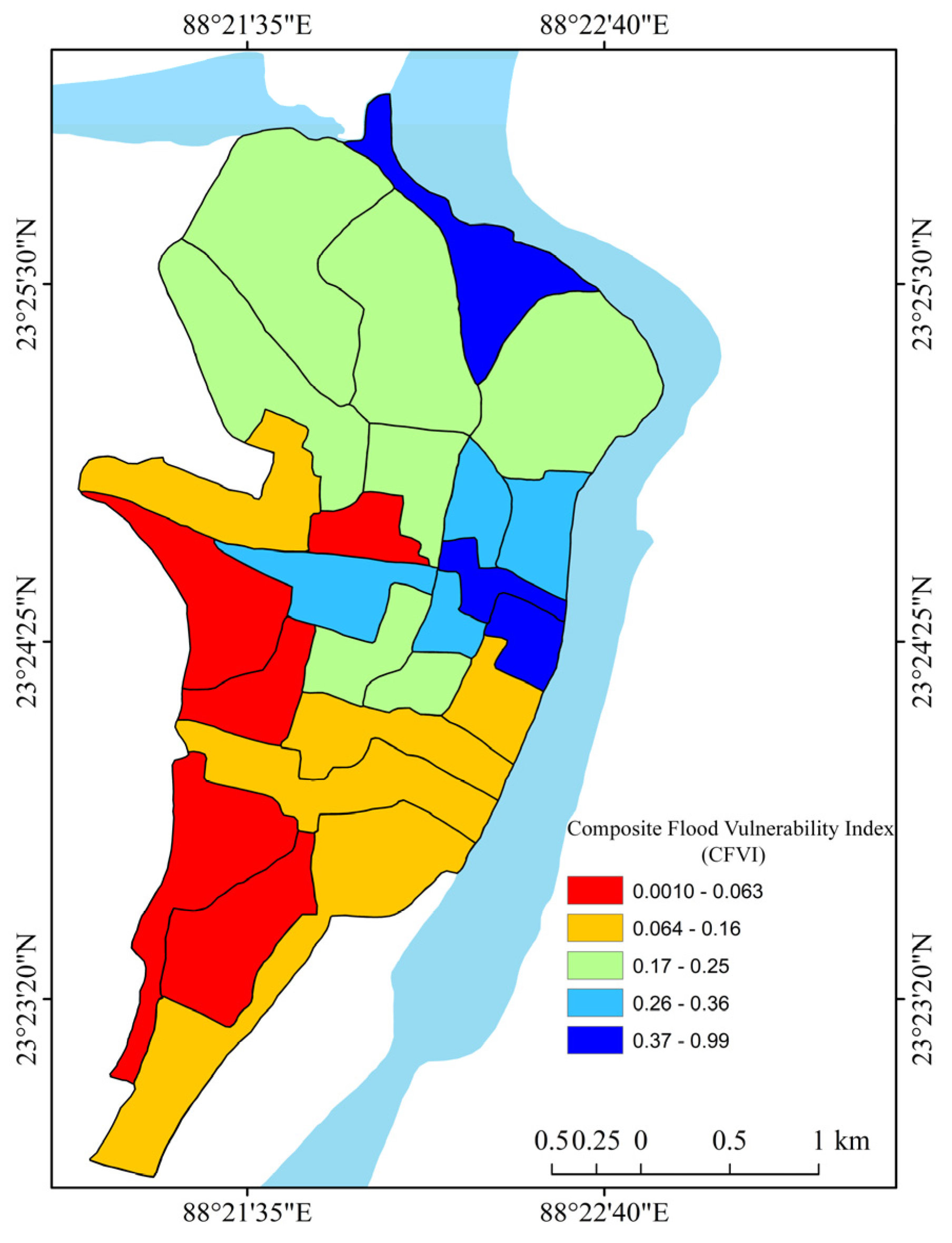
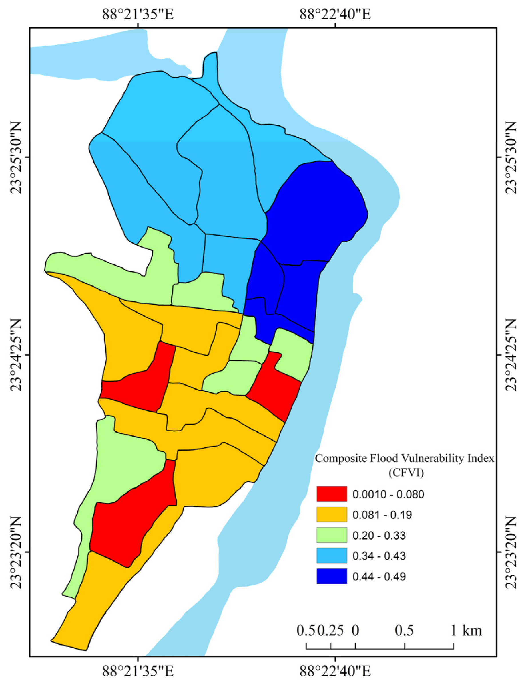
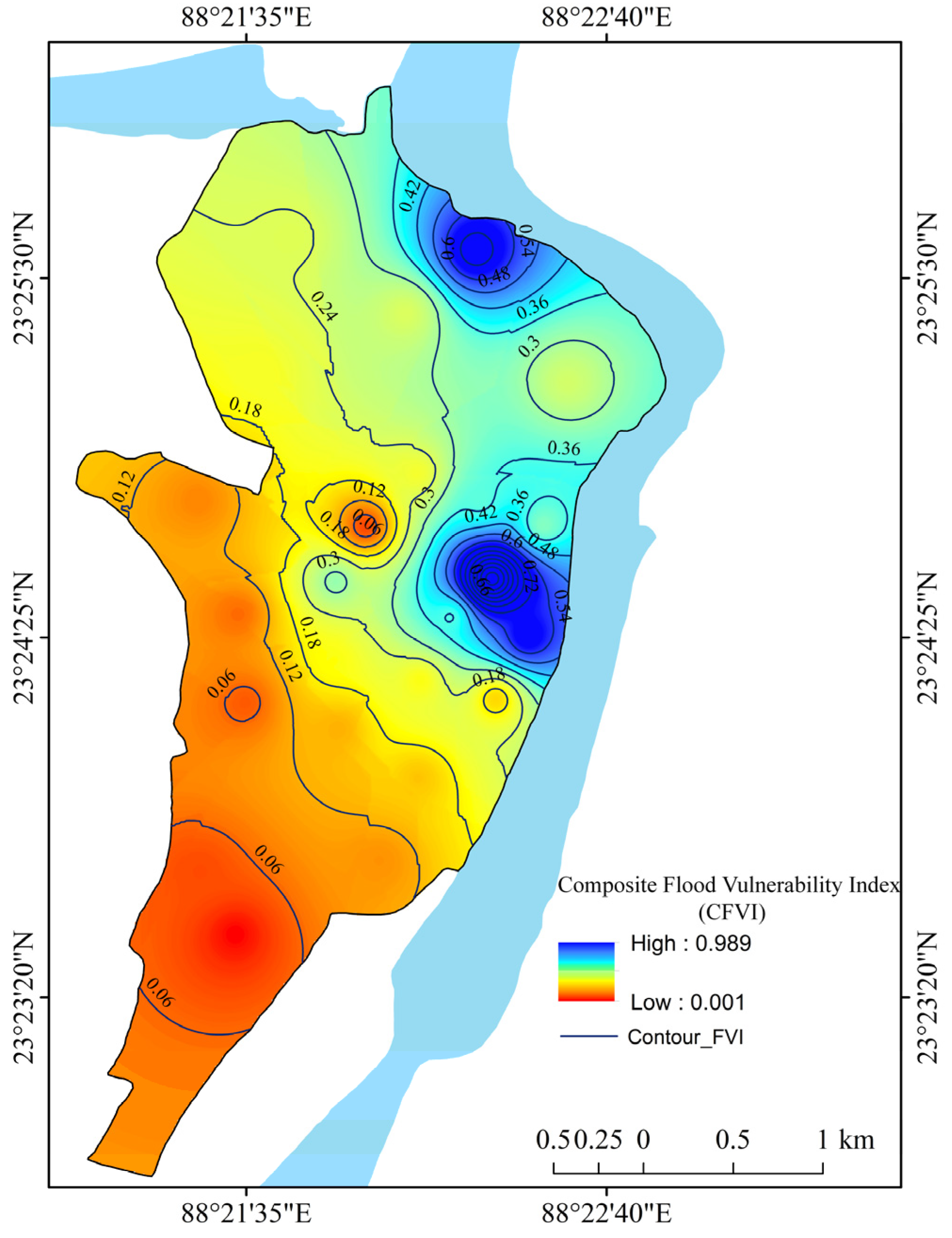
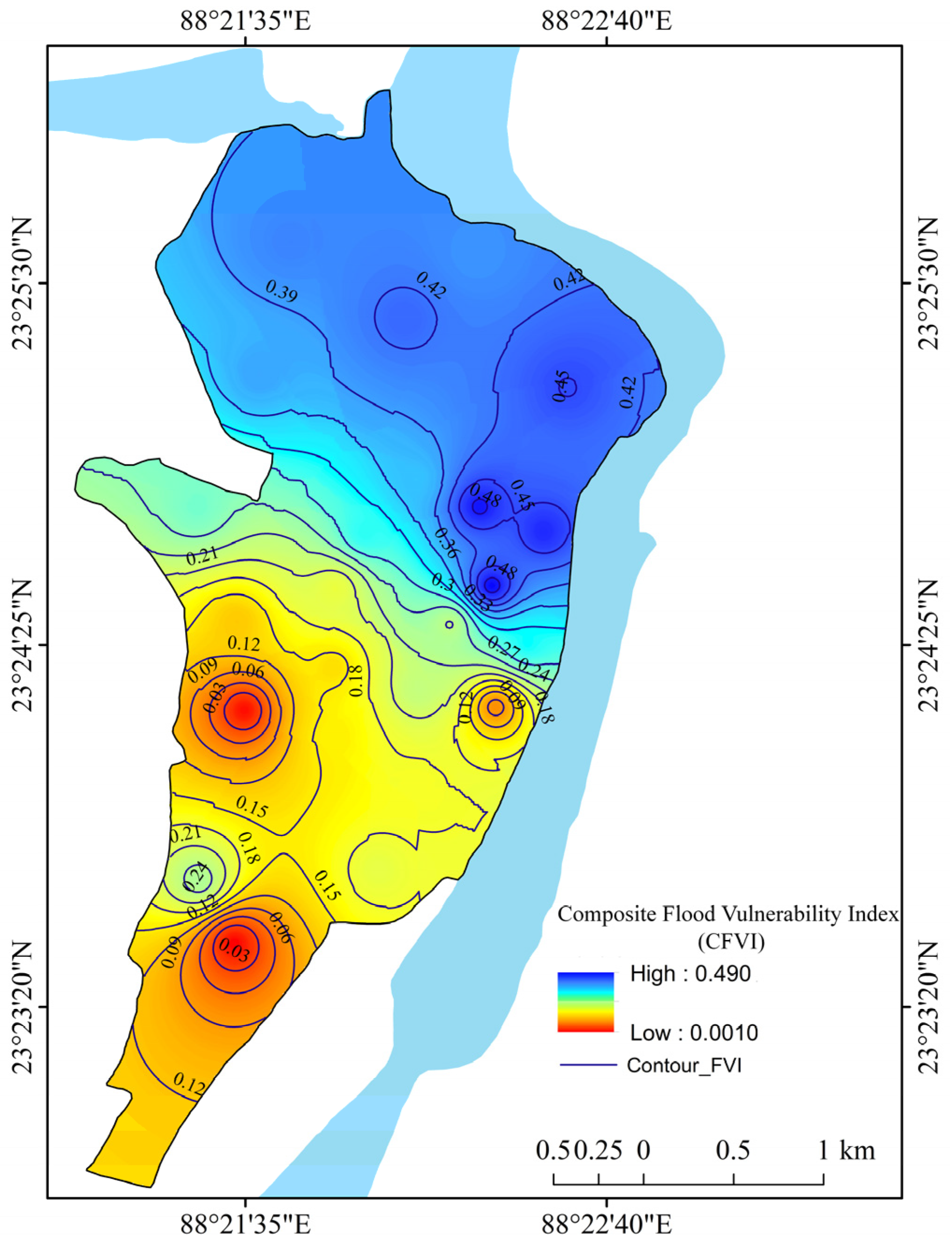
4.2. Factors and Zonation of Flood Vulnerability
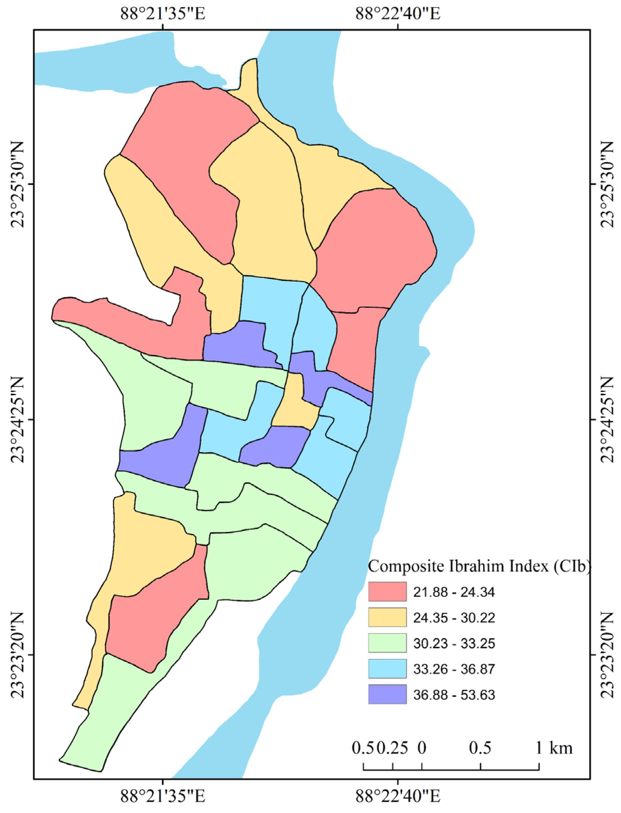
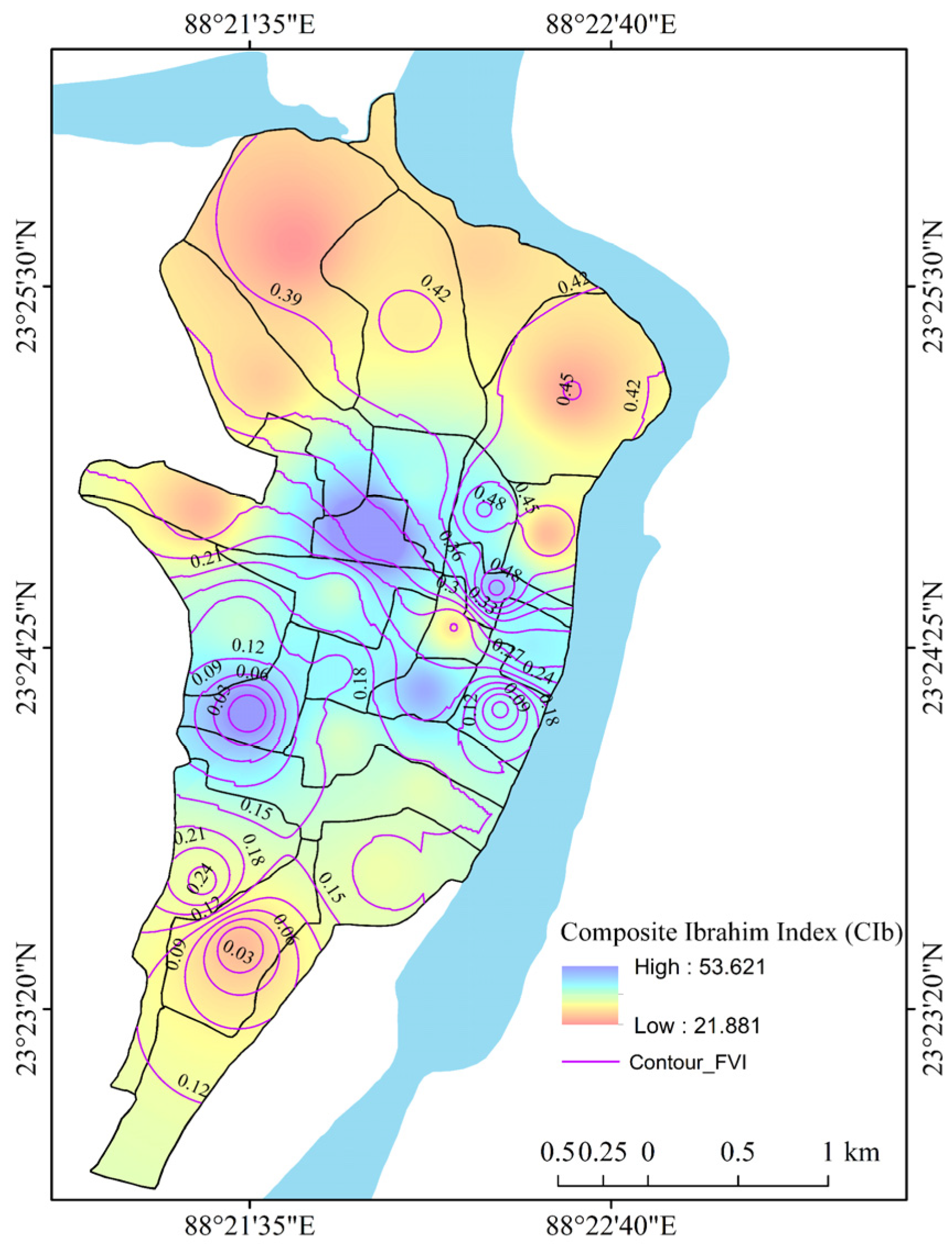
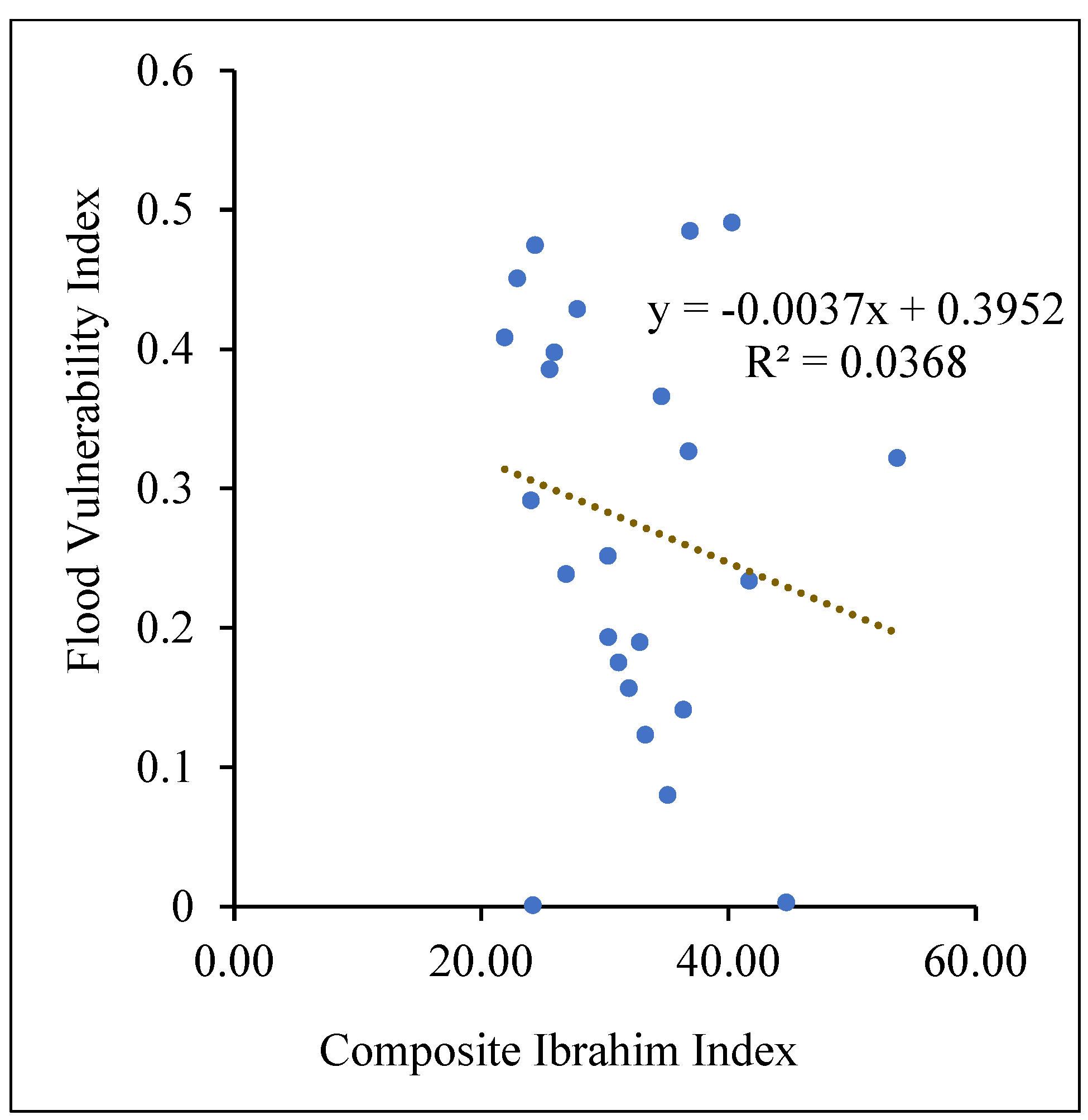
4.3. Relationship between Urban Development and Flood Vulnerability
5. Major Findings, Discussion, and Policy Suggestions
6. Conclusions
Author Contributions
Funding
Institutional Review Board Statement
Informed Consent Statement
Data Availability Statement
Conflicts of Interest
Abbreviations
| DEM | Digital Elevation Model |
| LULC | Land Use Land Cover |
| TWI | Topographic Wetness Index |
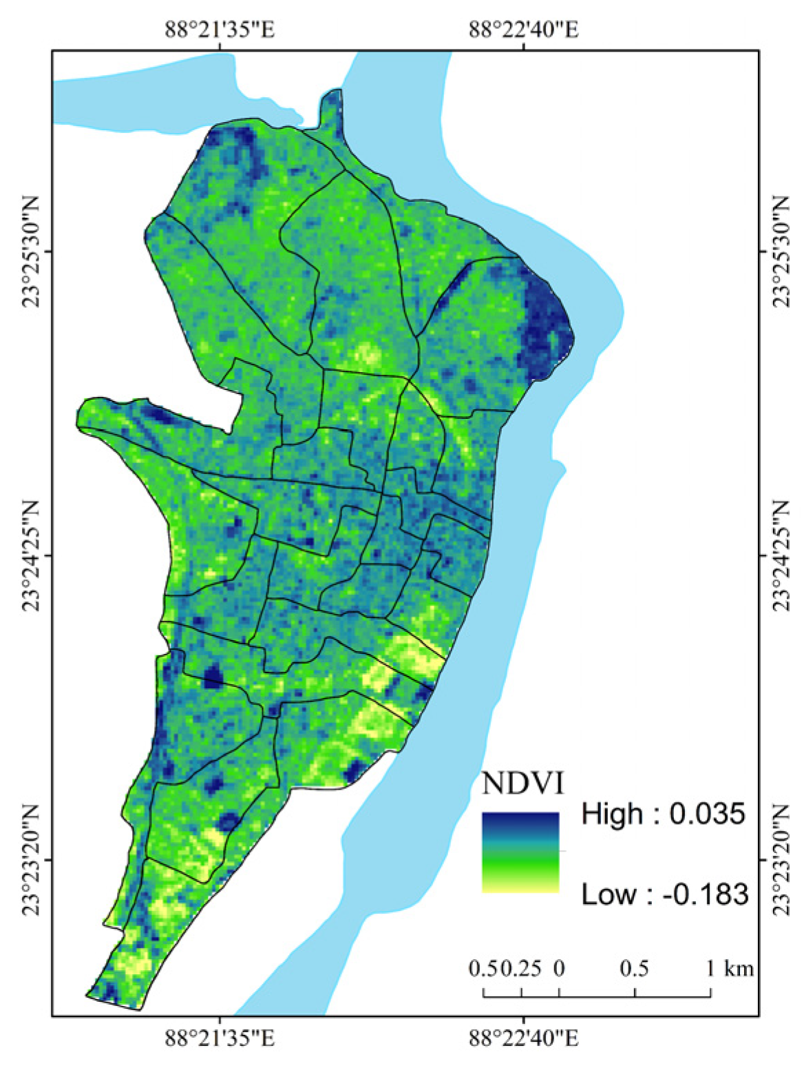
| NDVI | Normalized Difference Vegetation Index |
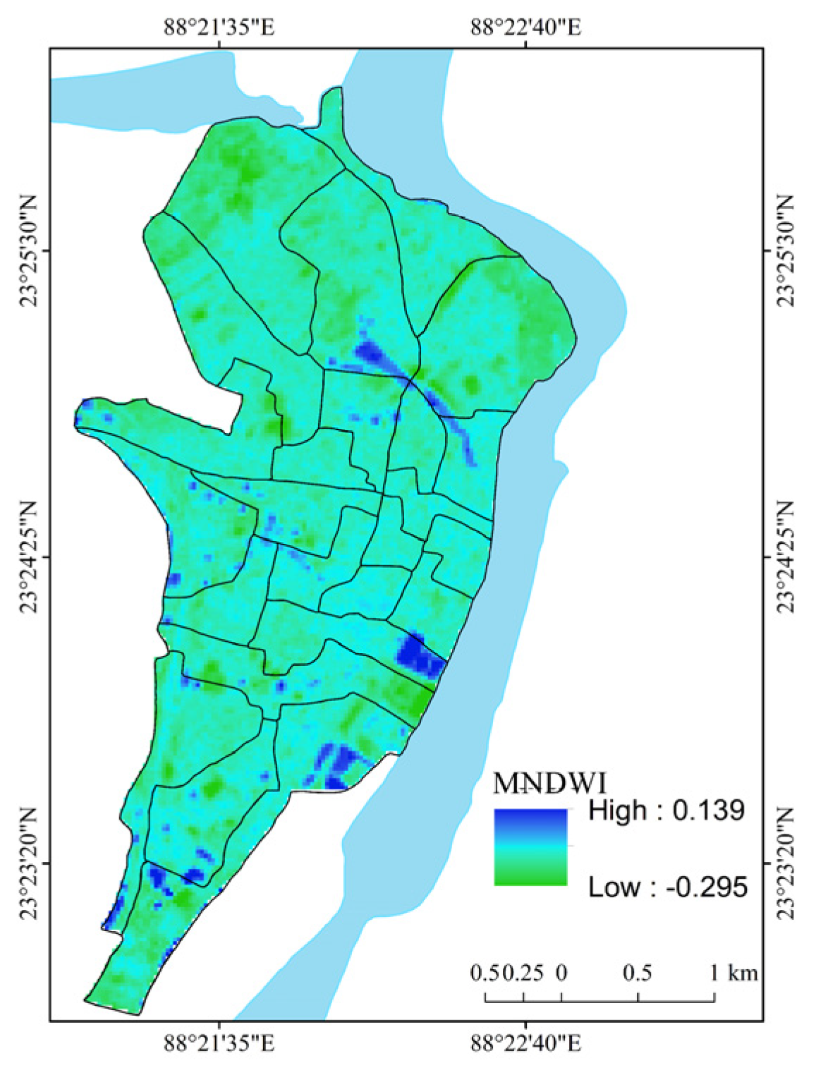
| MNDWI | Modified Normalized Difference Water Index |
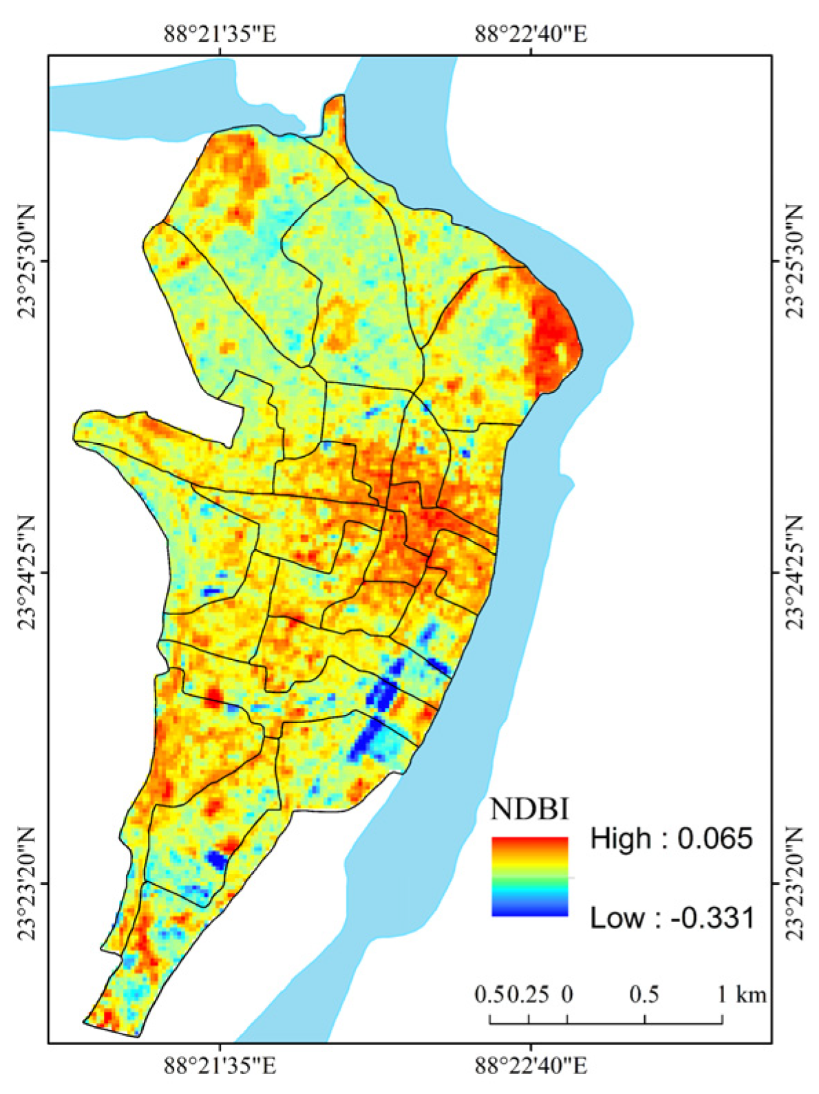
| NDBI | Normalized Difference Built-Up Index |
| SPI | Standardized Precipitation Index |
| STI | Sediment Transport Index |
| AHP | Analytical Hierarchy Process |
| MCDM | Multi-Criteria Decision Making |
| GIS | Geographic Information System |
| F-AHP | Fuzzy Analytical Hierarchy Process |
| M.S.L. | Mean Sea Level |
| SODA | Solar Radiation Data |
| MERRA | Modern-Era Retrospective Analysis for Research and Applications |
| NASA | National Aeronautics and Space Administration |
| USGS | United States Geological Survey |
| NRSC | National Remote Sensing Centre |
| mm | Millimeter |
| SD | Standard Deviation |
| U statistics | Unbiased Statistics |
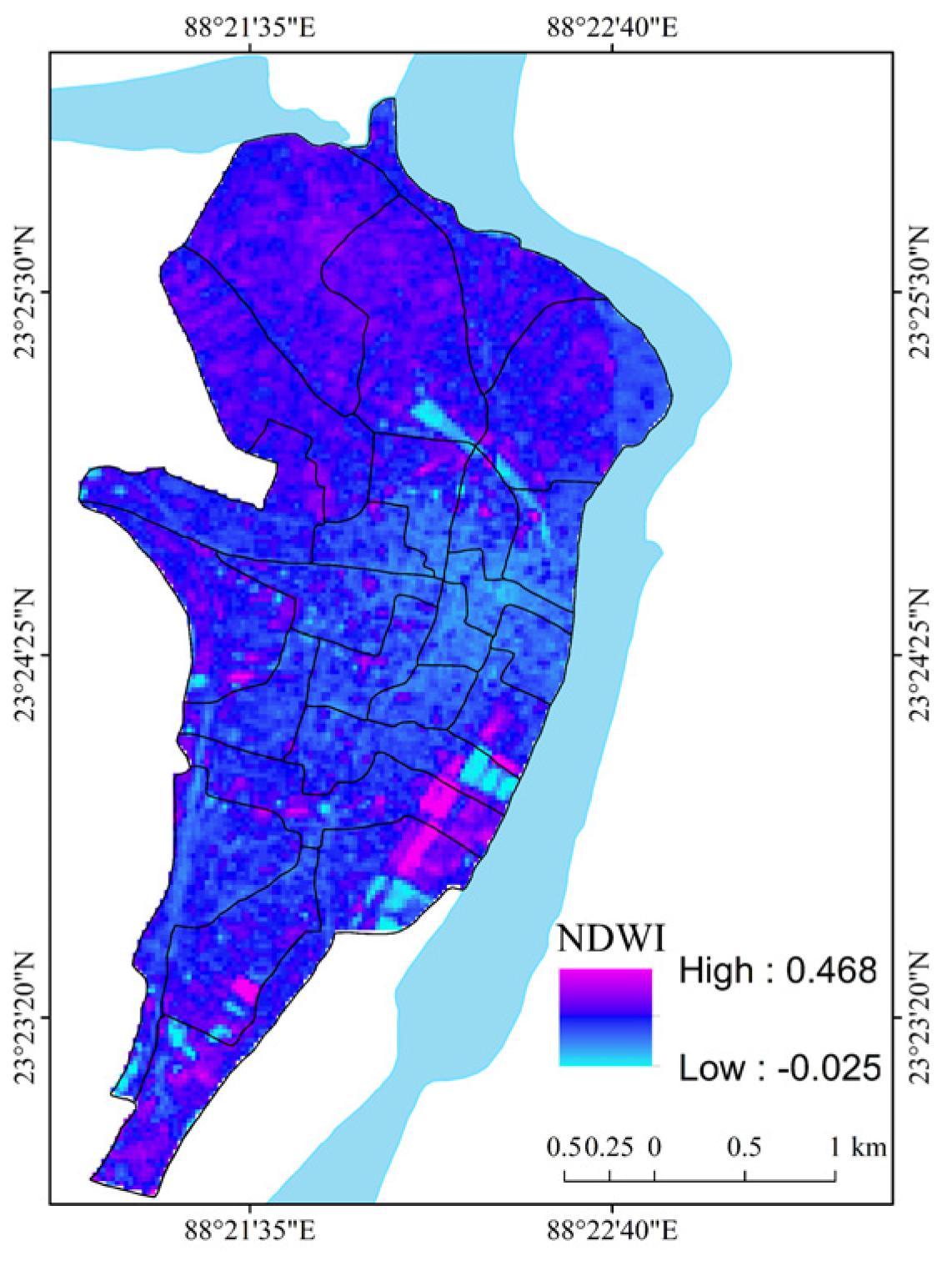
| NDWI | Normalized Difference Water Index |
| NDFI | Normalized Difference Flood Index |
| NDTI | Normalized Difference Turbidity Index |
| NDSI | Normalized Difference Soil Index |
| FVI | Flood Vulnerability Index |
| SWIR | Shortwave Infrared |
| CR | Consistency Ratio |
| CI | Consistency Index |
| RI | Random Index |
| CFVI | Composite Flood Vulnerability Index |
| CIb | Composite Ibrahim Index |
| SC | Scheduled Castes |
| ST | Scheduled Tribes |
| ANOVA | Analysis of Variance |
| ROC | Receiver Operating Characteristic |
| AUC | Area Under the ROC Curve |
| IDW | Inverse Distance Weight |
| SWOC | Strengths, Weaknesses, Opportunities, Challenges |
| SWOT | Strengths, Weaknesses, Opportunities, Threats |
| W1C1 | Weakness 1, Challenge 1 |
| O2S1 | Opportunity 2, Strength 1 |
| LMCI | Lower Mean Confidence Interval |
| UMCI | Upper Mean Confidence Interval |
| COV | Covariance |
| SRTM | Shuttle Radar Topographic Mission |
| ETM+ | Enhanced Thematic Mapper Plus |
| LISS NIR | Linear Imaging Self Scanning Near Infrared |
| Std. Deviation | Standard Deviation |
| Df | Degree of Freedom |
| Sig. | Significance |
| VIF | Variance Inflation Factor |
References
- Nkwunonwo, U.C.; Whitworth, M.; Baily, B.; Inkpen, R. The development of a simplified model for urban flood risk mitigation in developing countries. In Vulnerability, Uncertainty, and Risk: Quantification, Mitigation, and Management; American Society of Civil Engineers: Reston, VA, USA, 2014; pp. 1116–1127. [Google Scholar] [CrossRef]
- Bigi, V.; Comino, E.; Fontana, M.; Pezzoli, A.; Rosso, M. Flood vulnerability analysis in urban context: A socioeconomic sub-indicators overview. Climate 2021, 9, 12. [Google Scholar] [CrossRef]
- Kundzewicz, Z.W.; Kanae, S.; Seneviratne, S.I.; Handmer, J.; Nicholls, N.; Peduzzi, P.; Sherstyukov, B. Flood risk and climate change: Global and regional perspectives. Hydrol. Sci. J. 2014, 59, 1–28. [Google Scholar] [CrossRef] [Green Version]
- Zhou, Q.; Leng, G.; Huang, M. Impacts of future climate change on urban flood volumes in Hohhot in northern China: Benefits of climate change mitigation and adaptations. Hydrol. Earth Syst. Sci. 2018, 22, 305–316. [Google Scholar] [CrossRef] [Green Version]
- Kashyap, S.; Mahanta, R. Vulnerability aspects of urban flooding: A review. Indian J. Econ. Dev. 2018, 14, 578–586. [Google Scholar] [CrossRef]
- Gao, M.; Wang, Z.; Yang, H. Review of Urban Flood Resilience: Insights from Scientometric and Systematic Analysis. Int. J. Environ. Res. Public Health. 2022, 19, 8837. [Google Scholar] [CrossRef] [PubMed]
- Chan, S.W.; Abid, S.K.; Sulaiman, N.; Nazir, U.; Azam, K.A. systematic review of the flood vulnerability using geographic information system. Heliyon 2022, 8, e09075. [Google Scholar] [CrossRef]
- Gran Castro, J.A.; Ramos de Robles, S.L. Climate change and flood risk: Vulnerability assessment in an urban poor community in Mexico. Environ. Urban. 2019, 31, 75–92. [Google Scholar] [CrossRef]
- Tingsanchali, T.; Promping, T. Comprehensive assessment of flood hazard, vulnerability, and flood risk at the household level in a municipality area: A case study of Nan Province, Thailand. Water 2022, 14, 161. [Google Scholar] [CrossRef]
- Dewan, T.H. Societal impacts and vulnerability to floods in Bangladesh and Nepal. Weather Clim. Extremes 2015, 7, 36–42. [Google Scholar] [CrossRef] [Green Version]
- National Disaster Management Authority. National Disaster Management Guidelines: Management of Urban Flooding; Government of India: New Delhi, India, 2010; pp. 1–158.
- Prathipati, V.K.; CV, N.; Konatham, P. Inconsistency in the frequency of rainfall events in the Indian summer monsoon season. Int. J. Climatol. 2019, 39, 4907–4923. [Google Scholar] [CrossRef]
- Vazhuthi, H.I.; Kumar, A. Causes and impacts of urban floods in Indian cities: A review. Int. J. Emerg. Technol. 2020, 11, 140–147. [Google Scholar]
- Vignesh, K.S.; Anandakumar, I.; Ranjan, R.; Borah, D. Flood vulnerability assessment using an integrated approach of multi-criteria decision-making model and geospatial techniques. Model. Earth Syst. Environ. 2021, 7, 767–781. [Google Scholar] [CrossRef]
- Haque, M.N.; Siddika, S.; Sresto, M.A.; Saroar, M.M.; Shabab, K.R. Geo-spatial analysis for flash flood susceptibility mapping in the North-East Haor (Wetland) Region in Bangladesh. Earth Syst. Environ. 2021, 5, 365–384. [Google Scholar] [CrossRef]
- Vilasan, R.T.; Kapse, V.S. Evaluation of the prediction capability of AHP and F-AHP methods in flood susceptibility mapping of Ernakulam district (India). Nat. Hazards. 2022, 112, 1767–1793. [Google Scholar] [CrossRef]
- Ramkar, P.; Yadav, S.M. Flood risk index in data-scarce river basins using the AHP and GIS approach. Nat. Hazards. 2021, 109, 1119–1140. [Google Scholar] [CrossRef]
- Senan, C.P.; Ajin, R.S.; Danumah, J.H.; Costache, R.; Arabameri, A.; Rajaneesh, A.; Sajinkumar, K.S.; Kuriakose, S.L. Flood vulnerability of a few areas in the foothills of the Western Ghats: A comparison of AHP and F-AHP models. Stoch. Environ. Res. Risk Assess. 2022, 37, 527–556. [Google Scholar] [CrossRef]
- Basu, T. An Analysis of the Unevenness of Intra Regional Development of Urban Space and Associated Vulnerabilities: A Study on Nabadwip Municipality in Nadia District, West Bengal, India. IOSR J. Hum. Soc. Sci. 2017, 22, 1–17. [Google Scholar]
- Samal, N.R.; Roy, P.K.; Majumadar, M.; Bhattacharya, S.; Biswasroy, M. Six Years Major Historical Urban Floods in West Bengal State in India: Comparative Analysis Using Neuro-Genetic Model. Am. J. Water Resour. 2014, 2, 41–53. [Google Scholar] [CrossRef] [Green Version]
- Idris, S.; Dharmasiri, L.M. Urban development and the increasing trend of flood risk in Gombe metropolis, Nigeria. Int. J. Sci. Res. 2015, 5, 500–504. [Google Scholar]
- Wang, C.; Du, S.; Wen, J.; Zhang, M.; Gu, H.; Shi, Y.; Xu, H. Analyzing explanatory factors of urban pluvial floods in Shanghai using geographically weighted regression. Stoch. Environ. Res. Risk Assess. 2017, 31, 1777–1790. [Google Scholar] [CrossRef]
- Bezboruah, K.; Sattler, M.; Bhatt, A. Flooded Cities: A Comparative Analysis of Flood Management Policies in Indian states. Int. J. Water Gov. 2021, 17, 8. [Google Scholar] [CrossRef]
- Zhu, W.; Cao, Z.; Luo, P.; Tang, Z.; Zhang, Y.; Hu, M.; He, B. Urban Flood-Related Remote Sensing: Research Trends, Gaps and Opportunities. Remote Sens. 2022, 14, 5505. [Google Scholar] [CrossRef]
- Sarmah, T.; Das, S.; Narendr, A.; Aithal, B.H. Assessing human vulnerability to urban flood hazard using the analytic hierarchy process and geographic information system. Int. J. Disaster Risk Reduct. 2020, 50, 101659. [Google Scholar] [CrossRef]
- Rafiq, F.; Ahmed, S.; Ahmad, S.; Khan, A.A. Urban floods in India. Int. J. Sci. Eng. Res. 2016, 7, 721–734. [Google Scholar]
- Jha, C.V.; Bairagya, H. Flood and flood plains of West Bengal, India: A comparative analysis. Revista Geoaraguaia 2013, 3, 1–10. [Google Scholar]
- Sanyal, J.; Lu, X.X. Remote sensing and GIS-based flood vulnerability assessment of human settlements: A case study of Gangetic West Bengal, India. Hydrol. Process 2005, 19, 3699–3716. [Google Scholar] [CrossRef]
- Sanyal, J.; Lu, X.X. GIS-based flood hazard mapping at different administrative scales: A case study in Gangetic West Bengal, India. Singap. J. Trop. Geogr. 2006, 27, 207–220. [Google Scholar] [CrossRef]
- Bhattacharjee, K.; Behera, B. Determinants of household vulnerability and adaptation to floods: Empirical evidence from the Indian State of West Bengal. Int. J. Disaster Risk Reduct. 2018, 31, 758–769. [Google Scholar] [CrossRef]
- Rumbach, A. At the roots of urban disasters: Planning and uneven geographies of risk in Kolkata, India. J. Urban Aff. 2017, 39, 783–799. [Google Scholar] [CrossRef]
- Roy, U. Impact on the life of common people for the floods in coloneal period (1770 AD-1900 AD) & recent time (1995 AD-2016 AD): A case study of Nadia district, West Bengal. J. Emerg. Technol. Innov. Res. 2019, 6, 216–223. [Google Scholar]
- Khatun, R. Focus on better planning for flood disaster recovery in West Bengal: A geographical analysis. Int. J. Soc. Sci. Econ. Res. 2018, 3, 3673–3691. [Google Scholar]
- Mallick, S. Identification of fluvio-geomorphological changes and bank line shifting of river Bhagirathi-Hugli using remote sensing technique in and around of Mayapur Nabadwip area, West Bengal. Int. J. Sci. Res. 2016, 5, 1130–1134. [Google Scholar]
- Census of India. District Census Handbook Nadia, Village and Town Wise Primary Census Abstract (PCA); Directorate of Census Operations: West Bengal, India, 2011; Series 20, Part-XII A and B; pp. 1–464. Available online: https://censusindia.gov.in/pca/ (accessed on 19 March 2022).
- NASA (National Aeronautics and Space Administration). Shuttle Radar Topographic Mission (SRTM). EARTHDATA. USA.gov. 2000. Available online: https://www2.jpl.nasa.gov/srtm/ (accessed on 30 August 2022).
- NRSC (National Remote Sensing Centre). Cartosat-1; Government of India: New Delhi, India, 2015. Available online: https://bhuvan.nrsc.gov.in/home/index.php (accessed on 30 August 2022).
- USGS (United States Geological Survey). Landsat Data Access. Department of Interior; United States Geological Survey: Washington, DC, USA, 2000. Available online: https://earthexplorer.usgs.gov/ (accessed on 30 August 2022).
- NRSC (National Remote Sensing Centre). Resourcesat-1/Resoursat-2: LISS-III; Government of India: New Delhi, India, 2015. Available online: https://bhuvan.nrsc.gov.in/home/index.php (accessed on 30 August 2022).
- India Meteorological Department. Climatological Table; Ministry of Earth Sciences, Government of India: New Delhi, India, 2000.
- India Meteorological Department. Climatological Table; Ministry of Earth Sciences, Government of India: New Delhi, India, 2015. [Google Scholar]
- Global Modeling and Assimilation Office (GMAO). MERRA-2 Day and Month-wise Rainfall Data of Selected Coordinate Points in West Bengal, India; Goddard Earth Sciences Data and Information Services Center (GES DISC): Greenbelt, MD, USA, 2015. [CrossRef]
- European Commission. Copernicus European Drought Observatory (EDO). 2020. Available online: https://edo.jrc.ec.europa.eu (accessed on 1 August 2022).
- Santos, E.B.; de Freitas, E.D.; Rafee, S.A.; Fujita, T.; Rudke, A.P.; Martins, L.D.; Ferreira de Souza, R.A.; Martins, J.A. Spatio-temporal variability of wet and drought events in the Paraná River basin—Brazil and its association with the El Niño—Southern oscillation phenomenon. Int. J. Climatol. 2021, 41, 4879–4897. [Google Scholar] [CrossRef]
- Li, R.; Cheng, L.; Ding, Y.; Chen, Y.; Khorasani, K. Spatial and temporal variability analysis in rainfall using standardized precipitation index for the Fuhe Basin, China. In Proceedings of the Intelligent Computing for Sustainable Energy and Environment: Second International Conference, Shanghai, China, 12–13 September 2012; Springer: Berlin/Heidelberg, Germany, 2013; pp. 451–459. [Google Scholar]
- Guerreiro, M.J.; Lajinha, T.; Abreu, I. Flood Analysis with the Standardized Precipitation Index (SPI); Edições Universidade Fernando Pessoa: Porto, Portugal, 2007; Volume 4, pp. 1–7. [Google Scholar]
- Olanrewaju, C.C.; Reddy, M. Assessment and prediction of flood hazards using standardized precipitation index—A case study of eThekwini metropolitan area. J. Flood Risk Manag. 2022, 15, e12788. [Google Scholar] [CrossRef]
- Seiler, R.A.; Hayes, M.; Bressan, L. Using the standardized precipitation index for flood risk monitoring. Int. J. Climatol. 2002, 22, 1365–1376. [Google Scholar] [CrossRef]
- Edwards, D.C.; McKee, T.B. Characteristics of 20th Century Drought in the United States at Multiple Time Scales; Climatology Report No. 97–2; Colorado State University: Fort Collins, CO, USA, 1997; pp. 1–155. [Google Scholar]
- Naresh Kumar, M.; Murthy, C.S.; Sesha Sai, M.V.; Roy, P.S. On the use of Standardized Precipitation Index (SPI) for drought intensity assessment. Meteorol. Appl. 2009, 16, 381–389. [Google Scholar] [CrossRef] [Green Version]
- Abromowitz, M.; Stegun, I.A. Handbook of Mathematical Functions; Applied Mathematics Series; National Bureau of Standards: Washington, DC, USA, 1965.
- McKee, T.B.; Doesken, N.J.; Kleist, J. The relationship of drought frequency and duration to time scales. In Proceedings of the 8th Conference on Applied Climatology, Anaheim, CA, USA, 17–22 January 1993; Volume 17, pp. 179–183. Available online: https://climate.colostate.edu/pdfs/relationshipofdroughtfrequency.pdf (accessed on 1 August 2022).
- Smith, K.G. Standards for grading texture of erosional topography. Am. J. Sci. 1950, 248, 655–668. [Google Scholar] [CrossRef]
- Schumm, S.A. Evolution of drainage systems and slopes in badlands at Perth Amboy, New Jersey. Geol. Soc. Am. Bull. 1956, 67, 597–646. [Google Scholar]
- Wentworth, C.K. A simplified method of determining the average slope of land surfaces. Am. J. Sci. 1930, 5, 184–194. [Google Scholar] [CrossRef]
- Lemenkova, P. Flow Direction and Length Determined by ArcGIS Spatial Analyst and Terrain Elevation Data Sets. In Proceedings of the Conference ‘Priority Directions of the Development of Young Research Farmers in Modern Science’, 25th Anniversary of Caspian Research Institute of Arid Agriculture RAAS, Moscow, Russia, 11–13 May 2016; Shherbakova, N.A., Bondarenko, A.N., Eds.; PNIIAZ: Moscow, Russia, 2016; pp. 579–583. [Google Scholar]
- Martz, L.W.; Garbrecht, J. Numerical definition of drainage network and subcatchment areas from digital elevation models. Comput. Geosci. 1992, 18, 747–761. [Google Scholar] [CrossRef]
- Rouse, J.W.; Haas, R.H.; Schell, J.A.; Deering, D.W. Paper a 20. In Third Earth Resources Technology Satellite-1 Symposium: Section AB; Technical Presentations; National Aeronautics and Space Administration: Washington, DC, USA, 1973; Volume 1, p. 309. [Google Scholar]
- McFeeters, S.K. The use of the Normalized Difference Water Index (NDWI) in the delineation of open water features. Int. J. Remote Sens. 1996, 17, 1425–1432. [Google Scholar] [CrossRef]
- Xu, H. A study on information extraction of water body with the modified normalized difference water index (MNDWI). J. Remote Sens. 2005, 9, 589–595. [Google Scholar]
- Zha, Y.; Gao, J.; Ni, S. Use of normalized difference built-up index in automatically mapping urban areas from TM imagery. Int. J. Remote Sens. 2003, 24, 583–594. [Google Scholar] [CrossRef]
- Elhag, M.; Gitas, I.; Othman, A.; Bahrawi, J.; Gikas, P. Assessment of water quality parameters using temporal remote sensing spectral reflectance in arid environments, Saudi Arabia. Water 2019, 11, 556. [Google Scholar] [CrossRef] [Green Version]
- Lacaux, J.P.; Tourre, Y.M.; Vignolles, C.; Ndione, J.A.; Lafaye, M. Classification of ponds from high-spatial resolution remote sensing: Application to Rift Valley Fever epidemics in Senegal. Remote Sens. Environ. 2007, 106, 66–74. [Google Scholar] [CrossRef]
- Deng, Y.; Wu, C.; Li, M.; Chen, R. RNDSI: A ratio normalized difference soil index for remote sensing of urban/suburban environments. Int. J. Appl. Earth Obs. Geoinf. 2015, 39, 40–48. [Google Scholar] [CrossRef]
- Wan, K.M.; Billa, L. Post-flood land use damage estimation using improved Normalized Difference Flood Index (NDFI3) on Landsat 8 datasets: December 2014 floods, Kelantan, Malaysia. Arab. J. Geosci. 2018, 11, 434. [Google Scholar] [CrossRef]
- Boschetti, M.; Nutini, F.; Manfron, G.; Brivio, P.A.; Nelson, A. Comparative analysis of normalised difference spectral indices derived from MODIS for detecting surface water in flooded rice cropping systems. PLoS ONE 2014, 9, e88741. [Google Scholar] [CrossRef]
- Cian, F.; Marconcini, M.; Ceccato, P. Normalized Difference Flood Index for rapid flood mapping: Taking advantage of EO big data. Remote Sens. Environ. 2018, 209, 712–730. [Google Scholar] [CrossRef]
- Deepak, S.; Rajan, G.; Jairaj, P.G. Geospatial approach for assessment of vulnerability to flood in local self-governments. Geoenviron. Dis. 2020, 7, 1–19. [Google Scholar] [CrossRef]
- Taromideh, F.; Fazloula, R.; Choubin, B.; Emadi, A.; Berndtsson, R. Urban flood-risk assessment: Integration of decision-making and machine learning. Sustainability 2022, 14, 4483. [Google Scholar] [CrossRef]
- Saaty, R.W. The analytic hierarchy process—What it is and how it is used. Math. Model 1987, 9, 161–176. [Google Scholar] [CrossRef] [Green Version]
- Bozdağ, A.; Yavuz, F.; Günay, A.S. AHP and GIS based land suitability analysis for Cihanbeyli (Turkey) County. Environ. Earth Sci. 2016, 75, 813. [Google Scholar] [CrossRef]
- Saaty, T.L. A scaling method for priorities in hierarchical structures. J. Math. Psychol. 1977, 15, 234–281. [Google Scholar] [CrossRef]
- Saaty, T.L. The Analytic Hierarchy Process; Agricultural Economics Review; McGraw Hill: New York, NY, USA, 1980; Volume 70. [Google Scholar]
- Abu Dabous, S.; Alkass, S. Decision support method for multi-criteria selection of bridge rehabilitation strategy. Constr. Manag. Econ. 2008, 26, 883–893. [Google Scholar] [CrossRef]
- Bhushan, N.; Rai, K. Strategic Decision Making: Applying the Analytic Hierarchy Process; Springer: London, UK, 2004; pp. 1–170. [Google Scholar]
- Ibrahim, M. Ibrahim Index of African Governance; Data Report; Mo Ibrahim Foundation: London, UK, 2012. [Google Scholar]
- Gisselquist, R.M. Evaluating Governance Indexes: Critical and Less Critical Questions; WIDER Working Paper Series wp-2013-068; World Institute for Development Economic Research (UNU-WIDER): Helsinki, Finland, 2013. [Google Scholar]
- Uyanık, G.K.; Güler, N. A study on multiple linear regression analysis. Procedia Soc. Behav. Sci. 2013, 106, 234–240. [Google Scholar] [CrossRef] [Green Version]
- Pearson, K. VII. Mathematical Contributions to the Theory of Evolution—III. Regression, Heredity, and Panmixia; University College London: London, UK, 1896; Volume 187, pp. 253–318. Available online: http://rsta.royalsocietypublishing.org/content/187/253.full.pdf (accessed on 1 August 2022)Containing Papers of a Mathematical or Physical Character.
- Pearson, K. On certain errors with regard to multiple correlation occasionally made by those who have not adequately studied this subject. Biometrika 1914, 10, 181–187. Available online: http://www.jstor.org/stable/2331747 (accessed on 1 August 2022).
- Durbin, J.; Watson, G.S. Testing For Serial Correlation in Least Squares Regression. III. Biometrika 1971, 58, 1–19. [Google Scholar] [CrossRef]
- Farebrother, R.W. The Durbin-Watson test for serial correlation when there is no intercept in the regression. Econometrica 1980, 48, 1553–1563. [Google Scholar] [CrossRef]
- Holt, W.; Refenes, P. The Durbin-Watson test for neural regression models. In Risk Measurement, Econometrics and Neural Networks: Selected Articles of the 6th Econometric-Workshop in Karlsruhe, Germany; Physica-Verlag HD: Heidelberg, Germany, 1998; pp. 57–68. [Google Scholar] [CrossRef]
- Fisher, R.A. Statistical Methods for Research Workers; Oliver and Boyd London and Edinburgh (§4 and §42 (Ex. 41) Reproduced; Springer: Berlin/Heidelberg, Germany, 1934. [Google Scholar]
- Welch, B.L. The generalization of ‘student’s’ problem when several different population variances are involved. Biometrika 1947, 34, 28–35. [Google Scholar] [CrossRef] [PubMed]
- Nam, B.H.; D’Agostino, R.B. Discrimination index, the area under the ROC curve. In Goodness-of-Fit Tests and Model Validity; Huber-Carol, C., Balakrishnan, N., Nikulin, M.S., Mesbah, M., Eds.; Birkhäuser Boston: Boston, MA, USA, 2002; pp. 267–279. [Google Scholar]
- Grimnes, S.; Martinsen, Ø.G. Bioimpedance and Bioelectricity Basics; Elsevier: Amsterdam, The Netherlands, 2015; pp. 329–404. [Google Scholar] [CrossRef]
- Khosravi, K.; Pourghasemi, H.R.; Chapi, K.; Bahri, M. Flash flood susceptibility analysis and its mapping using different bivariate models in Iran: A comparison between Shannon’s entropy, statistical index, and weighting factor models. Environ. Monit. Assess. 2016, 188, 1–21. [Google Scholar] [CrossRef] [PubMed]
- Farhadi, H.; Najafzadeh, M. Flood risk mapping by remote sensing data and random forest technique. Water 2021, 13, 3115. [Google Scholar] [CrossRef]
- Saha, A.K.; Agrawal, S. Mapping and assessment of flood risk in Prayagraj district, India: A GIS and remote sensing study. Nanotechnol. Environ. Eng. 2020, 5, 1–18. [Google Scholar] [CrossRef]
- Irrigation and Waterways Directorate. Annual Flood Report 2000; Government of West Bengal: West Bengal, India, 2000; pp. 1–17.
- Irrigation and Waterways Directorate. Annual Flood Report for the Year 2015; Advance Planning, Project Evaluation & Monitoring Cell; Government of West Bengal: West Bengal, India, 2015; pp. 1–57.
- Binns, A.D. Flood mitigation measures in an era of evolving flood risk. J. Flood Risk Manag. 2020, 13, e12659. [Google Scholar] [CrossRef]
- van Doorn-Hoekveld, W.; Groothuijse, F. Analysis of the strengths and weaknesses of Dutch water storage areas as a legal instrument for flood-risk prevention. J. Eur. Environ. Plan Law 2017, 14, 76–97. [Google Scholar] [CrossRef] [Green Version]
- Grama, V.; Avanzi, A.; Nistor-Lopatenco, L. SWOT principle in flood risk management. J. Eng. Sci. 2021, 15, 125–137. [Google Scholar] [CrossRef]
- Noorhashirin, H.; Juni, M.H. Assessing Malaysian disaster preparedness for flood. Int. J. Public Health Clin. Sci. 2016, 3, 1–5. [Google Scholar]


| Conceptual Background | Literature Review | Sources |
|---|---|---|
| Analytical approaches to urban flooding and the assessment of vulnerability | The focus of current research is on measuring flood risk in urban areas around the world using remote sensing and GIS. Analytical hierarchy processes with geographic information systems are one of the methods most frequently used to assess flood hazard vulnerability. | [24,25] |
| Urban flood scenarios in India | The urban areas were severely impacted by large urban floods that were primarily raised by heavy rain in Mumbai (on 26 July 2005), Kolkata (30 June 2007), and Chennai (in November and December 2015). | [26] |
| Studies on flood occurrences in West Bengal | West Bengal has annual flood potential areas that constitute 29.84% of the state’s total geographical area. Bardhhaman (undivided), Birbhum, Murshidabad, Nadia, Hugli, and Midnapore (undivided) were the major flood-prone areas of West Bengal. | [27] |
| Flood vulnerability assessment in West Bengal | Studies using remote sensing data and GIS analysis revealed that the districts of Nadia and Bardhaman contained a high concentration of settlements that were extremely susceptible to flooding from 1991 to 2000. According to the micro-level administrative scale, Nabadwip in the Nadia district was situated in a high-severity hazard-prone zone in Gangetic West Bengal. | [28,29] |
| Determinants of vulnerability and adaptation to floods in West Bengal | In the Murshidabad district of West Bengal, one of the main border districts of Nadia, significant household-level determinants predicted livelihood vulnerability based on exposure to flood sensitivity and adaptive capacity. | [30] |
| Urban development and flood disaster in Kolkata | The risks of flooding in Kolkata, the capital of West Bengal, have increased as a result of the legacy of poor planning and an uneven distribution of geographic elements. | [31] |
| Flood occurrences in Nadia district in West Bengal | Over the past few years, the district of Nadia has experienced major floods (1995–2000). According to a report from 20 August 2015, the flood incident had an impact on 21,508 residents of Nabadwip city. The majority of them were engaged in agriculture and household industries. | [32] |
| Flood resilience in West Bengal | A comprehensive and well-developed plan for flood recovery needs to be implemented while focusing on the flood mitigation strategies in West Bengal. | [33] |
| Sl. No. | Available Data | Date | Source(s) | Methods and Techniques | Web Links |
|---|---|---|---|---|---|
| 1 | (Shuttle Radar Topographic Mission) SRTM-DEM: SRTM1 Arc-Second Global | 2 November 2000 | [36] | Digital elevation model (DEM), slope analysis, drainage analysis | https://www.earthdata.nasa.gov/sensors/srtm (accessed on 30 August 2022) |
| 2 | CARTOSAT DEM (Cartosat-1) | 17 April 2015 and 29 April 2015 | [37] | Digital elevation model (DEM), slope analysis, drainage analysis | https://bhuvan-app3.nrsc.gov.in/data/download/index.php (accessed on 30 August 2022) |
| 3 | LANDSAT ETM+ (Enhanced Thematic Mapper Plus) | 17 November 2000 | [38] | Normalized difference spectral indices | https://earthexplorer.usgs.gov/ (accessed on 30 August 2022) |
| 4 | Resourcesat-1/Resourcesat-2: LISS-III (Linear Imaging Self Scanning) | 28 November 2015 | [39] | Normalized difference spectral indices | https://bhuvan-app3.nrsc.gov.in/data/download/index.php (accessed on 30 August 2022) |
| 5 | Rainfall (mm) | 1986–2015 (January to December) | [40,41,42] | Standardized precipitation index | https://mausam.imd.gov.in/ Website of Solar Radiation Data (SODA): Modern-Era Retrospective Analysis for Research and Applications (MERRA) Project collaboration with NASA (https://gmao.gsfc.nasa.gov/reanalysis/MERRA-2/) (accessed on 30 May 2022) |
| Indicators | Measurement | Source(s) | Justification for Selection |
|---|---|---|---|
| Standardized Precipitation Index (SPI) | The detailed formula has been mentioned in the Section 3. | [49] | Standardized precipitation index for analyzing monthly/annual drought conditions. |
| Relief (R) in m (1 m = 3.28084 feet) | Derived from Digital Elevation Model (DEM) | [53,54] | Terrain analysis and relief aspect of the morphometry of drainage basin. |
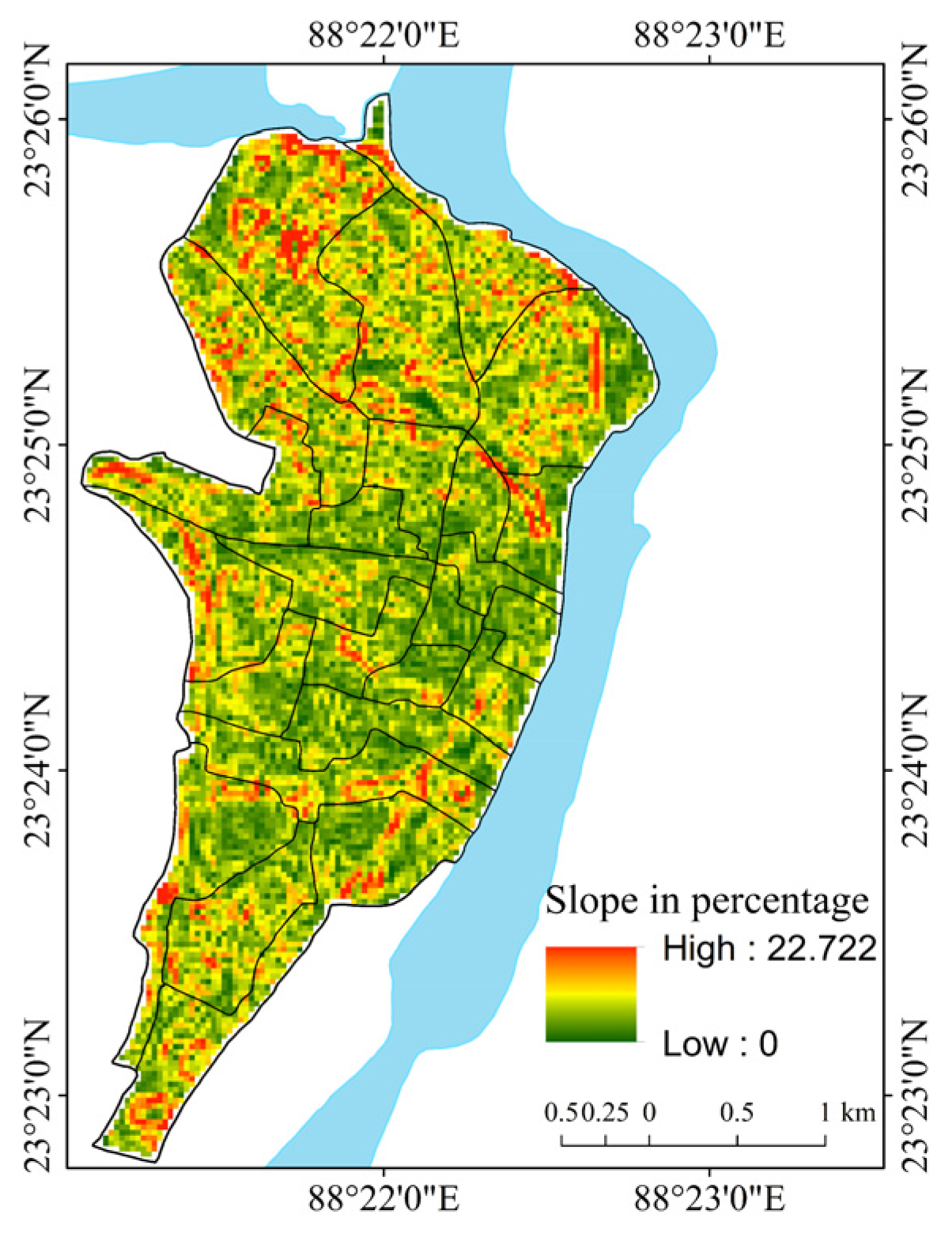
| Slope (S) in % | S = (Z × (Ctl/H))/(10 × A), basin area (A), total basin relief (H), the maximum height of the basin (Z) and total contour length, the average angle of slope (tanÕ) = Average No. of contour crossings per mile (A) × contour interval (I) 3361 (constant) | [55] | Terrain analysis and relief aspect of the morphometry of drainage basin. |
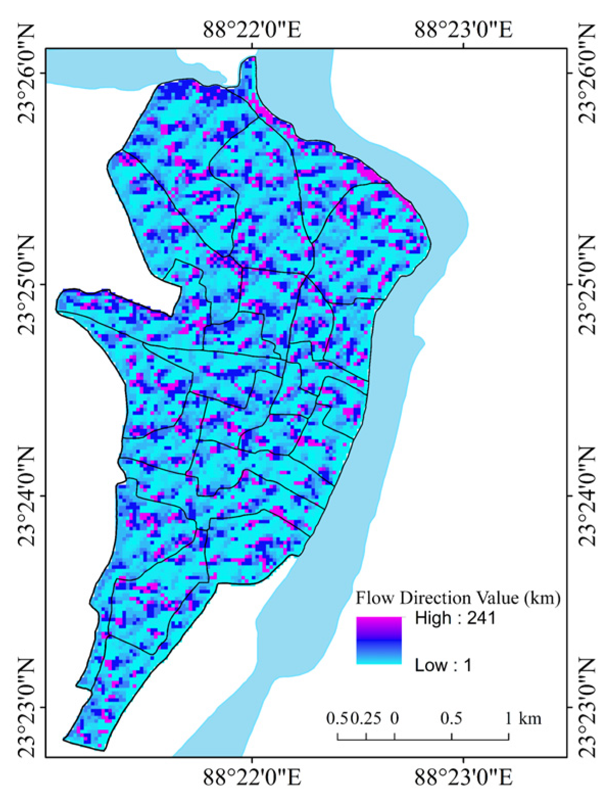
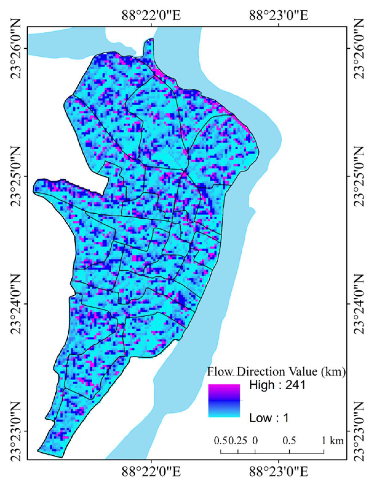
| Flow direction (Fdir) | Derived from DEM | [56,57] | The linear aspect of the flow of the drainage basin. |
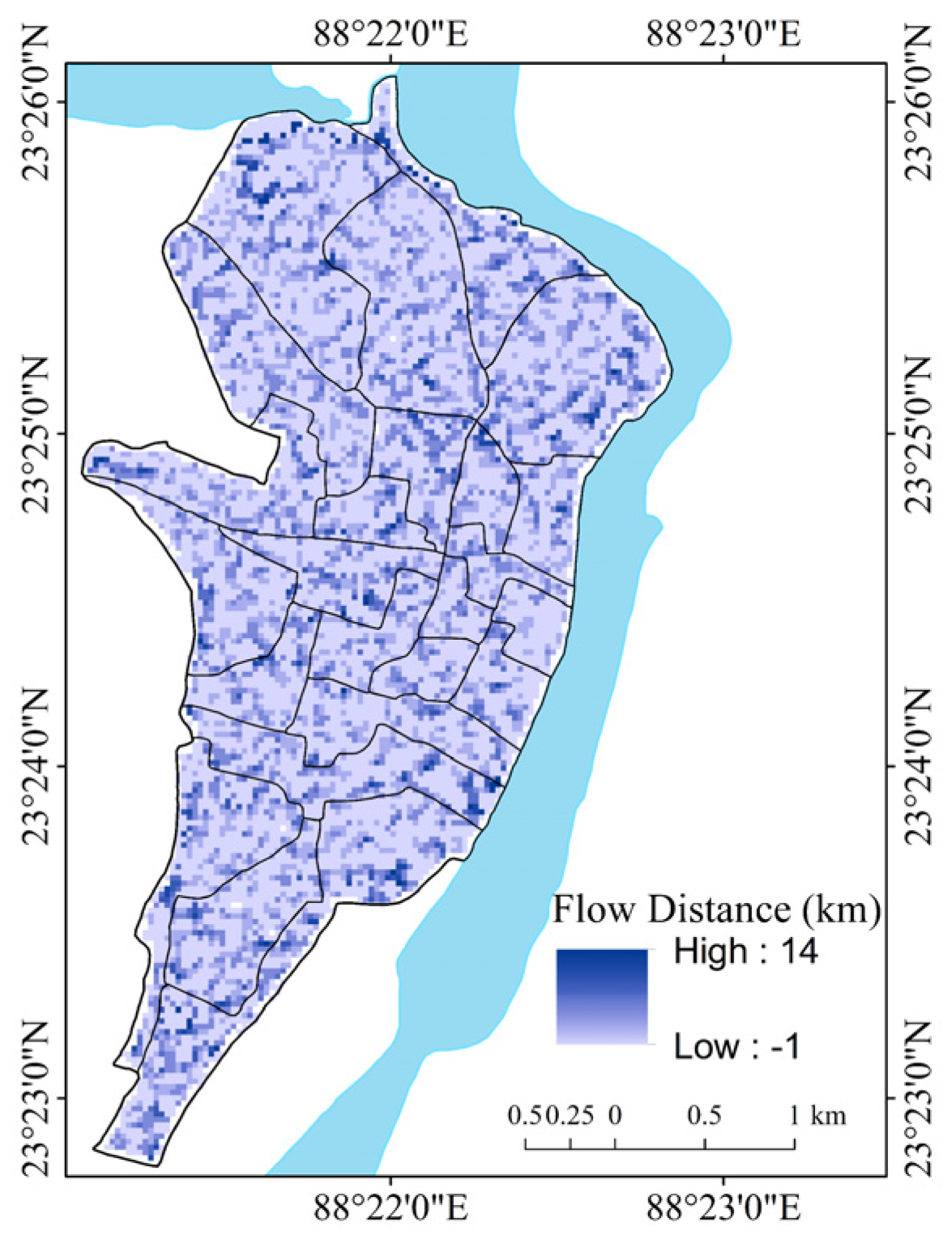
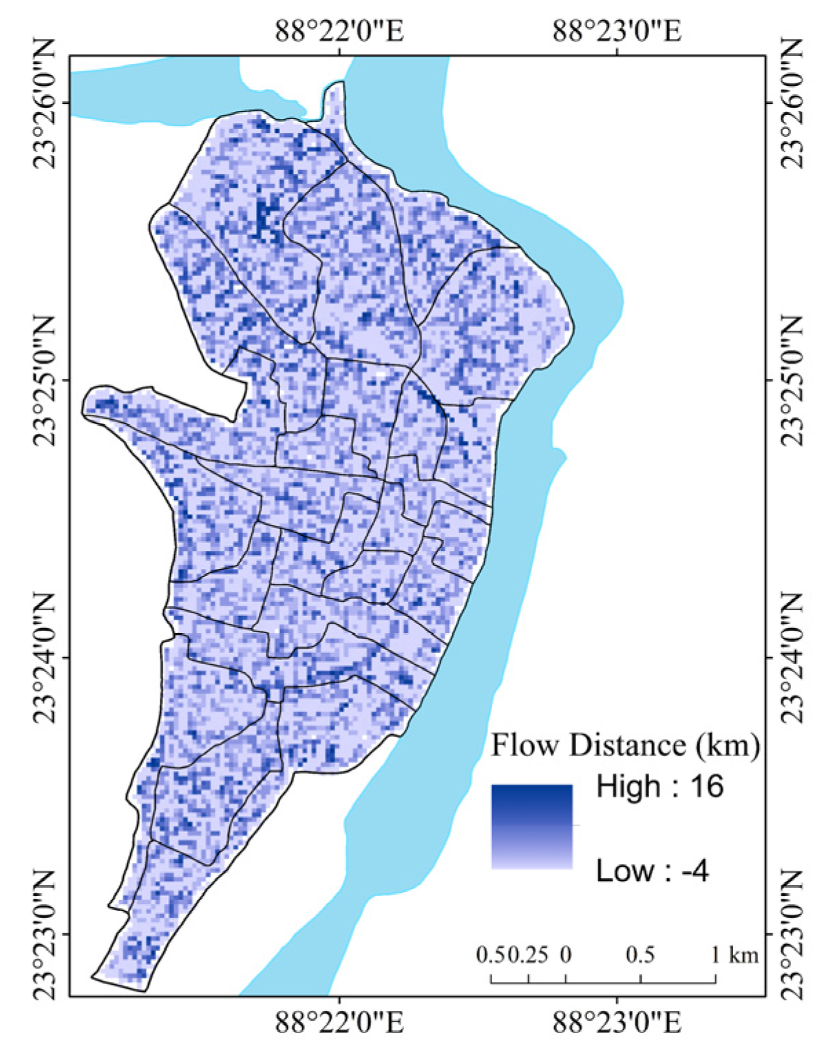
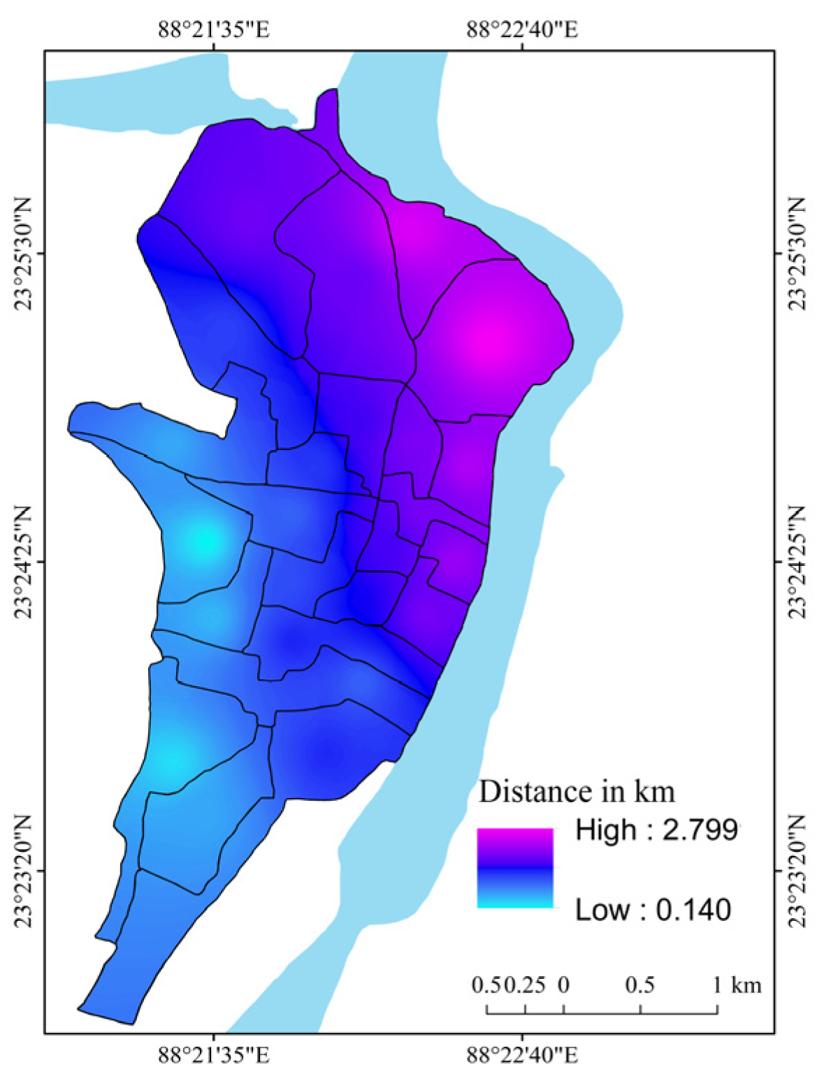
| Flow distance (Fdist) in km (0.621371 miles) | Derived from DEM | Spatial analyst in GIS | The linear aspect of the flow of the drainage basin. |
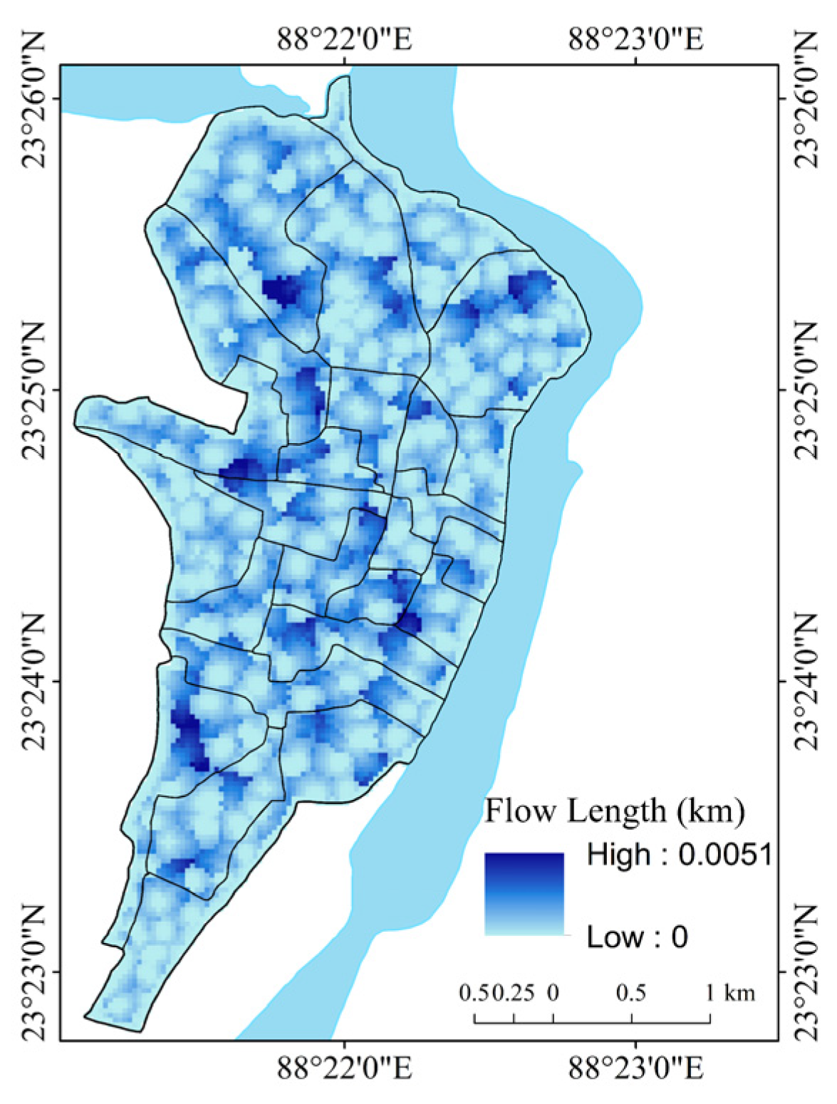
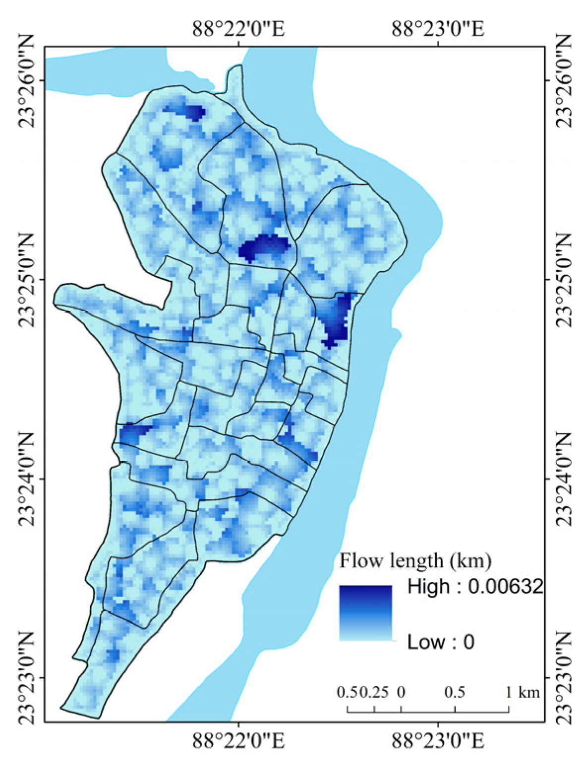
| Flow length in km (Fl) (0.621371 miles) | Derived from stream raster | [56] | The linear aspect of the flow of the drainage basin. |
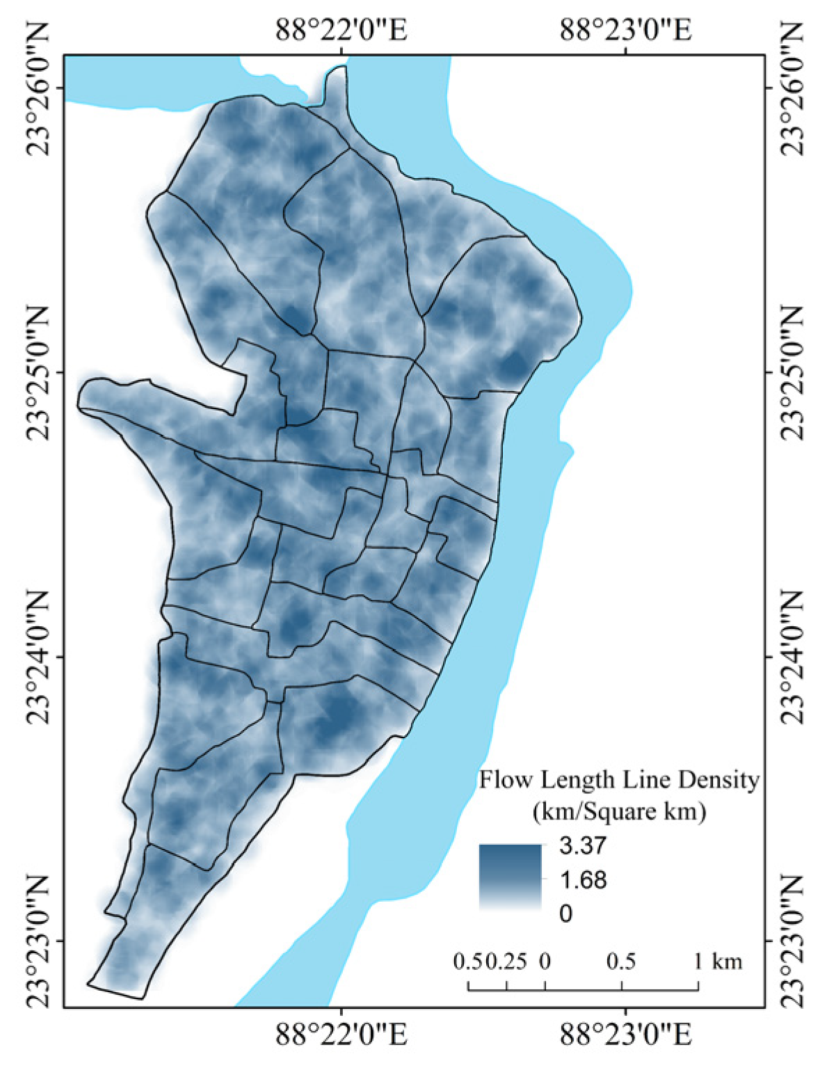
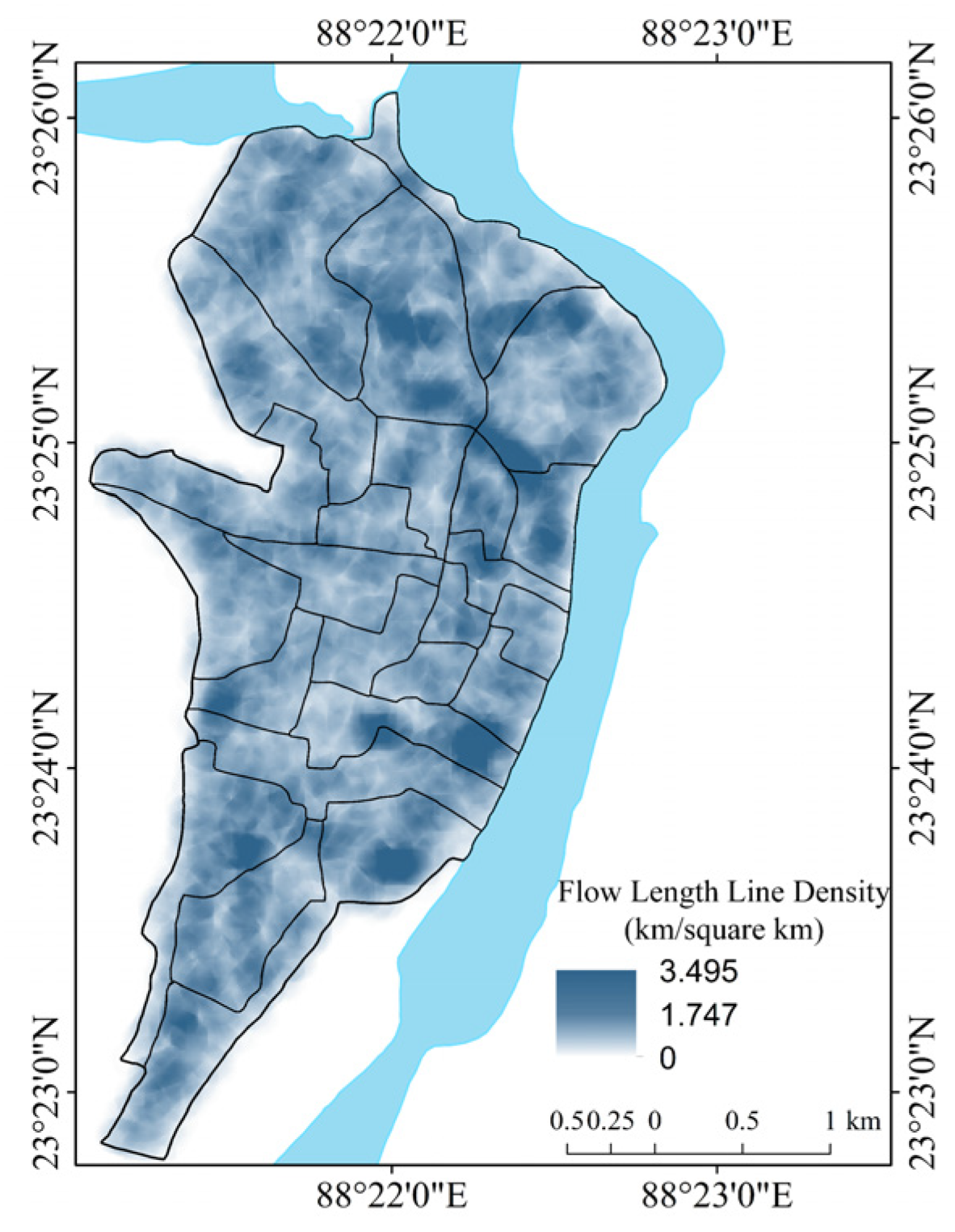
| Flow length line density (Fld) in km/square km (0.621371 mile/0.38610191964 square mile) | Derived from stream raster using line density feature in GIS analysis | Spatial analyst in GIS | The areal aspect of the flow of the drainage basin. |
| Normalized Difference Vegetation Index (NDVI) | NDVI = | [58] | Satellite imagery-based spectral index of vegetation conditions. |
| Normalized Difference Water Index (NDWI) | NDWI = | [59] | Satellite imagery-based spectral index of surface water conditions. |
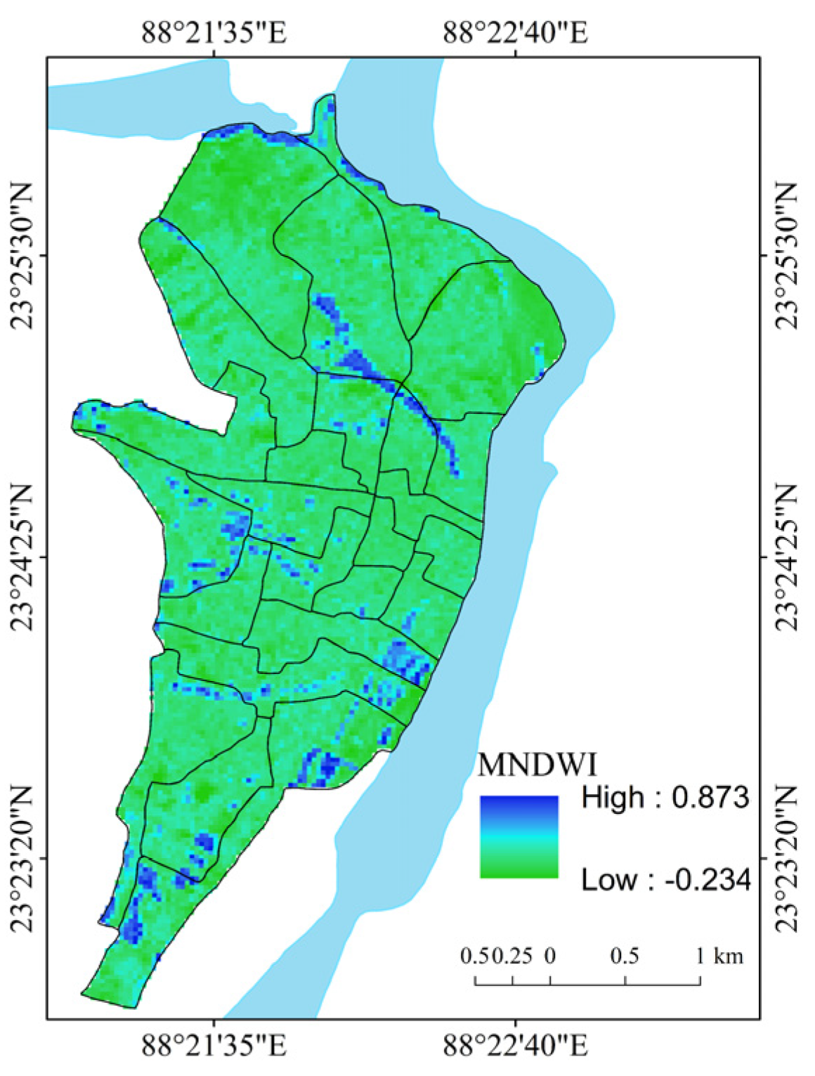
| Modified Normalized Difference Water Index (MNDWI) | MNDWI = | [60] | Satellite imagery-based spectral index of surface water conditions. |
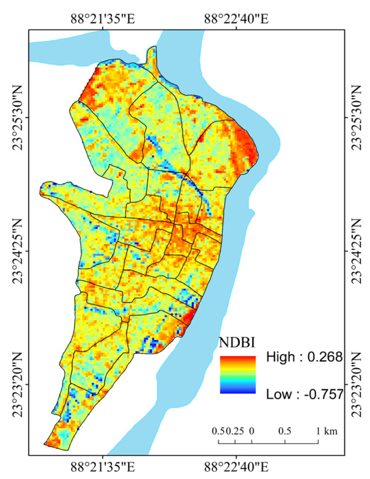
| Normalized Difference Built-Up Index (NDBI) | NDBI = | [61] | Satellite imagery-based spectral index of habitation conditions. |
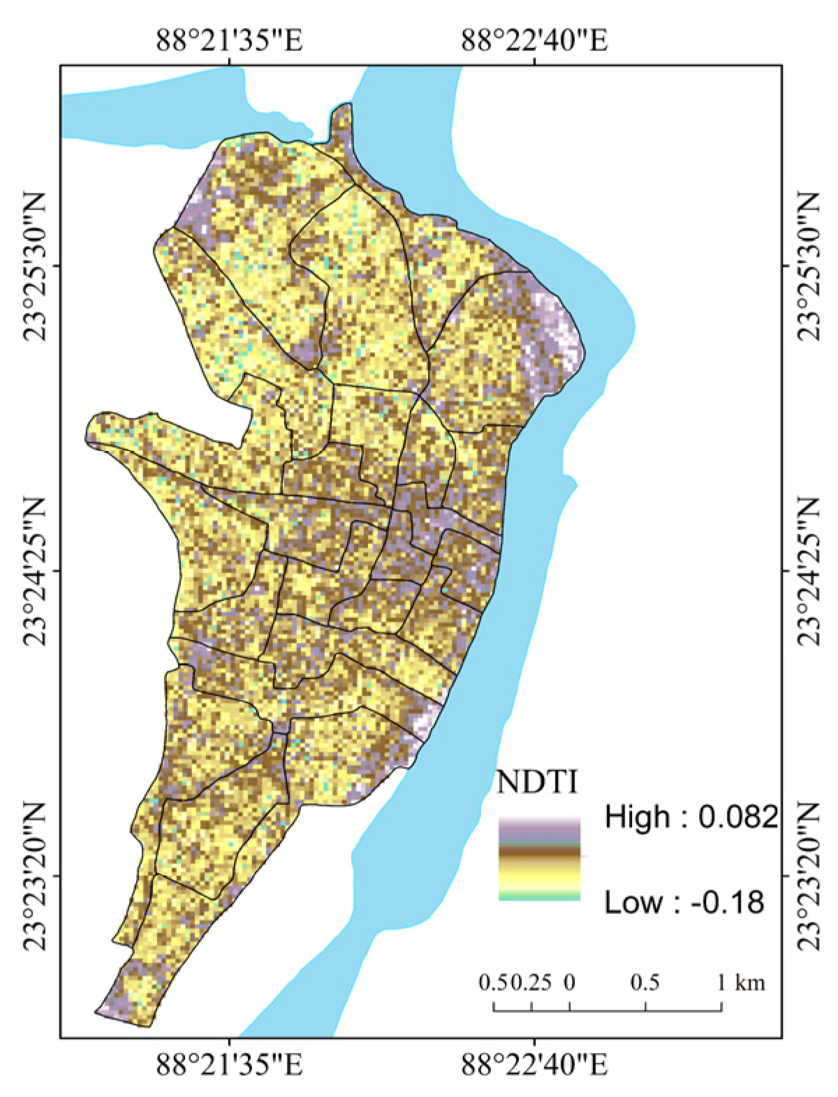
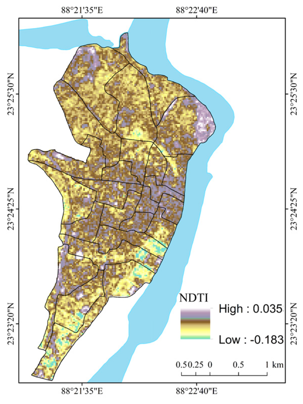
| Normalized Difference Turbidity Index (NDTI) | NDTI = | [62,63] | Satellite imagery-based spectral index of the relative clarity conditions of rivers. |
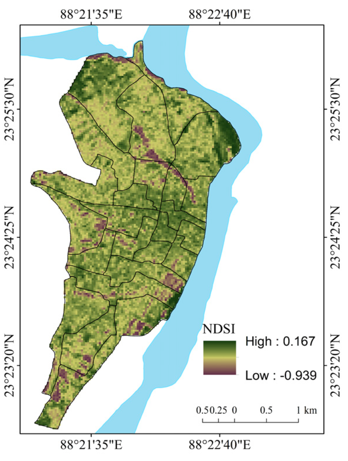
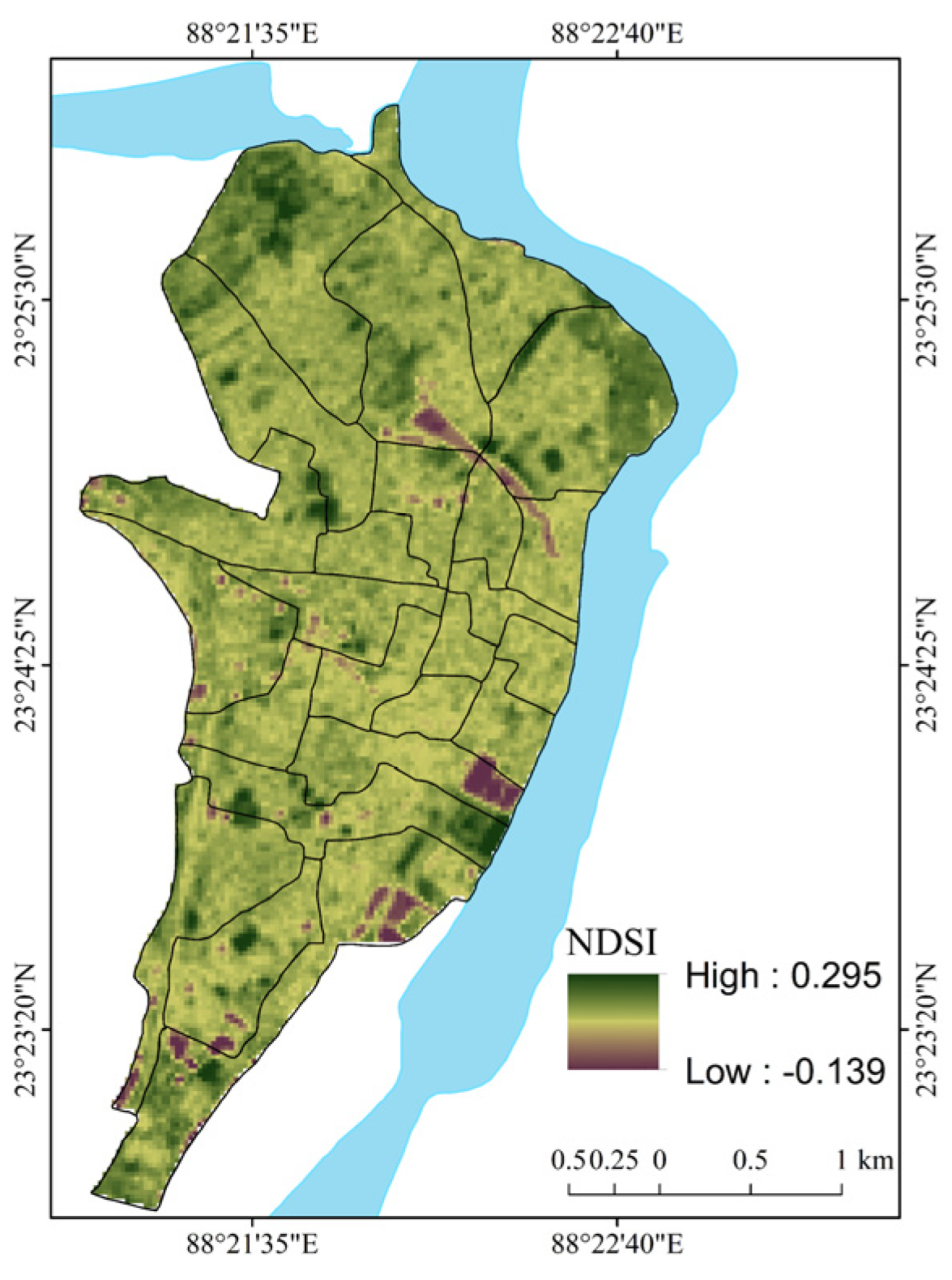
| Normalized Difference Soil Index (NDSI) | NDSI = (For ETM+ Band7 = SWIR2 and Band2 = Green.) | [64] | Satellite imagery-based spectral index of soil conditions. |
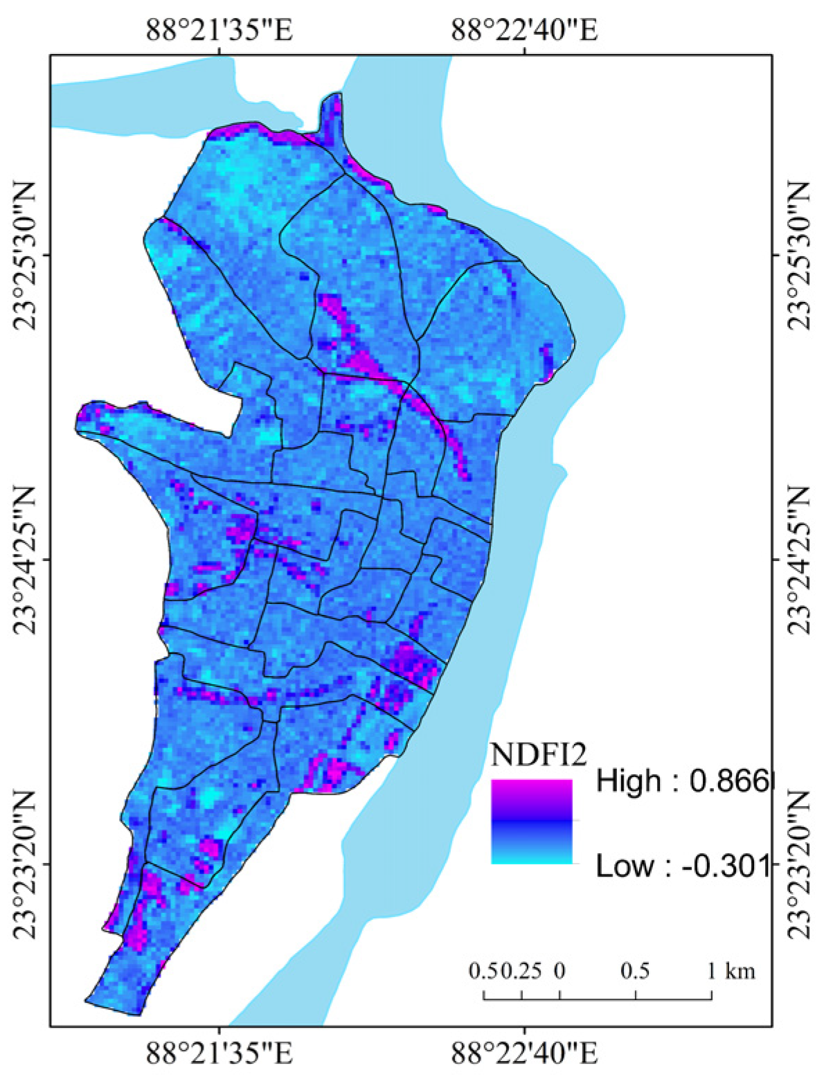
| Normalized Difference Flood Index 3 (NDFI2) | NDFI2 = | [65,66,67] | Satellite imagery-based spectral index of flood conditions. |
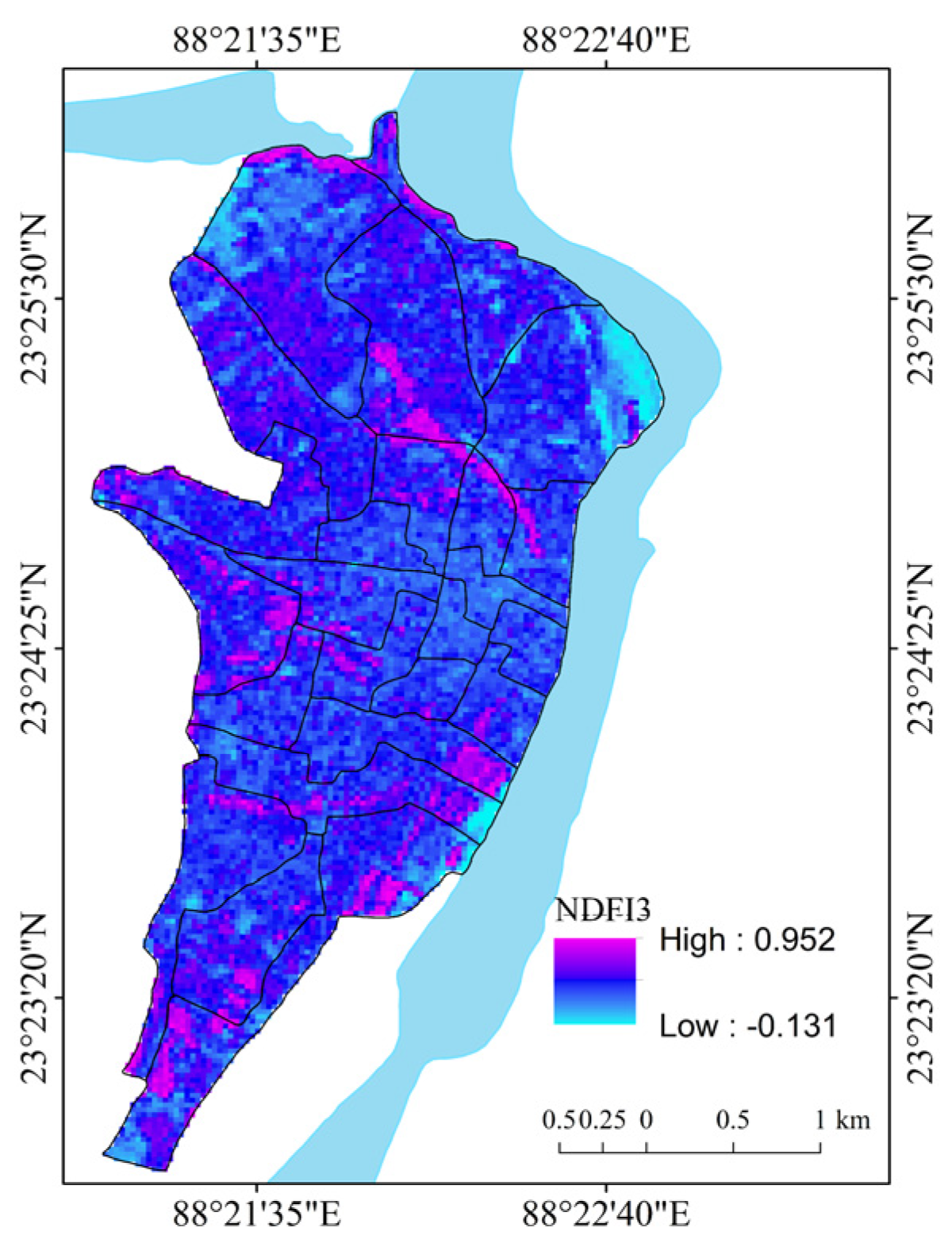
| Normalized Difference Flood Index 3 (NDFI3) | NDFI3 = | [65,67] | Satellite imagery-based spectral index of flood conditions. |
| Year | Month | SPI | Year | Month | SPI | Year | Month | SPI |
|---|---|---|---|---|---|---|---|---|
| 1986 | 1 | −0.48 | 1996 | 1 | −0.70 | 2006 | 1 | 0.33 |
| 1986 | 2 | 0.43 | 1996 | 2 | 0.05 | 2006 | 2 | −1.84 |
| 1986 | 3 | 0.37 | 1996 | 3 | −0.07 | 2006 | 3 | −0.65 |
| 1986 | 4 | −0.58 | 1996 | 4 | −0.15 | 2006 | 4 | 0.00 |
| 1986 | 5 | −0.33 | 1996 | 5 | 0.21 | 2006 | 5 | 0.07 |
| 1986 | 6 | −0.94 | 1996 | 6 | −1.12 | 2006 | 6 | 1.01 |
| 1986 | 7 | 0.57 | 1996 | 7 | 0.07 | 2006 | 7 | 0.86 |
| 1986 | 8 | −0.74 | 1996 | 8 | −0.57 | 2006 | 8 | 1.34 |
| 1986 | 9 | −2.29 | 1996 | 9 | 1.63 | 2006 | 9 | 0.35 |
| 1986 | 10 | 0.44 | 1996 | 10 | −1.46 | 2006 | 10 | 0.37 |
| 1986 | 11 | 0.63 | 1996 | 11 | −0.10 | 2006 | 11 | −0.54 |
| 1986 | 12 | 1.53 | 1996 | 12 | −0.96 | 2006 | 12 | 0.29 |
| 1987 | 1 | 1.05 | 1997 | 1 | −0.53 | 2007 | 1 | −0.44 |
| 1987 | 2 | 0.45 | 1997 | 2 | 1.47 | 2007 | 2 | −1.57 |
| 1987 | 3 | −0.61 | 1997 | 3 | 0.13 | 2007 | 3 | 2.08 |
| 1987 | 4 | −0.33 | 1997 | 4 | 0.77 | 2007 | 4 | −0.23 |
| 1987 | 5 | 0.43 | 1997 | 5 | 0.95 | 2007 | 5 | 0.16 |
| 1987 | 6 | −0.93 | 1997 | 6 | −0.78 | 2007 | 6 | −0.32 |
| 1987 | 7 | −2.45 | 1997 | 7 | −0.07 | 2007 | 7 | −0.55 |
| 1987 | 8 | −1.18 | 1997 | 8 | 1.90 | 2007 | 8 | 2.29 |
| 1987 | 9 | −1.19 | 1997 | 9 | 1.10 | 2007 | 9 | −0.25 |
| 1987 | 10 | −0.98 | 1997 | 10 | −0.91 | 2007 | 10 | 1.27 |
| 1987 | 11 | −1.78 | 1997 | 11 | −2.52 | 2007 | 11 | 0.15 |
| 1987 | 12 | 0.39 | 1997 | 12 | 0.06 | 2007 | 12 | 1.04 |
| 1988 | 1 | 1.05 | 1998 | 1 | 1.82 | 2008 | 1 | −0.35 |
| 1988 | 2 | −1.58 | 1998 | 2 | 1.54 | 2008 | 2 | 1.99 |
| 1988 | 3 | 1.22 | 1998 | 3 | 0.11 | 2008 | 3 | 1.04 |
| 1988 | 4 | −0.02 | 1998 | 4 | 2.25 | 2008 | 4 | −0.24 |
| 1988 | 5 | −0.39 | 1998 | 5 | −0.17 | 2008 | 5 | −0.65 |
| 1988 | 6 | −0.09 | 1998 | 6 | −0.13 | 2008 | 6 | −0.07 |
| 1988 | 7 | 1.10 | 1998 | 7 | 1.47 | 2008 | 7 | 0.56 |
| 1988 | 8 | −1.37 | 1998 | 8 | 0.66 | 2008 | 8 | 0.44 |
| 1988 | 9 | −0.89 | 1998 | 9 | 0.76 | 2008 | 9 | −0.14 |
| 1988 | 10 | −0.59 | 1998 | 10 | 0.49 | 2008 | 10 | 0.48 |
| 1988 | 11 | −1.40 | 1998 | 11 | 0.70 | 2008 | 11 | 0.77 |
| 1988 | 12 | 1.18 | 1998 | 12 | 0.92 | 2008 | 12 | −0.68 |
| 1989 | 1 | 0.06 | 1999 | 1 | −0.32 | 2009 | 1 | −0.22 |
| 1989 | 2 | −1.16 | 1999 | 2 | −1.70 | 2009 | 2 | −0.85 |
| 1989 | 3 | −0.30 | 1999 | 3 | −0.96 | 2009 | 3 | −0.79 |
| 1989 | 4 | 0.07 | 1999 | 4 | −0.42 | 2009 | 4 | −0.11 |
| 1989 | 5 | −0.63 | 1999 | 5 | −1.64 | 2009 | 5 | −0.88 |
| 1989 | 6 | 1.12 | 1999 | 6 | 0.94 | 2009 | 6 | 1.00 |
| 1989 | 7 | −0.20 | 1999 | 7 | −0.26 | 2009 | 7 | −1.64 |
| 1989 | 8 | −0.31 | 1999 | 8 | 1.44 | 2009 | 8 | −0.41 |
| 1989 | 9 | −1.26 | 1999 | 9 | 1.12 | 2009 | 9 | 0.45 |
| 1989 | 10 | −0.11 | 1999 | 10 | 1.53 | 2009 | 10 | 0.18 |
| 1989 | 11 | 0.95 | 1999 | 11 | 0.83 | 2009 | 11 | −0.01 |
| 1989 | 12 | −1.24 | 1999 | 12 | 0.00 | 2009 | 12 | 0.74 |
| 1990 | 1 | 0.88 | 2000 | 1 | −0.27 | 2010 | 1 | −0.36 |
| 1990 | 2 | −0.58 | 2000 | 2 | −0.61 | 2010 | 2 | −0.92 |
| 1990 | 3 | 0.81 | 2000 | 3 | 0.97 | 2010 | 3 | −0.20 |
| 1990 | 4 | 1.61 | 2000 | 4 | −0.24 | 2010 | 4 | −0.22 |
| 1990 | 5 | 0.99 | 2000 | 5 | 0.93 | 2010 | 5 | −0.29 |
| 1990 | 6 | 2.23 | 2000 | 6 | 0.55 | 2010 | 6 | 0.67 |
| 1990 | 7 | −0.27 | 2000 | 7 | −0.01 | 2010 | 7 | −0.62 |
| 1990 | 8 | 0.28 | 2000 | 8 | −0.13 | 2010 | 8 | −0.88 |
| 1990 | 9 | −0.86 | 2000 | 9 | −0.79 | 2010 | 9 | −2.06 |
| 1990 | 10 | −0.54 | 2000 | 10 | 0.49 | 2010 | 10 | −0.27 |
| 1990 | 11 | 1.02 | 2000 | 11 | −0.48 | 2010 | 11 | 0.46 |
| 1990 | 12 | 1.30 | 2000 | 12 | −0.68 | 2010 | 12 | −0.10 |
| 1991 | 1 | 0.45 | 2001 | 1 | −1.47 | 2011 | 1 | 1.28 |
| 1991 | 2 | 1.17 | 2001 | 2 | 0.18 | 2011 | 2 | −0.70 |
| 1991 | 3 | −0.67 | 2001 | 3 | −0.16 | 2011 | 3 | 0.02 |
| 1991 | 4 | −0.13 | 2001 | 4 | 1.51 | 2011 | 4 | 0.48 |
| 1991 | 5 | −1.11 | 2001 | 5 | −0.50 | 2011 | 5 | 0.36 |
| 1991 | 6 | −0.76 | 2001 | 6 | 0.25 | 2011 | 6 | 0.08 |
| 1991 | 7 | 0.05 | 2001 | 7 | 1.45 | 2011 | 7 | 0.73 |
| 1991 | 8 | −0.77 | 2001 | 8 | 0.34 | 2011 | 8 | −0.71 |
| 1991 | 9 | 0.45 | 2001 | 9 | 0.36 | 2011 | 9 | 0.95 |
| 1991 | 10 | 0.16 | 2001 | 10 | −0.75 | 2011 | 10 | 0.02 |
| 1991 | 11 | 0.77 | 2001 | 11 | 1.28 | 2011 | 11 | −1.55 |
| 1991 | 12 | 0.30 | 2001 | 12 | 0.67 | 2011 | 12 | −0.52 |
| 1992 | 1 | 1.66 | 2002 | 1 | −0.41 | 2012 | 1 | −0.26 |
| 1992 | 2 | −0.25 | 2002 | 2 | 1.09 | 2012 | 2 | 1.31 |
| 1992 | 3 | 0.39 | 2002 | 3 | −1.21 | 2012 | 3 | −0.09 |
| 1992 | 4 | −0.22 | 2002 | 4 | 0.07 | 2012 | 4 | −0.66 |
| 1992 | 5 | −0.52 | 2002 | 5 | −0.42 | 2012 | 5 | 0.44 |
| 1992 | 6 | −0.42 | 2002 | 6 | 0.07 | 2012 | 6 | −0.83 |
| 1992 | 7 | −1.07 | 2002 | 7 | 0.22 | 2012 | 7 | −1.58 |
| 1992 | 8 | −0.03 | 2002 | 8 | 0.46 | 2012 | 8 | −0.98 |
| 1992 | 9 | −0.38 | 2002 | 9 | 1.09 | 2012 | 9 | −0.52 |
| 1992 | 10 | −1.07 | 2002 | 10 | 0.50 | 2012 | 10 | 0.95 |
| 1992 | 11 | −1.02 | 2002 | 11 | −0.29 | 2012 | 11 | −0.27 |
| 1992 | 12 | −0.25 | 2002 | 12 | 1.29 | 2012 | 12 | 0.25 |
| 1993 | 1 | −0.45 | 2003 | 1 | −0.56 | 2013 | 1 | 1.20 |
| 1993 | 2 | −0.32 | 2003 | 2 | −0.10 | 2013 | 2 | 0.16 |
| 1993 | 3 | −0.14 | 2003 | 3 | −0.14 | 2013 | 3 | 0.29 |
| 1993 | 4 | 0.67 | 2003 | 4 | 1.28 | 2013 | 4 | −0.84 |
| 1993 | 5 | 1.60 | 2003 | 5 | 1.38 | 2013 | 5 | 0.04 |
| 1993 | 6 | −0.37 | 2003 | 6 | −0.33 | 2013 | 6 | 1.78 |
| 1993 | 7 | 1.16 | 2003 | 7 | 1.29 | 2013 | 7 | 0.96 |
| 1993 | 8 | −0.33 | 2003 | 8 | 0.39 | 2013 | 8 | −0.98 |
| 1993 | 9 | 1.07 | 2003 | 9 | −0.44 | 2013 | 9 | 0.84 |
| 1993 | 10 | 0.66 | 2003 | 10 | −0.59 | 2013 | 10 | 1.17 |
| 1993 | 11 | −0.45 | 2003 | 11 | 1.25 | 2013 | 11 | 0.96 |
| 1993 | 12 | 0.63 | 2003 | 12 | −0.20 | 2013 | 12 | −0.71 |
| 1994 | 1 | −0.88 | 2004 | 1 | 1.65 | 2014 | 1 | −0.33 |
| 1994 | 2 | 0.68 | 2004 | 2 | −0.02 | 2014 | 2 | 0.03 |
| 1994 | 3 | 1.81 | 2004 | 3 | 0.34 | 2014 | 3 | 1.62 |
| 1994 | 4 | 0.12 | 2004 | 4 | −0.08 | 2014 | 4 | 0.16 |
| 1994 | 5 | 0.83 | 2004 | 5 | 1.16 | 2014 | 5 | −1.78 |
| 1994 | 6 | −0.65 | 2004 | 6 | −0.52 | 2014 | 6 | 0.09 |
| 1994 | 7 | 1.03 | 2004 | 7 | 0.41 | 2014 | 7 | −0.91 |
| 1994 | 8 | −0.27 | 2004 | 8 | 0.70 | 2014 | 8 | −0.96 |
| 1994 | 9 | 0.31 | 2004 | 9 | 0.30 | 2014 | 9 | 0.66 |
| 1994 | 10 | −0.89 | 2004 | 10 | 2.53 | 2014 | 10 | −1.20 |
| 1994 | 11 | −0.56 | 2004 | 11 | 0.97 | 2014 | 11 | −0.97 |
| 1994 | 12 | −0.65 | 2004 | 12 | −0.65 | 2014 | 12 | −1.53 |
| 1995 | 1 | 0.00 | 2005 | 1 | −0.17 | 2015 | 1 | 0.59 |
| 1995 | 2 | −0.11 | 2005 | 2 | 0.65 | 2015 | 2 | 1.15 |
| 1995 | 3 | 0.26 | 2005 | 3 | −0.46 | 2015 | 3 | −0.27 |
| 1995 | 4 | −0.45 | 2005 | 4 | 1.49 | 2015 | 4 | 0.37 |
| 1995 | 5 | −1.79 | 2005 | 5 | 1.71 | 2015 | 5 | 1.45 |
| 1995 | 6 | 1.76 | 2005 | 6 | −0.30 | 2015 | 6 | −0.48 |
| 1995 | 7 | 1.02 | 2005 | 7 | −0.91 | 2015 | 7 | −0.80 |
| 1995 | 8 | 0.51 | 2005 | 8 | −0.06 | 2015 | 8 | 1.42 |
| 1995 | 9 | 1.42 | 2005 | 9 | 0.36 | 2015 | 9 | −0.29 |
| 1995 | 10 | 1.08 | 2005 | 10 | −0.26 | 2015 | 10 | −1.02 |
| 1995 | 11 | 0.20 | 2005 | 11 | 2.14 | 2015 | 11 | −0.46 |
| 1995 | 12 | 2.16 | 2005 | 12 | −0.43 | 2015 | 12 | −0.33 |
| Months | Jan | Feb | Mar | Apr | May | Jun | Jul | Aug | Sep | Oct | Nov | Dec |
|---|---|---|---|---|---|---|---|---|---|---|---|---|
| SPI 1-month | ||||||||||||
| 2000 | 1 | 0.05 | −0.46 | 0.94 | −0.29 | 0.75 | 0.55 | 0.04 | −0.26 | −1.17 | −0.64 | −0.49 |
| 2015 | 0.82 | 1.11 | −0.11 | 0.38 | 1.29 | −0.81 | −0.74 | 1.24 | −0.47 | −1.22 | −0.63 | −0.11 |
| SPI 3-month | ||||||||||||
| 2000 | NA | NA | 0.17 | −0.02 | 0.51 | 0.49 | 0.20 | −0.14 | −0.72 | −0.45 | −0.70 | −0.27 |
| 2015 | −1.29 | 0.29 | 0.34 | 0.21 | 0.53 | −0.15 | −0.73 | 0.16 | 0.07 | −0.28 | −1.51 | −1.52 |
| SPI 4-month | ||||||||||||
| 2000 | NA | NA | NA | −0.42 | 0.25 | 0.73 | 0.13 | −0.08 | −0.61 | −0.40 | −0.74 | −0.73 |
| 2015 | −2.20 | −1.13 | −0.09 | 0.12 | 0.78 | −0.54 | −0.71 | 0.28 | −0.09 | −0.57 | −0.59 | −1.52 |
| SPI 6-month | ||||||||||||
| 2000 | NA | NA | NA | NA | NA | 0.41 | 0.13 | −0.08 | −0.59 | −0.30 | −0.58 | −0.67 |
| 2015 | −1.49 | −1.30 | −2.14 | −1.35 | 0.42 | −0.32 | −0.76 | 0.21 | 0.01 | −0.59 | −0.90 | −0.82 |
| SPI 12-month | ||||||||||||
| 2000 | NA | NA | NA | NA | NA | NA | NA | NA | NA | NA | NA | −0.60 |
| 2015 | −1.61 | −1.53 | −1.65 | −1.64 | −1.50 | −1.68 | −1.73 | −0.88 | −1.23 | −0.91 | −0.85 | −0.81 |
| R-Value | ||||||||||||
|---|---|---|---|---|---|---|---|---|---|---|---|---|
| Elevation | Slope | Flow Direction | Flow Distance | Flow Length Line Density | NDVI | NDWI | NDBI | NDSI | NDTI | Distance of Municipal Wards from the Old River Course | Distance of Municipal Wards from the New River Course | |
| Elevation | 1.000 | −0.086 | 0.062 | 0.368 | −0.277 | −0.118 | 0.024 | −0.024 | −0.066 | −0.150 | −0.168 | 0.117 |
| Slope | −0.086 | 1.000 | −0.080 | 0.443 * | 0.018 | 0.058 | −0.092 | 0.092 | 0.015 | 0.017 | 0.502 * | −0.397 |
| Flow Direction | 0.062 | −0.080 | 1.000 | −0.288 | −0.143 | −0.089 | −0.053 | 0.053 | −0.067 | 0.040 | −0.137 | 0.244 |
| Flow Distance | 0.368 | 0.443 * | −0.288 | 1.000 | −0.213 | 0.001 | −0.070 | 0.070 | 0.047 | 0.081 | 0.058 | −0.296 |
| Flow Length Line Density | −0.277 | 0.018 | −0.143 | −0.213 | 1.000 | −0.092 | 0.031 | −0.031 | −0.071 | 0.082 | 0.135 | −0.291 |
| NDVI | −0.118 | 0.058 | −0.089 | 0.001 | −0.092 | 1.000 | 0.676 ** | −0.676 | −0.464* | −0.771 ** | −0.252 | 0.386 |
| NDWI | 0.024 | −0.092 | −0.053 | −0.070 | 0.031 | 0.676 ** | 1.000 | −1.000 | −0.901 ** | −0.718 ** | −0.338 | 0.290 |
| NDBI | −0.024 | 0.092 | 0.053 | 0.070 | −0.031 | −0.676 ** | −1.000 ** | 1.000 | 0.901 ** | 0.718 ** | 0.338 | −0.290 |
| NDSI | −0.066 | 0.015 | −0.067 | 0.047 | −0.071 | −0.464* | −0.901 ** | 0.901 ** | 1.000 | 0.690 ** | 0.246 | −0.134 |
| NDTI | −0.150 | 0.017 | 0.040 | 0.081 | 0.082 | −0.771 ** | −0.718 ** | 0.718 ** | 0.690 ** | 1.000 | 0.234 | −0.327 |
| Distance of municipal wards from the old river course | −0.168 | 0.502* | −0.137 | 0.058 | 0.135 | −0.252 | −0.338 | 0.338 | 0.246 | 0.234 | 1.000 | −0.782 ** |
| Distance of municipal wards from the new river course | 0.117 | −0.397 | 0.244 | −0.296 | −0.291 | 0.386 | 0.290 | −0.290 | −0.134 | −0.327 | −0.782 ** | 1.000 |
 0.3 to 0.7
  >+ −0.7
  . ** Correlation is significant at the 0.01 level (2-tailed). Source: Calculated by the authors.
| R-value | ||||||||||||
|---|---|---|---|---|---|---|---|---|---|---|---|---|
| Elevation | Slope | Flow Direction | Flow Distance | Flow Length Line Density | NDVI | NDWI | NDBI | NDSI | NDTI | Distance of Municipal Wards from the Old River Course | Distance of Municipal Wards from the New River Course | |
| Elevation | 1.000 | −0.634 ** | −0.245 | −0.259 | −0.304 | 0.445 * | 0.040 | 0.406 * | 0.577 ** | 0.445 * | −0.168 | 0.117 |
| Slope | −0.634 ** | 1.000 | 0.405* | 0.604 ** | 0.378 | −0.465 * | 0.006 | −0.380 | −0.466 * | −0.465 * | 0.188 | −0.029 |
| Flow Direction | −0.245 | 0.405 * | 1.000 | 0.101 | −0.058 | −0.099 | 0.224 | −0.185 | 0.132 | −0.099 | −0.106 | 0.234 |
| Flow Distance | −0.259 | 0.604 ** | 0.101 | 1.000 | −0.024 | −0.318 | 0.272 | −0.440 * | −0.106 | −0.318 | 0.165 | −0.083 |
| Flow Length Line Density | −0.304 | 0.378 | −0.058 | −0.024 | 1.000 | −0.512 * | −0.321 | −0.128 | −0.681 ** | −0.512 * | 0.188 | −0.384 |
| NDVI | 0.445 ** | −0.465 * | −0.099 | −0.318 | −0.512* | 1.000 | −0.479 * | 0.841 ** | 0.262 | 1.000 ** | −0.038 | 0.244 |
| NDWI | 0.040 | 0.006 | 0.224 | 0.272 | −0.321 | −0.479 * | 1.000 | −0.792 ** | 0.648 ** | −0.479 * | −0.040 | 0.155 |
| NDBI | 0.406 * | −0.380 | −0.185 | −0.440* | −0.128 | 0.841 ** | −0.792 ** | 1.000 | −0.048 | 0.841 ** | −0.075 | 0.064 |
| NDSI | 0.577 | −0.466* | 0.132 | −0.106 | −0.681 ** | 0.262 | 0.648 ** | −0.048 | 1.000 | 0.262 | −0.155 | 0.329 |
| NDTI | 0.445 * | −0.465 * | −0.099 | −0.318 | −0.512* | 1.000 ** | −0.479 * | 0.841 ** | 0.262 | 1.000 | −0.038 | 0.244 |
| Distance of municipal wards from the old river course | −0.168 | 0.188 | −0.106 | 0.165 | 0.188 | −0.038 | −0.040 | −0.075 | −0.155 | −0.038 | 1.000 | −0.782 ** |
| Distance of municipal wards from the new river course | 0.117 | −0.029 | 0.234 | −0.083 | −0.384 | 0.244 | 0.155 | 0.064 | 0.329 | 0.244 | −0.782 ** | 1.000 |
 0.3 to 0.7
  >+ −0.7
  . ** Correlation is significant at the 0.01 level (2-tailed). Source: Calculated by the authors.
| Variable | Mean | Std. Deviation (Standard Deviation) |
|---|---|---|
| NDFI2 | 0.3396 | 0.08503 |
| Elevation | 16.1529 | 2.64389 |
| Slope | 4.3016 | 2.45902 |
| Flow Direction | 34.4583 | 28.90502 |
| Flow Distance | 1.8811 | 2.01773 |
| Flow Length Line Density | 1.3057 | 0.40098 |
| NDVI | −0.0867 | 0.02213 |
| NDWI | 0.2013 | 0.05387 |
| NDBI | −0.0730 | 0.04289 |
| NDSI | 0.1306 | 0.03364 |
| NDTI | −0.0867 | 0.02213 |
| Distance of municipal wards from the old river course | 1.4396 | 0.72325 |
| Distance of municipal wards from the new river course | 0.9729 | 0.62209 |
| N (total municipal wards) = 24 | ||
| Model Summary b | |||||
|---|---|---|---|---|---|
| Model | R | R Square | Adjusted R Square | Std. Error of the Estimate | Durbin–Watson |
| 0.866 a | 0.750 | 0.557 | 0.05659 | 2.513 | |
| ANOVA a | |||||
|---|---|---|---|---|---|
| Model | Sum of Squares | df | Mean Square | F | Sig. (Significance) |
| Regression | 0.125 | 10 | 0.012 | 3.893 | 0.012 b |
| Residual | 0.042 | 13 | 0.003 | ||
| Total | 0.166 | 23 | |||
| Coefficients a | ||||||||||
|---|---|---|---|---|---|---|---|---|---|---|
| Unstandardized Coefficients | Standardized Coefficients | 95.0% Confidence Interval for B | Collinearity Statistics | |||||||
| Model | B | Std. Error | Beta | t | Sig. | Lower Bound | Upper Bound | Tolerance | VIF (Variance Inflation Factor) | |
| (Constant) | 0.455 | 0.199 | 2.288 | 0.040 | 0.025 | 0.885 | ||||
| Elevation | 0.024 | 0.008 | 0.748 | 2.966 | 0.011 | 0.007 | 0.042 | 0.303 | 3.299 | |
| Slope | 0.017 | 0.013 | 0.485 | 1.265 | 0.228 | −0.012 | 0.045 | 0.131 | 7.624 | |
| Flow Direction | 0.000 | 0.001 | 0.166 | 0.861 | 0.405 | −0.001 | 0.002 | 0.518 | 1.931 | |
| Flow Distance | −0.015 | 0.010 | −0.360 | −1.458 | 0.169 | −0.038 | 0.007 | 0.315 | 3.173 | |
| Flow Length Line Density | 0.054 | 0.060 | 0.254 | 0.900 | 0.384 | −0.076 | 0.183 | 0.241 | 4.145 | |
| NDWI | 4.599 | 1.029 | 2.913 | 4.470 | 0.001 | 2.376 | 6.821 | 0.045 | 22.055 | |
| NDSI | −5.790 | 1.291 | −2.291 | −4.484 | 0.001 | −8.580 | −3.001 | 0.074 | 13.554 | |
| NDTI | 6.476 | 2.267 | 1.685 | 2.857 | 0.013 | 1.579 | 11.373 | 0.055 | 18.067 | |
| Distance of municipal wards from the old river course | −0.106 | 0.046 | −0.903 | −2.304 | 0.038 | −0.206 | −0.007 | 0.125 | 7.971 | |
| Distance of municipal wards from the new river course | −0.093 | 0.057 | −0.677 | −1.634 | 0.126 | −0.215 | 0.030 | 0.112 | 8.920 | |
| a. Dependent Variable: NDFI2 | ||||||||||
| Excluded Variables a | ||||||||||
| Model | Collinearity Statistics | |||||||||
| Beta In | t | Sig. | Partial Correlation | Tolerance | VIF | Minimum Tolerance | ||||
| NDVI | .b | . | . | . | 0.000 | . | 0.000 | |||
| NDBI | 15.410 b | 0.957 | 0.358 | 0.266 | 0.00007472 | 13382.683 | 0.00004458 | |||
| a. Dependent Variable: NDFI2 | ||||||||||
| b. Predictors in the model: (constant), distance of municipal wards from the new river course, slope, NDWI, flow direction, flow length line density, elevation, flow distance, distance of municipal wards from the old river course, NDSI, NDTI | ||||||||||
| R Square (2000) | Elevation | Slope | Flow Direction | Flow Distance | Flow Length Line Density | NDVI | NDWI | NDBI | NDSI | NDTI | Distance of Municipal Wards from the Old River Course | Distance of Municipal Wards from the New River Course |
|---|---|---|---|---|---|---|---|---|---|---|---|---|
| Elevation | 1.000 | 0.007 | 0.004 | 0.135 | 0.077 | 0.014 | 0.001 | 0.001 | 0.004 | 0.023 | 0.028 | 0.014 |
| Slope | 0.007 | 1.000 | 0.006 | 0.196 | 0.000 | 0.003 | 0.008 | 0.008 | 0.000 | 0.000 | 0.252 | 0.158 |
| Flow Direction | 0.004 | 0.006 | 1.000 | 0.083 | 0.020 | 0.008 | 0.003 | 0.003 | 0.004 | 0.002 | 0.019 | 0.060 |
| Flow Distance | 0.135 | 0.196 | 0.083 | 1.000 | 0.045 | 0.000 | 0.005 | 0.005 | 0.002 | 0.007 | 0.003 | 0.088 |
| Flow Length Line Density | 0.077 | 0.000 | 0.020 | 0.045 | 1.000 | 0.008 | 0.001 | 0.001 | 0.005 | 0.007 | 0.018 | 0.085 |
| NDVI | 0.014 | 0.003 | 0.008 | 0.000 | 0.008 | 1.000 | 0.457 | 0.457 | 0.215 | 0.594 | 0.064 | 0.149 |
| NDWI | 0.001 | 0.008 | 0.003 | 0.005 | 0.001 | 0.457 | 1.000 | 1.000 | 0.812 | 0.516 | 0.114 | 0.084 |
| NDBI | 0.001 | 0.008 | 0.003 | 0.005 | 0.001 | 0.457 | 1.000 | 1.000 | 0.812 | 0.516 | 0.114 | 0.084 |
| NDSI | 0.004 | 0.000 | 0.004 | 0.002 | 0.005 | 0.215 | 0.812 | 0.812 | 1.000 | 0.476 | 0.061 | 0.018 |
| NDTI | 0.023 | 0.000 | 0.002 | 0.007 | 0.007 | 0.594 | 0.516 | 0.516 | 0.476 | 1.000 | 0.055 | 0.107 |
| Distance of municipal wards from the old river course | 0.028 | 0.252 | 0.019 | 0.003 | 0.018 | 0.064 | 0.114 | 0.114 | 0.061 | 0.055 | 1.000 | 0.612 |
| Distance of municipal wards from the new river course | 0.014 | 0.158 | 0.060 | 0.088 | 0.085 | 0.149 | 0.084 | 0.084 | 0.018 | 0.107 | 0.612 | 1.000 |
| R square (2015) | Elevation | Slope | Flow Direction | Flow Distance | Flow Length Line Density | NDVI | NDWI | NDBI | NDSI | NDTI | Distance of municipal wards from the old river course | Distance of municipal wards from the new river course |
| Elevation | 1.000 | 0.402 | 0.060 | 0.067 | 0.092 | 0.198 | 0.002 | 0.165 | 0.333 | 0.198 | 0.028 | 0.014 |
| Slope | 0.402 | 1.000 | 0.164 | 0.365 | 0.143 | 0.216 | 0.000 | 0.144 | 0.217 | 0.216 | 0.035 | 0.001 |
| Flow Direction | 0.060 | 0.164 | 1.000 | 0.010 | 0.003 | 0.010 | 0.050 | 0.034 | 0.017 | 0.010 | 0.011 | 0.055 |
| Flow Distance | 0.067 | 0.365 | 0.010 | 1.000 | 0.001 | 0.101 | 0.074 | 0.194 | 0.011 | 0.101 | 0.027 | 0.007 |
| Flow Length Line Density | 0.092 | 0.143 | 0.003 | 0.001 | 1.000 | 0.262 | 0.103 | 0.016 | 0.464 | 0.262 | 0.035 | 0.147 |
| NDVI | 0.198 | 0.216 | 0.010 | 0.101 | 0.262 | 1.000 | 0.229 | 0.707 | 0.069 | 1.000 | 0.001 | 0.060 |
| NDWI | 0.002 | 0.000 | 0.050 | 0.074 | 0.103 | 0.229 | 1.000 | 0.627 | 0.420 | 0.229 | 0.002 | 0.024 |
| NDBI | 0.165 | 0.144 | 0.034 | 0.194 | 0.016 | 0.707 | 0.627 | 1.000 | 0.002 | 0.707 | 0.006 | 0.004 |
| NDSI | 0.333 | 0.217 | 0.017 | 0.011 | 0.464 | 0.069 | 0.420 | 0.002 | 1.000 | 0.069 | 0.024 | 0.108 |
| NDTI | 0.198 | 0.216 | 0.010 | 0.101 | 0.262 | 1.000 | 0.229 | 0.707 | 0.069 | 1.000 | 0.001 | 0.060 |
| Distance of municipal wards from the old river course | 0.028 | 0.035 | 0.011 | 0.027 | 0.035 | 0.001 | 0.002 | 0.006 | 0.024 | 0.001 | 1.000 | 0.612 |
| Distance of municipal wards from the new river course | 0.014 | 0.001 | 0.055 | 0.007 | 0.147 | 0.060 | 0.024 | 0.004 | 0.108 | 0.060 | 0.612 | 1.000 |
| Variable | Criteria Weight (2000) | Criteria Weight (2015) | Presumption of the Relationship with Flood Vulnerability | ||||||||||
|---|---|---|---|---|---|---|---|---|---|---|---|---|---|
| Elevation | 0.11 | 0.21 | - | ||||||||||
| Slope | 0.14 | 0.24 | - | ||||||||||
| Flow Direction | 0.10 | 0.12 | + | ||||||||||
| Flow Distance | 0.13 | 0.16 | - | ||||||||||
| Flow Length Line Density | 0.11 | 0.21 | + | ||||||||||
| NDVI | 0.25 | 0.32 | - | ||||||||||
| NDWI | 0.33 | 0.23 | + | ||||||||||
| NDBI | 0.33 | 0.30 | + | ||||||||||
| NDSI | 0.28 | 0.23 | + | ||||||||||
| NDTI | 0.28 | 0.32 | + | ||||||||||
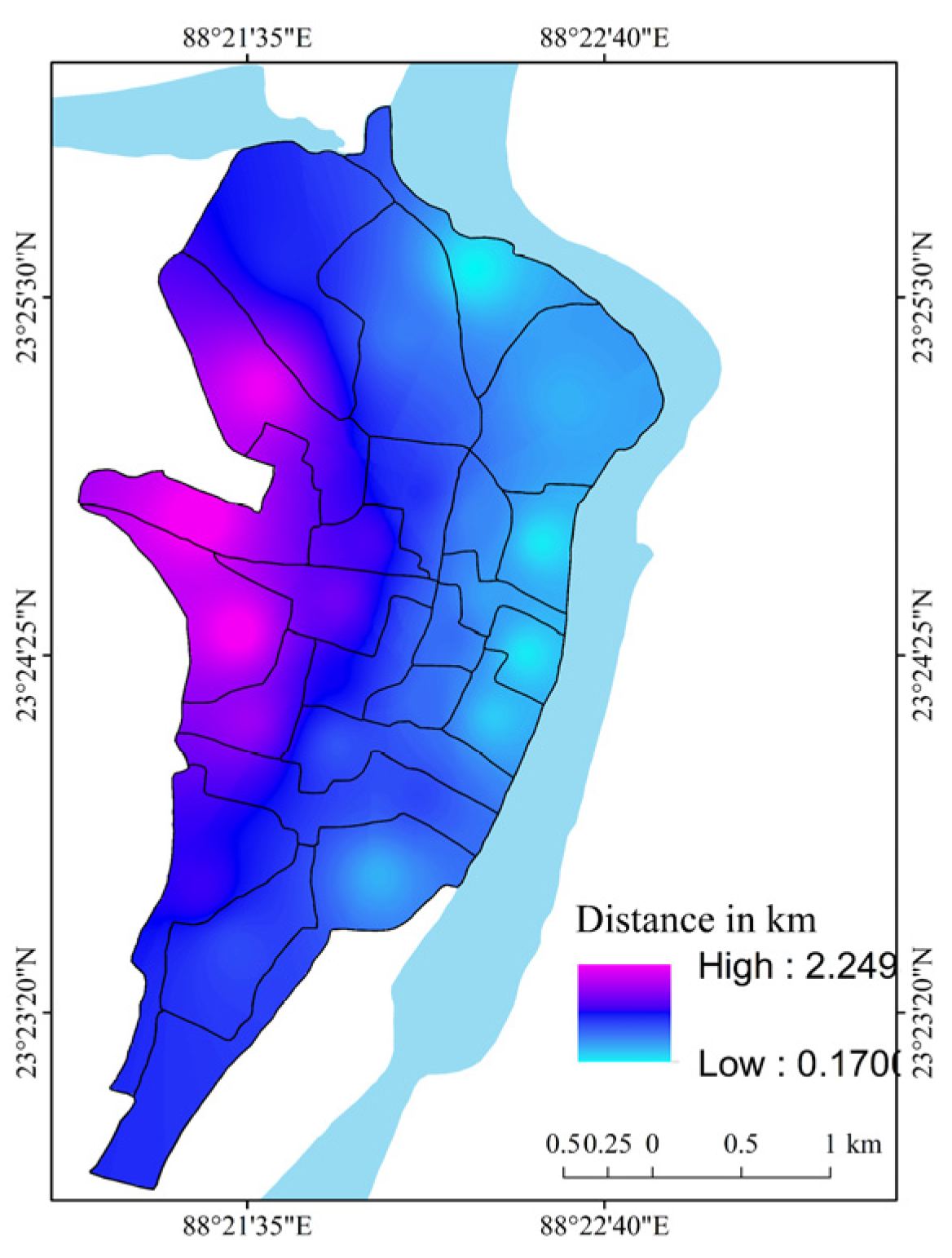
| Distance of municipal wards from the old river course | 0.19 | 0.15 | + | ||||||||||
| Distance of municipal wards from the new river course | 0.20 | 0.17 | - | ||||||||||
| Consistency Index (CI) = 0.156 Consistency Ratio (CR) = 0.101 | Consistency Index (CI) = 0.182 Consistency Ratio (CR) = 0.118 | ||||||||||||
| Source: Calculated by the authors. | |||||||||||||
| Random Index (RI) | |||||||||||||
| n | 1 | 2 | 3 | 4 | 5 | 6 | 7 | 8 | 9 | 10 | 11 | 12 | |
| RI | 0.00 | 0.00 | 0.52 | 0.89 | 1.11 | 1.25 | 1.35 | 1.40 | 1.45 | 1.49 | 1.51 | 1.54 | |
| Ward | Latitude | Longitude | CFVI (2000) | CFVI (2015) | CIb (2015) |
|---|---|---|---|---|---|
| 1 | 23.41379929 | 88.3572998 | 0.086 | 0.292 | 24.00 |
| 2 | 23.41250038 | 88.36569977 | 0.033 | 0.322 | 53.63 |
| 3 | 23.41519928 | 88.36820221 | 0.208 | 0.366 | 34.56 |
| 4 | 23.42040062 | 88.36049652 | 0.204 | 0.386 | 25.51 |
| 5 | 23.42700005 | 88.36199951 | 0.235 | 0.408 | 21.88 |
| 6 | 23.42320061 | 88.36769867 | 0.244 | 0.429 | 27.74 |
| 7 | 23.4197998 | 88.37580109 | 0.253 | 0.451 | 22.90 |
| 8 | 23.41259956 | 88.37460327 | 0.329 | 0.475 | 24.34 |
| 9 | 23.41390038 | 88.37139893 | 0.352 | 0.485 | 36.87 |
| 10 | 23.40990067 | 88.37200165 | 0.991 | 0.491 | 40.27 |
| 11 | 23.40699959 | 88.37380219 | 0.595 | 0.327 | 36.75 |
| 12 | 23.40480042 | 88.36849976 | 0.194 | 0.234 | 41.65 |
| 13 | 23.40800095 | 88.36990356 | 0.358 | 0.239 | 26.85 |
| 14 | 23.40979958 | 88.36419678 | 0.313 | 0.190 | 32.80 |
| 15 | 23.40579987 | 88.3640976 | 0.194 | 0.141 | 36.32 |
| 16 | 23.40810013 | 88.35929871 | 0.063 | 0.123 | 33.25 |
| 17 | 23.40229988 | 88.36440277 | 0.123 | 0.157 | 31.93 |
| 18 | 23.39990044 | 88.36830139 | 0.140 | 0.175 | 31.09 |
| 19 | 23.39579964 | 88.36640167 | 0.096 | 0.193 | 30.25 |
| 20 | 23.39520073 | 88.35739899 | 0.036 | 0.252 | 30.22 |
| 21 | 23.42639923 | 88.37120056 | 0.624 | 0.398 | 25.90 |
| 22 | 23.40390015 | 88.37220001 | 0.157 | 0.080 | 35.08 |
| 23 | 23.40369987 | 88.35970306 | 0.048 | 0.003 | 44.66 |
| 24 | 23.39209938 | 88.35919952 | 0.001 | 0.001 | 24.17 |
| Two-Sample t-Test with Unequal Variances | ||||||
|---|---|---|---|---|---|---|
| Variable | Obs | Mean | Std. Err. | Std. Dev. | 95% Conf. | Interval |
| CFVI (2015) | 24 | 0.27575 | 0.0305024 | 0.1494309 | 0.2126509 | 0.3388491 |
| CIb (2015) | 24 | 32.1925 | 1.576673 | 7.72409 | 28.9309 | 35.4541 |
| combined | 48 | 16.23413 | 2.454992 | 17.00868 | 11.29532 | 21.17293 |
| diff | −31.91675 | 1.576968 | −35.17881 | −28.65469 | ||
| diff = mean (CFVI) − mean (CIb) t = −20.2393 Ho: diff = 0 Welch’s degrees of freedom = 23.0187 | ||||||
| Ha: diff < 0 Ha: diff! = 0 Ha: diff > 0 Pr (T < t) = 0.0000 Pr (|T| > |t|) = 0.0000 Pr (T > t) = 1.0000 | ||||||
| Here, Obs is the number of valid (non-missing) observations used in calculating the t-test, Std. Err. is the standard error, Std. Dev. is the standard deviation, Conf. Interval is the confidence interval, diff denotes difference, Ho = null hypothesis, Ha = alternative hypothesis, and Pr denotes predicted. | ||||||
| SWOC | Code | Relative Importance (Rank) | |
|---|---|---|---|
| Strengths | |||
| 1 | Better road and railway connectivity. | S1 | 1 |
| 2 | A significant number of water bodies. | S2 | 2 |
| Weaknesses | |||
| 1 | Unstructured sewage system. | W1 | 1 |
| 2 | Unplanned built-up areas. | W2 | 4 |
| 3 | Roadways are not properly maintained. | W3 | 3 |
| 4 | Health facilities are inadequate. | W4 | 2 |
| Opportunities | |||
| 1 | Better agricultural production in fringe areas. | O1 | 5 |
| 2 | International importance on tourism. | O2 | 1 |
| 3 | Building up a comprehensive urban development. | O3 | 4 |
| 4 | Participation of local people in flood management. | O4 | 3 |
| 5 | New employment opportunities through the flood management system. | O5 | 2 |
| Challenges | |||
| 1 | River dredging has not been performed. | C1 | 1 |
| 2 | Resettlement is problematic during the flood. | C2 | 4 |
| 3 | Inadequate distribution of flood relief. | C3 | 3 |
| 4 | Indigent damage control network. | C4 | 5 |
| 5 | A large number of poverty-stricken people. | C5 | 2 |
| Matrix | Strengths | Weaknesses | Opportunities | Challenges | ||||||||||||
|---|---|---|---|---|---|---|---|---|---|---|---|---|---|---|---|---|
| S1 | S2 | W1 | W2 | W3 | W4 | O1 | O2 | O3 | O4 | O5 | C1 | C2 | C3 | C4 | C5 | |
| S1 | S1S1 | S1S2 | S1W1 | S1W2 | S1W3 | S1W4 | S1O1 | S1O2 | S1O3 | S1O4 | S1O5 | S1C1 | S1C2 | S1C3 | S1C4 | S1C5 |
| S2 | S2S1 | S2S2 | S2W1 | S2W2 | S2W3 | S2W4 | S2O1 | S2O2 | S2O3 | S2O4 | S2O5 | S2C1 | S2C2 | S2C3 | S2C4 | S2C5 |
| W1 | W1S1 | W1S2 | W1W1 | W1W2 | W1W3 | W1W4 | W1O1 | W1O2 | W1O3 | W1O4 | W1O5 | W1C1 | W1C2 | W1C3 | W1C4 | W1C5 |
| W2 | W2S1 | W2S2 | W2W1 | W2W2 | W2W3 | W2W4 | W2O1 | W2O1 | W2O1 | W2O1 | W2O1 | W2C1 | W2C2 | W2C3 | W2C4 | W2C5 |
| W3 | W3S1 | W3S2 | W3W1 | W3W2 | W3W3 | W3W4 | W2O1 | W2O1 | W2O1 | W2O1 | W2O1 | W3C1 | W3C2 | W3C3 | W3C4 | W3C5 |
| W4 | W4S1 | W4S2 | W4W1 | W4W2 | W4W3 | W4W4 | W4O1 | W4O2 | W4O3 | W4O4 | W4O5 | W4C1 | W4C2 | W4C3 | W4C4 | W4C5 |
| O1 | O1S1 | O1S2 | O1W1 | O1W2 | O1W3 | O1W4 | O1O1 | O1O2 | O1O3 | O1O4 | O1O5 | O1C1 | O1C2 | O1C3 | O1C4 | O1C5 |
| O2 | O2S1 | O2S2 | O2W1 | O2W2 | O2W3 | O2W4 | O2O1 | O2O2 | O2O3 | O2O4 | O2O5 | O2C1 | O2C2 | O2C3 | O2C4 | O2C5 |
| O3 | O3S1 | O3S2 | O3W1 | O3W2 | O3W3 | O3W4 | O3O1 | O3O2 | O3O3 | O3O4 | O3O5 | O3C1 | O3C2 | O3C3 | O3C4 | O3C5 |
| O4 | O4S1 | O4S2 | O4W1 | O4W2 | O4W3 | O4W4 | O4O1 | O4O2 | O4O3 | O4O4 | O4O5 | O4C1 | O4C2 | O4C3 | O4C4 | O4C5 |
| O5 | O5S1 | O5S2 | O5W1 | O5W2 | O5W3 | O5W4 | O5O1 | O5O2 | O5O3 | O5O4 | O5O5 | O5C1 | O5C2 | O5C3 | O5C4 | O5C5 |
| C1 | C1S1 | C1S2 | C1W1 | C1W2 | C1W3 | C1W4 | C1O1 | C1O2 | C1O3 | C1O4 | C1O5 | C1C1 | C1C2 | C1C3 | C1C4 | C1C5 |
| C2 | C2S1 | C2S2 | C2W1 | C2W2 | C2W3 | C2W4 | C2O1 | C2O2 | C2O3 | C2O4 | C2O5 | C2C1 | C2C2 | C2C3 | C2C4 | C2C5 |
| C3 | C3S1 | C3S2 | C3W1 | C3W2 | C3W3 | C3W4 | C3O1 | C3O2 | C3O3 | C3O4 | C3O5 | C3C1 | C3C2 | C3C3 | C3C4 | C3C5 |
| C4 | C4S1 | C4S2 | C4W1 | C4W2 | C4W3 | C4W4 | C4O1 | C4O2 | C4O3 | C4O4 | C4O5 | C4C1 | C4C2 | C4C3 | C4C4 | C4C5 |
| C5 | C5S1 | C5S2 | C5W1 | C5W2 | C5W3 | C5W4 | C5O1 | C5O2 | C5O3 | C5O4 | C5O5 | C5C1 | C5C2 | C5C3 | C5C4 | C5C5 |
Disclaimer/Publisher’s Note: The statements, opinions and data contained in all publications are solely those of the individual author(s) and contributor(s) and not of MDPI and/or the editor(s). MDPI and/or the editor(s) disclaim responsibility for any injury to people or property resulting from any ideas, methods, instructions or products referred to in the content. |
© 2023 by the authors. Licensee MDPI, Basel, Switzerland. This article is an open access article distributed under the terms and conditions of the Creative Commons Attribution (CC BY) license (https://creativecommons.org/licenses/by/4.0/).
Share and Cite
Basu, T.; Mondal, B.K.; Abdelrahman, K.; Fnais, M.S.; Praharaj, S. Assessing Urban Flood Hazard Vulnerability Using Multi-Criteria Decision Making and Geospatial Techniques in Nabadwip Municipality, West Bengal in India. Atmosphere 2023, 14, 669. https://doi.org/10.3390/atmos14040669
Basu T, Mondal BK, Abdelrahman K, Fnais MS, Praharaj S. Assessing Urban Flood Hazard Vulnerability Using Multi-Criteria Decision Making and Geospatial Techniques in Nabadwip Municipality, West Bengal in India. Atmosphere. 2023; 14(4):669. https://doi.org/10.3390/atmos14040669
Chicago/Turabian StyleBasu, Tanmoy, Biraj Kanti Mondal, Kamal Abdelrahman, Mohammed S. Fnais, and Sarbeswar Praharaj. 2023. "Assessing Urban Flood Hazard Vulnerability Using Multi-Criteria Decision Making and Geospatial Techniques in Nabadwip Municipality, West Bengal in India" Atmosphere 14, no. 4: 669. https://doi.org/10.3390/atmos14040669